Journal of Data Science 8(2010), 443-455
An application of Multiple Imputation under the Two Generalized Parametric Families
Hakan Demirtas University of Illinois at Chicago Abstract: Multiple imputation under the multivariate normality assumption has often been regarded as a viable model-based approach in dealing with incomplete continuous data. Considering the fact that real data rarely conform with normality, there has been a growing attention to generalized classes of distributions that cover a broader range of skewness and elongation behavior compared to the normal distribution. In this regard, two recent works have shown that creating imputations under Fleishman’s power polynomials and the generalized lambda distribution may be a promising tool. In this article, essential distributional characteristics of these families are illustrated along with a description of how they can be used to create multiply imputed data sets. Furthermore, an application is presented using a data example from psychiatric research. Multiple imputation under these families that span most of the feasible area in the symmetry-peakedness plane appears to have substantial potential of capturing real missing-data trends that can be encountered in clinical practice. Key words: Kurtosis, multiple imputation, multivariate normality, symmetry, skewness.
1. Introduction and Motivation Missing data are ubiquitous in statistical practice. Determining an appropriate analytical strategy in the absence of complete data presents challenges for scientific exploration. Missing values can give rise to biased parameter estimates, reduced statistical power, and degraded coverage of interval estimates, and thereby may lead to false inferences (Little and Rubin, 2002). Improvements in computational statistics have produced flexible missing-data procedures with a sound statistical basis. One of these procedures involves multiple imputation (MI) (Rubin, 2004), a stochastic simulation technique that replaces each missing datum with a set of plausible values through a predictive distribution. The versions of complete data are then analyzed by standard completedata methods and the results are combined into a single inferential summary using
444
Hakan Demirtas
arithmetic rules to yield estimates, standard errors and p-values that formally incorporate missing data uncertainty into the modeling process. The key ideas and advantages of MI were reviewed by Rubin (1996), Schafer (1997, 1999), and Kenward and Carpenter (2007). For examples of related methods and illustrative applications, see Demirtas and Schafer (2003), Demirtas (2004, 2005), and Demirtas and Hedeker (2007, 2008). The fundamental step in MI is filling in the missing data by drawing from the conditional distribution of the missing data given the observed data which usually entails positing a parametric model for the data and using it to derive this conditional distribution. For continuous data, joint multivariate normality among the variables has often been perceived as a natural assumption since the conditional distribution of the missing data given the observed data is then also multivariate normal. Considering the restrictive nature of the normality assumption, employing a distributional setup that spans a wider range of symmetry-peakedness behavior in the imputation process may provide a reasonable way to handle non-Gaussian continuous data. For this reason, extending the practice of MI from normality to more general classes of densities has begun to receive attention (Liu, 1995; He and Raghunathan, 2006). Demirtas and Hedeker (2008), and Demirtas (2009) demonstrate by simulations that Fleishman’s power polynomials (Fleishman, 1978) and the generalized lambda distribution (GLD) can be thought as sensible alternatives due to their ability of accommodating a variety of distributional shapes depending on the parameter values that can easily be computed for any given data set. Here, we carry out imputation inferences under these flexible methods using a psychiatric clinical trials data in an attempt to explore their performance in a real data context. The organization of the rest of the paper is as follows. In Section 2, I describe salient aspects of Fleishman’s power polynomials. In Section 3, I give an overview of the GLD. Section 4 presents an algorithm for multiply imputing univariate data under these two parametric classes of families. Section 5 includes the real data example, application of the two approaches along with a comparisons to the normal imputation. Concluding remarks, discussion and future directions in the sense of generalizing these methods to the multivariate case are articulated in Section 6. 2. Fleishman Polynomials Fleishman (1978) argued that real-life distributions of variables are typically characterized by their first four moments. He presented a moment-matching procedure that simulates non-normal distributions often used in Monte Carlo studies. It is based on the polynomial transformation, Y = a + bZ + cZ 2 + dZ 3 ,
Imputation under Generalized Families
445
where Z follows a standard normal distribution, and Y is standardized (zero mean and unit variance). The distribution of Y depends on the constants a, b, c and d, whose values were tabulated for selected values of skewness (r1 = E[Y 3 ]) and kurtosis (r2 = E[Y 4 ] − 3). This procedure of expressing any given variable by the sum of linear combinations of powers of a standard normal variate is capable of covering a wide area in the skewness-elongation plane whose bounds are given by the general expression r2 ≥ r12 − 2. 1 High-order moment (the third and fourth moments) boundaries of the power method were given in the original paper (Fleishman, 1978) through an inequality; however, they were not entirely correct. Subsequently, Headrick and Sawilowsky (2000) computed empirical lower bounds of kurtosis for a given value of skewness. Assuming that E[Y ] = 0, and E[Y 2 ] = 1, by utilizing the first 12 moments of the standard normal distribution, the following set of equations can be derived after simple but tedious algebra. Solving these equations can be accomplished by the Newton-Raphson method, or any other plausible root-finding or non-linear optimization routine. a = −c b2 + 6bd + 2c2 + 15d2 − 1 = 0 2c(b2 + 24bd + 105d2 + 2) − r1 = 0 24[bd + c2 (1 + b2 + 28bd) + d2 (12 + 48bd + 141c2 + 225d2 ] − r2 = 0 Fleishman’s method has been extended in several ways in the literature. One extension utilizes the fifth-order polynomials in the spirit of controlling for higherorder moments (Headrick, 2002). The other one is in regard to a multivariate version of the power method. This extension is extremely interesting due to its potential for creating multiply imputed data sets in more realistic multivariate settings (Vale and Maurelli, 1983; Headrick and Sawilowsky, 1999). The generalizability to the multivariate case makes the polynomial method more compelling in the sense that it presents an advantage over other general distributions (Burr family [Burr, 1942], Johnson family [Johnson, 1949], Pearson family [Parrish, 1990], Schmeiser-Deutch system [Schmeiser and Deutch, 1977]) whose multivariate versions are either non-existent or very formidable to specify due to mathematical and/or computational difficulties. The scope of this paper is limited to the univariate case. For this reason, we only briefly mention the operational logic of the multivariate power approach in Section 6 and discuss its connection to the Bayesian multiple imputation technique under the assumption of multivariate normality. A convenience of adapting Fleishman’s method to MI in the 1 It is trivial to prove this by Cauchy-Schwarz inequality. Furthermore, one can show that equality condition is impossible to reach, but this is immaterial for the purposes of this work.
446
Hakan Demirtas
multivariate case is that it allows one to take advantage of well-developed MI methods. In other words, employing suitable transformations makes it possible for practitioners to use existing MI software (e.g. Schimert et al., 2001). It should be noted that the power approach has been criticized by some authors (Tadikamalla, 1980) on the grounds that the exact distribution was unknown and thus lacked probability density and cumulative distribution functions (pdf and cdf, respectively). However, Headrick and Kowalchuk (2007) recently derived the power method’s pdf and cdf in general form. 3. Generalized Lambda Distribution The generalized lambda density is a class of distributions used for parameter estimation, fitting distributions to data, or in simulation studies that primarily involve univariate data generation (Ramberg and Schmeiser, 1972, 1974; Ramberg et al., 1979). The univariate GLD is attractive because its pdf and inverse distribution function are known and its associated algorithm for data generation can be implemented with relative ease. Simulated values, x, can be drawn by the inverse cdf method x = λ1 +[pλ3 −(1−p)λ4 ]/λ2 , where λ1 and λ2 are location and scale parameters, respectively, λ3 and λ4 are shape parameters, and p ∼ U [0, 1]. The right hand side of the equation is the inverse cdf of the GLD. Although the cdf does not exist in closed form, this is not a problem in practice since the same is true for the normal distribution. Estimation of λ’s can be carried out by percentile matching, moment matching, maximum likelihood, and pseudo least squares methods (Tarsitano, 2005). Our preliminary work suggested that matching moments yield very accurate estimates of λ’s. For this reason, we predicate the estimation process upon moment matching. Ramberg and Schmeiser (1974) showed that the k th moment of the GLD, when it exists, is given by
k
E(X ) =
λ−k 2
k ( ) ∑ k i=0
i
(−1)i B(λ3 (k − i) + 1, λ4 i + 1)
for λ1 = 0, where B denotes the beta function. Ramberg et al. (1979) gave details of estimation and model-fitting procedures for this four-parameter probability distribution. It involves solving a set of equations that are formed through the first four moments that are capable of accommodating a wide variety of curve shapes. Ramberg and Schmeiser (1974) derived the following expression for the mean (µ), the variance (σ 2 ), and the third (µ3 = E(X − µ)3 ) and fourth (µ4 = E(X − µ)4 ) moments about the mean for this distribution:
Imputation under Generalized Families
447
A λ2 (B − A2 ) λ22 (C − 3AB + 2A3 ) λ32 (D − 4AC + 6A2 B − 3A4 ) , λ42
µ = λ1 + σ2 = µ3 = µ4 = where A = B = C = D =
1 1 − 1 + λ3 1 + λ4 1 1 + − 2β(1 + λ3 , 1 + λ4 ) 1 + 2λ3 1 + 2λ4 1 1 − − 3β(1 + 2λ3 , 1 + λ4 ) + 3β(1 + λ3 , 1 + 2λ4 ) 1 + 3λ3 1 + 3λ4 1 1 + − 4β(1 + 3λ3 , 1 + λ4 ) 1 + 4λ3 1 + 4λ4 − 4β(1 + λ3 , 1 + 3λ4 ) + 6β(1 + 2λ3 , 1 + 2λ4 ).
The skewness and kurtosis, as given by α3 = σµ33 and α4 = σµ44 − 3 are functions of λ3 and λ4 , but do not depend on λ1 and λ2 . One can easily compute the empirical moments µ∗ , σ ∗2 , µ∗3 , and µ∗4 from a given data set; then find the values of λ3 and λ4 which best solve the two simultaneous nonlinear equations α3 (λ3 , λ4 ) = α3∗ and α4 (λ3 , λ4 ) = α4∗ . As in Fleishman’s method, one can solve these equations by the Newton-Raphson method, or any other plausible root-finding or non-linear optimization routine. Calculating λ1 and λ2 is straightforward, with a caveat that the sign of λ2 should be the same as the sign of λ3 and λ4 . The specification of any feasible moment structure that translates to corresponding values of λ’s, enables us to generate random numbers via the inverse cdf method, which is equally applicable in the context of creating multiply imputed data sets. 4. Imputation Algorithm After reviewing the highlights of the power method and the GLD, I now describe how one utilizes these families in creating multiply imputed data sets. We assume three imputation models for comparison purposes. The first one is the normal model, where we create imputations following the standard approach of using a Bayesian predictive model of the missing data given the observed data
448
Hakan Demirtas
(Schafer, 1997). For the power polynomials, instead of adopting a Bayesian approach, we account for the parameter uncertainty by obtaining nonparametric bootstrap samples that anchor the subsequent estimation procedure for the parameters of the power expression, as was done by He and Raghunathan (2006). Denoting the data Y = (Yobs , Ymis ) = (y1 , y2 , ..., yn1 , yn1 +1 , ..., yn )T , of which the first n1 elements are observed (Yobs = (y1 , y2 , ..., yn1 )T ), and the remaining n − n1 elements are missing (Ymis = yn1 +1 , ..., yn )T ), the imputation algorithm is as follows: 1. Center and scale the data so that mean is zero and variance is one. This standardization is needed for the subsequent estimation of the four power ∗ . polynomial coefficients. Let the transformed data be Yobs ∗ . 2. Draw a nonparametric bootstrap sample of size n1 from Yobs
3. Estimate the model parameters (a, b, c, d) using the Newton-Raphson algorithm.2 4. Simulate independent variates from these distributions for every missing ∗ . data point in Ymis 5. Back transform the filled-in data and the transformed observed data to the original scale. 6. Repeat steps 2-5 independently m = 10 times. For the GLD, the above steps are the same except for Step 3, where the parameters under consideration are (λ1 , λ2 , λ3 , λ4 ) rather than (a, b, c, d). 5. Application Our real data example comes from a study in psychiatric research (Reisby et al., 1977). It was fairly extensively discussed in Hedeker and Gibbons (2006). This study focused on the longitudinal relationships between imipramine (IMI) and desipramine (DMI) plasma levels and clinical response in 66 depressed inpatients. Imipramine is the prototypic drug in the series of compounds known as tricyclic antidepressants, and is commonly prescribed for the treatment of major depression. The study design was as follows. Following a placebo period of one week, patients received 225 mg/day doses of imipramine for four weeks. In this study, 2 There is nothing magical about the Newton-Raphson method, one can use any other plausible root-finding algorithm.
449
10
-20
-15
-10
-5
0
5
10
-20
-10
0
10
-20
-10
0
10
-30
-20
-10
HDRS3
0
10
HDRS4
0
50
100
150
200
250
25 20 15
15 0
100
200
300
10 0
50
100
IMI2
150
200
250
300
0
50
100
IMI3
150
200
250
IMI4
3
4
2
3
4
5
15 10 3
400
500
600
5
6
2
3
4
5
LIMI4
20 0
5
5
10
10
15
15
20
20 15 10 5 0 300
4
25
25
40 30
200
2
LIMI3
20 10
100
0
6
LIMI2
0 0
5
10 5
5
LIMI1
0
200
400
600
800
0
200
DMI2
400
600
800
0
100
200
300
DMI3
400
500
600
DMI4
0
2
4 LDMI1
6
20
15 10
15 10
5
5 3
4
5 LDMI2
6
7
0
0
0
0
5
5
10
10
15
20
15
25
20
30
20
DMI1
0
2
0
0
0
5
5
10
10
15
15
15
20
IMI1
0
5
5 0
0
0
5
10
10
10
15
20
20
20
25
30
25
30
HDRS2
30
HDRS1
0
0
0
0
2
5
5
5
4
10
6
10
15
8
10
15
15
20
25
20
14
20
30
Imputation under Generalized Families
3
4
5 LDMI3
6
7
3
4
5
6
LDMI4
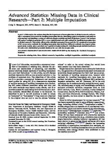
Figure 1: Histogram of HDRS, IMI, LIMI, DMI, and LDMI rows 1, 2, 3, 4, and 5, respectively. The numbers represent the time points (columns 1 through 4 stand for weeks 1 to 4, in that order).
subjects were rated with the Hamilton Depression Rating Scale (HDRS) [Hamilton, 1960] twice during the baseline placebo week (at the start and end of this week) as well as the end of each of the four treatment weeks of the study. These HDRS scores represent the outcome variable that is measured across time. Higher scores on the HDRS represent higher levels of depression and lower scores indicate less depression. Plasma level measurements of both IMI and its metabolite DMI were made at the end of each week. The sex and age of each patient was recorded and a diagnosis of endogenous and nonendogenous depression was made for each patient. Although the total number of subjects in this study was 66, the number of subjects with all measures at each of the week fluctuated, ranging from 58 to 65. Of the 66 subjects, only 46 had complete data at all time points. For the purpose of this work, we focus on change in HDRS since the baseline, IMI and DMI measurements for the four drug weeks. In what follows, HDRS stands for the difference of HDRS with respect to the baseline measurement across four weeks. Previous analyses (Hedeker and Gibbons, 2006) treated HDRS as the outcome, and IMI and DMI as time-varying covariates. In addition, for illustration of the imputation techniques presented in this paper, we add a hypothetical group of
450
Hakan Demirtas
34 subjects whose have no measurements for any of these three variables under consideration, making the total sample size 100. After this adjustment, nonresponse rate is about 40% which is fairly typical in such studies. This situation is not uncommon in clinical practice; it is natural to lose subjects between recruitment time and the start of the treatment. The implied missingness mechanism is missing completely at random (MCAR), in the sense of Rubin (1976). This assumption is unrealistically simplistic in practice, but the scope of this paper is limited to univariate imputation, and more realistic mechanisms are not feasible to formulate in a univariate setting. Table 1: Comparison of the quantiles of observed data and imputed portion across 10 imputations under the normal, Fleishman, and GLD models for HDRS across four time points. Ranks of absolute deviations from the truth are given in brackets, with 1 and 3 corresponding to the least and most biased estimates, respectively. Variable
HDRS1
HDRS2
HDRS3
HDRS4
Quantile
Original data
Normal
Fleishman
GLD
5th 25th 50th 75th 95th 5th 25th 50th 75th 95th 5th 25th 50th 75th 95th 5th 25th 50th 75th 95th
-13.85 -8.25 -4.00 -2.00 2.00 -20.60 -10.00 -6.00 -3.00 3.60 -21.90 -13.00 -10.00 -5.00 2.00 -23.00 -16.00 -11.00 -6.00 0.45
-13.39[2] -8.84[3] -5.07[2] -1.25[2] 3.66[3] -16.73[3] -11.83[3] -7.46[3] -3.06[1] 3.31[1] -21.40[1] -14.37[1] -9.16[3] -4.40[2] 2.67[3] -23.35[1] -16.66[3] -11.75[3] -6.98[3] 0.15[2]
-14.01[1] -8.58[2] -4.77[1] -1.16[3] 3.09[1] -17.47[2] -10.86[2] -6.56[2] -2.92[2] 3.28[2] -20.95[2] -15.32[3] -10.46[2] -4.63[1] 1.87[1] -22.33[2] -16.16[1] -11.40[2] -6.21[2] 0.83[3]
-13.21[3] -8.43[1] -5.08[3] -1.71[1] 3.12[2] -17.82[1] -10.76[1] -6.26[1] -2.88[3] 3.98[3] -20.35[3] -15.23[2] -10.44[1] -5.64[3] 1.76[2] -22.06[3] -16.29[2] -11.37[1] -5.95[1] 0.73[1]
Since IMI and DMI are positively skewed, I also examined logarithmically transformed versions, LIMI and LDMI, where LIM I = log(IM I + 1), and LDM I = log(DM I + 1) (1 was added to accommodate 0 values). Histograms of HDRS, IMI, LIMI, LIMI, and LDMI for four time points are shown in Figure 1 (the numbers at the end of each variable denote the time points). The normal, Fleishman, and GLD imputation models were applied to these five variables at four time points separately. 10 imputations were created for each of these 20 combinations. Admittedly, performing MI separately for 5 × 4 = 20 times is rather peculiar. Again, the reason for this is that the proposed
Imputation under Generalized Families
451
methods have been developed for univariate data. For a discussion of multivariate augmentations, see Section 6. The parameters of interest were chosen to be the five quantiles (5th , 25th , 50th , 75th , and 95th ) that are known to be sensitive to model misspecification. Tables 1 tabulates the five quantiles for the original HDRS data, and averaged quantiles of the imputed portions across 10 multiply imputed data sets for the normal, Fleishman and GLD imputation models. Under MCAR, observed data and imputed values should have similar distributional properties. Ranks based on absolute deviations from the observed data quantiles are shown in brackets, with 1 and 3 corresponding to the least and most biased estimates, respectively. The results for IMI, LIMI, DMI and LDMI are not reported due to space limitations. Full results are accessible at http : //tigger.uic.edu/ ∼ demirtas/tablesJDS.pdf . Examining Table 1 and tables posted on the above-mentioned website clearly reveals the superior performance of the Fleishman and GLD imputation over the normal imputation. The performance differences are most substantial for IMI and DMI for which departures from normality are the most severe. Even for HDRS and log-transformed versions (LIMI and LDMI), where the normality assumption is a close approximation to reality, the comparative performance of the power and GLD approaches is better, although the differences are not very dramatic. In order to make the results more compact and visible, average ranks for HDRS, IMI, LIMI, DMI, and LDMI aggregated across four time points, and overall rank were computed as shown in Table 2. Both Fleishman and GLD imputation models lead to less biased estimates compared to the normal imputation model, in varying degrees depending on the underlying distributional features. Of note, no significant differences were detected between the two general families. Table 2: Average ranks for HDRS, IMI, LIMI, DMI, and LDMI aggregated across four time points, and overall rank. Variable HDRS IMI LIMI DMI LDMI OVERALL
Normal
Fleishman
GLD
2.25 2.65 2.20 2.65 2.05 2.36
1.85 1.65 1.90 1.60 1.95 1.79
1.90 1.70 1.90 1.75 2.00 1.85
6. Discussion In this paper we have implemented methods that were developed in the random number generation literature to the context of MI. A major imputation
452
Hakan Demirtas
principle is not to distort the marginal distributions and associations between observed and imputed variables; and random number generation is conducted via specified distributional properties. Observed data trends can be assumed to be applicable to the whole data set, and missing portions can be filled in with numbers that belong to the same distributional mechanism which, in a sense, is the operational logic for random number generation. This assertion clearly assumes ignorable nonresponse (once we have taken into account what we have observed, there remains no dependence on what we have not observed), where missingness fully depends on the observed quantities in the system in the sense of Rubin (1976). Although this may be considered a limitation, it might serve as a milestone for nonignorable extensions. The promising results in the univariate case substantiate the natural continuation of these imputation methods under the multivariate case. As articulated in Vale and Maurelli (1983), one can compute estimated power coefficients marginally for each variable and correlations among them. Then, by a principle components factorization or another factorization method, an identity that involves powers of the correlation between pairs of standard normal variables and between pairs of the original variables could be obtained. Solving this third-order equation for each pair of standard normal variables, along with marginal coefficients, yields the set of parameters of a multivariate normal distribution. After the generation of the multivariate normal data matrix, it is back-transformed to the original scale. While this approach was suggested in the context of random number generation, it can easily be implemented for incomplete data problems in the following way. After computing the marginal coefficients and correlations for the observed part of the data, a conversion to the multivariate normal case can be done in a straightforward way. Subsequently, one may resort to well-developed Bayesian imputation techniques (Schafer, 1997) under the normal model. Once multiply imputed data sets are created, a back transformation would result in completed data sets that preserve the original features of the data. In a similar spirit, in terms of multivariate data generation, it has been demonstrated by Headrick and Mugdadi (2006) that the GLD have computational difficulties associated with 1) having to take several steps to overcome the problem of generating biased correlation coefficients, 2) having access to commercial software packages and ensuring the accuracy of numerical solutions to complicated integrals. Headrick and Mugdadi (2006) developed a methodology to simulate multivariate non-normal distributions from the GLD. Making connections from random generation domain to MI domain using a multivariate version of the GLD is an exciting idea which will be taken up in future work. There are a few limitations that need to be addressed. First, while we recognize that real incomplete data often include many variables, our focus was on
Imputation under Generalized Families
453
univariate data. We view this as a potential building block for more realistic situations. The behavior of the third and fourth moments typically requires more modeling flexibility in terms of the area covered in the symmetry-elongation plane as well as the association among variables. On a related note, although the power and GLD approaches are capable of picking some data trends that are unlikely to be captured by a normal model, these parametric families do not cover the entire symmetry-elongation plane. Nevertheless, considering the relative gains presented in this paper, it provides an indication that the multivariate version can lead to further improvements. Furthermore, the implied missingness mechanism is generally too simplistic for real-life applications. However, our purpose was not to conduct a sensitivity analysis with respect to the mechanism that leads to the observed data. Rather, the current paper was motivated by how tenably MI inferences can be conducted with power polynomials and the GLD. References Burr, I. W. (1942). Cumulative frequency functions. Annals of Mathematical Statistics 13, 215-232. Demirtas, H. (2004). Simulation-driven inferences for multiply imputed longitudinal datasets. Statistica Neerlandica 58, 466-482. Demirtas, H. (2005). Multiple imputation under Bayesianly smoothed pattern-mixture models for non-ignorable drop-out. Statistics in Medicine 24, 2345-2363. Demirtas, H. (2009). Imputation under the generalized lambda distribution. Journal of Biopharmaceutical Statistics, 19, (in press). Demirtas, H. and Hedeker, D. (2007). Gaussianization-based quasi-imputation and expansion strategies for incomplete correlated binary responses. Statistics in Medicine 26, 782-799. Demirtas, H. and Hedeker, D. (2008). Multiple imputation under power polynomials. Communications in Statistics- Simulation and Computation 37, 1682-1695. Demirtas, H. and Schafer, J. L. (2003). On the performance of random-coefficient pattern-mixture models for non-ignorable drop-out. Statistics in Medicine 22, 2553-2575. Fleishman, A. I. (1978). A method for simulating non-normal distributions. Psychometrika 43, 521-532. Hamilton, M. (1960). A rating scale for depression. Journal of Neurology and Neurosurgical Psychiatry 23, 56-62. He, Y. and Raghunathan, T. E. (2006). Tukey’s gh distribution for multiple imputation. The American Statistician 60, 251-256.
454
Hakan Demirtas
Headrick, T. C. (2002). Fast fifth-order polynomial transforms for generating univariate and multivariate nonnormal distributions. Computational Statistics and Data Analysis 40, 685-711. Headrick, T. C. and Kowalchuk, R. K. (2007). The power method transformation: its probability density function, distribution function, and its further use for fitting data. Journal of Statistical Computation and Simulation 77, 229-249. Headrick, T. C. and Mugdadi, A. (2006). On simulating multivariate non-normal distributions from the generalized lambda distribution. Computational Statistics and Data Analysis, 50, 3343-3353. Headrick, T. C. and Sawilowsky, S. S. (1999). Simulating correlated multivariate nonnormal distributions. Psychometrika 64, 25-35. Headrick, T. C. and Sawilowsky, S. S. (2000). Weighted simplex procedures for determining boundary points and constants for the univariate and multivariate power methods. Journal of Educational and Behavioral Statistics 25, 417-436. Hedeker, D. and Gibbons, R. D. (2006). Longitudinal Data Analysis. John Wiley. Johnson, N. L. (1949). Systems of frequency curves generated by methods of translation. Biometrika 36, 149-176. Kenward, M. G. and Carpenter, J. (2007). Multiple imputation: current perspectives. Statistical Methods in Medical Research 16, 199-218. Little, R. J. A. and Rubin D. B. (2002). Statistical Analysis with Missing Data. Wiley. Liu, C. (1995). Missing data imputation using the multivariate t distribution. Journal of Multivariate Analysis 53, 139-158. Parrish, R. S. (1990). Generating random deviates from multivariate Pearson distributions. Computational Statistics and Data Analysis 9, 283-295. Ramberg, J. S. and Schmeiser, B. W. (1972). An approximate method for generating symmetric random variables. Communications of the ACM 15, 987-990. Ramberg, J. S. and Schmeiser, B. W. (1974). An approximate method for generating asymmetric random variables. Communications of the ACM 17, 78-82. Ramberg, J. S. et al. (1979). A probability distribution and its uses in fitting data. Technometrics 21, 201-214. Reisby, N. et al. (1977). Imipramine: clinical effects and pharmacokinetic variability. Psychopharmacology 54, 263-272. Rubin, D. B. (1976). Inference and missing data. Biometrika 63, 581-592. Rubin, D. B. (1996). Multiple imputation after 18+ years (with discussion). Journal of the American Statistical Association 91, 473-520. Rubin, D. B. (2004). Multiple Imputation for Nonresponse in Surveys. Wiley Classic Library.
Imputation under Generalized Families
455
Schafer, J. L. (1997). Analysis of Incomplete Multivariate Data. Chapman and Hall. Schafer, J. L. (1999). Multiple imputation: a primer. Statistical Methods in Medical Research 8, 3-15. Schimert, J. et al. (2001). Analyzing Data with Missing Values in S-plus. Data Analysis Products Division, Insightful Corp. , Seattle, WA. Schmeiser, B. W. and Deutch, S. J. (1977). A versatile four parameter family of probability distributions suitable for simulation. IIE Transactions 9, 176-182. Tadikamalla, P. R. (1980). On simulating non-normal distributions. Psychometrika 45, 273-279. Tarsitano, A. (2005). Estimation of the generalized lambda distribution parameters for grouped data. Communications in Statistics-Theory and Methods 34, 1689-1709. Vale, C. D. and Maurelli, V. A. (1983). Simulating multivariate nonnormal distributions. Psychometrika 48, 465-471. Received July 14, 2008; accepted December 12, 2008.
Hakan Demirtas Division of Epidemiology and Biostatistics University of Illinois at Chicago, 1603 West Taylor Street, Room 950 Chicago, IL, USA
[email protected]