An Approximation Algorithm for the Subpath Planning Problem - IJCAI

Proceedings of the Twenty-Fifth International Joint Conference on Artificial Intelligence (IJCAI-16)

An Approximation Algorithm for the Subpath Planning Problem Masoud Safilian† , S. Mehdi Hashemi† , Sepehr Eghbali†⇤ , Aliakbar Safilian‡ † Amirkabir University of Technology, Tehran, Iran †⇤ University of Waterloo, Ontario, Canada ‡ McMaster University, Ontario, Canada {m.safilian, hashemi}@aut.ac.ir, [email protected], [email protected] Abstract The subpath planning problem (SPP) is a branch of path planning problem, which has widespread applications in automated manufacturing process as well as vehicle and robot navigation. This problem aims to find the shortest path or tour subject to covering a set of given subpaths. By casting SPP to a graph routing problem, we propose a deterministic 2-approximation algorithm finding near optimal solutions, which runs in O(n3 ) time.

1

Introduction

The path planning problem is a fundamental problem in artificial intelligence and robotics with applications also in other areas such as computer animation and computer games. Due to its applications, several variants of this problem, including planning subject to spatial constraints, have been proposed over the past few years [Nash et al., 2009; Kapadia et al., 2013; Jaillet and Porta, 2013; Surynek, 2015]. In this paper, we focus on Subpath Planning Problem (SPP), which is a constraint path planning problem. Given a set of subpaths, the goal of SPP is to find the shortest tour that travels all given subpaths. SPP is an NP-hard problem with widespread applications. For example, in polishing robot [Tong-ying et al., 2004] the target is to polish nicks on a surface of a workpiece. Nicks, which can be considered as the subpaths, are often extracted by using image processing techniques and the goal is to polish all nicks with minimum arm movement. Also, SPP has applications in electronic printing [Gyorfi et al., 2010], where the continuous-spray processes are used to deposit electrically functional material onto flexible substrate. Moreover, SPP can be used in search and rescue operations as well as aerial image using UAV, where the robot must traverse some specific paths. Fig. 1.a and Fig. 1.b show a toy example of SPP workspace and its optimal solution, respectively. A formal definition of SPP can be found in [Gyorfi et al., 2010]. However, not much attention has been paid to solving this special widely used problem. Only a few approaches have been proposed, which are all meta-heuristic based. For instance, in [Tong-ying et al., 2004] and [Gyorfi et al., 2010] two algorithms based on Genetic Algorithm (GA) [Goldberg, 1989] are proposed for solving SPP in polishing robots and

Figure 1: a) A toy example of SPP workspace (subpaths are shown in dashed lines), b) The optimal solution for the given workspace, c) Graph G, d) Graph G0 . electronic printing, respectively. The major deficiency of such techniques is that, they cannot guarantee any bound on their final output due to their meta-heuristic (and random) nature. More importantly, GA needs considerable amount of time in order to converge to a sub optimal solution, especially for large-scale problems. In its graph theoretical abstraction, SPP is a graph routing problem with close connections to the Travelling Salesman with Neighbours (TSPN) [Papadimitriou, 1977; Safra and Schwartz, 2006], Rural Postman Problem (RPP) [Eiselt et al., 1995b; Orloff, 1974], and Stacker Crane Problem (SCP) [Coja-Oghlan et al., 2006; Frederickson, 1979]. However, SPP is different from these graphical problems in some aspects, which makes their solutions not applicable to the SPP. The present paper addresses the deficiencies of metaheuristic methods for solving SPP by proposing an approximation algorithm with a constant approximation bound and efficient polynomial time complexity. As the first step, given n subpaths, we transform the SPP to the general Travelling Salesman Problem (TSP). By transforming SPP to TSP, it may seem easy to apply the existing constant-factor approximation algorithms of TSP for solving SPP. However, this is not feasible, as the edge weights in the graph of SPP are not metric, i.e., they do not necessarily sat-

669

isfy the triangle inequality. To mitigate this problem, in the second step, we propose an algorithm, called Imperfectly Establish the Triangle Inequality (IETI), which establishes the triangle inequality for a large subset of violating triangles (the triangles that violates the triangle inequality in the graph of SPP). We show that solving SPP on the original graph would be equivalent to solving TSP on the modified graph. The IETI algorithm runs in O(n2 ) time and is a fundamental step for designing an algorithm with a constant approximation factor for solving SPP. Nonetheless, a subset of triangles may still violate the triangle inequality in the graph returned by IETI algorithm. To tackle this problem, in the third step, we propose a 2approximation algorithm, called Christofides for SPP (CSPP) that is in a O(n3 ) time complexity. The CSPP bears some similarities to Christofides algorithm [Christofides, 1976] and is adapted to work for all outputs of the IETI algorithm. Christofides algorithm is a well-known 1.5-approximation algorithm for solving TSP due to its small approximation factor and polynomial time complexity (O(n3 )). In addition to complexity analysis and proving the approximation bound of CSPP, we empirically compare it with the method proposed in [Gyorfi et al., 2010] over various workspaces with different numbers of subpaths. The results indicate that CSPP is more efficient than the other existing methods both in terms of cost of the solution and running time. The rest of the paper is organized as follows: Sections 2, 3, and 4 discuss the transformation, IETI, and CSPP algorithms, respectively. Section 5, presents the experimental results and analysis. Section 6 concludes the paper and presents some potential future directions. Due to the space limitation, some details including the full proofs of the theorems are not described in the paper. We refer the interested reader to the accompanying techinical report [Safilian et al., 2016] for more details.

2

workspace. Let us call this edge the i-th subpath edge. 3. For each pair of subpaths such as i and j (i 6= j), we add edges si ej , ei sj , si sj and ei ej to the graph. We also consider the weights of these newly added edges equal to the corresponding Euclidean distances in the workspace. Let us call these edges the connecting edges. The TSP tour of G is not necessarily a solution for the given SPP instance, since the TSP tour of G may not cover all subpath edges (such as si ei ). To make sure that the TSP tour would travel all subpaths, a complete graph, denoted by G0 , is constructed based on G as follows: 4. For each i-th subpath, a node mi is added to the graph, called the middle node of i-th subpath. 5. For each i-th subpath, two edges si mi and mi ei are added to the graph, the weights of which are equal to the half of the subpath length. These edges are called i-th double subpath edges. 6. For each middle node mi , the edge mi v, where v 2 / {si , ei }, is added to the graph with infinite weight.

Fig. 1.c and Fig. 1.d show the graphs G and G0 for a problem with 4 subpaths, respectively. Theorem 1 A solution of SPP on a given instance corresponds to a solution of TSP in G0 . Proof: It is clear that there is a finite Hamiltonian tour in G0 (see Fig. 1.d). The TSP tour over G0 is a Hamiltonian tour with the minimum weight. Therefore, the TSP tour over G0 is finite. The TSP tour of G0 visits all the middle nodes since for each i, it contains two edges crossing the node mi . There are only two finite edges, namely si mi and mi ei , connected to mi . Hence, the TSP tour over G0 must contain si mi and mi ei for each i. Since si mi and mi ei together are equivalent to the i-th subpath in the workspace, the TSP tour of G0 is the minimum weight which travels all subpaths. We can conclude that solving SPP is equivalent to finding the TSP tour in G0 . It is easy to show that the cost of constructing graph G and G0 is O(n2 ). ⇤

Transformation of SPP to TSP

The solutions of an SPP problem are the tours that travel all subpaths and an optimal solution is a tour with the minimum length. Each solution is a sequence of connected subpaths. Since each pair of subpaths can be connected to each other in two ways, the total number of feasible solutions would be n!2n where n is the number of subpaths. In the recent decades, various approximation and combinatorial optimization methods have been proposed for solving TSP [Arora, 1996; Dumitrescu and Mitchell, 2001; Lin and Kernighan, 1973]. Thus, transforming of SPP to TSP facilitates applying such methods for solving SPP. Consider an SPP instance with n subpaths indexed with the set I = {1, ..., n}. The transformation procedure of SPP to TSP, includes two stages. In the first stage, a complete graph G is constructed using the following steps: 1. For each i-th subpath (i 2 I), consider two nodes si and ei corresponding to its starting and end points, respectively. 2. For each i 2 I, consider an edge between si and ei with the weight equal to the length of i-th subpath in the

3

Imperfectly Establish the Triangle Inequality

Using any existing approximation method for the TSP, requires triangle inequality to be satisfied over the entire graph. Two sets of triangles in G0 may violate triangle inequality: V1 : The set of triangles with a subpath edge as one of their edges, i.e, triangles in the form of 4si ei v, where v 6= mi . V2 : The set of triangles with only one infinite edge. In such triangles, one of the edges is either si mj or ei mj (i 6= j). Other triangles in G0 do not violate the triangle inequality condition and can be grouped into the following sets: V3 : Triangles that have more than one infinite edge. V4 : Triangles in which all of the edge weights are equal to their corresponding Euclidean distances. V5 : Triangles that are of the form 4si mi ei . As mentioned in the Introduction, we tackle the triangle inequality violation in G0 in two steps. First, we propose an algorithm to establish the inequality for some triangles. Then,

670

we propose another algorithm that finds the approximate solution in the resulting non-Eulcidean graph.

3.1

that the statement also holds for G00t . This is shown in the inductive step. (inductive step): G00t 1 can be in one of following forms. We show in each of them the G00t satisfies the statement. 1. “In G00t 1 , the triangles with the edge st et do not violate the triangle inequality condition.” It means that for any j  t, the triangles in G00t 1 with an edge sj ej do not violate the triangle inequality. In this case, during the t th step, no modification will be made to the graph G00t 1 . Thus, G00t would be equal to G00t 1 . This means that for any j  t, the triangles in G00t with an edge sj ej do not violate the triangle inequality. Therefore, the statement holds for G00t . 2. “There are some triangles in G00t 1 with an edge st et , which violates the triangle inequality.” In this case the weights of edges are updated according to equations (2) and (3). Each triangle 4abc in G00t falls into one of the seven following categories. The validity of triangle inequality in all categories will be investigated. In particular, we consider the inequalities wt (a, c) + wt (b, c) wt (a, b) and wt (a, b) + wt (b, c) wt (a, c), where wt (a, b) denotes the weight of the edge ab in G00t 1 .

IETI: The Procedure

The IETI algorithm takes the output of the transformation procedure (G0 ) as its input and deals with the violating triangles in V1 . This algorithm makes a set of modifications to the weight of edges in G0 to construct the graph G00 such that TSP tours in G0 and G00 are the same (see Theorem 3) and V1 = ?, i.e., there is no violating triangles in the set V1 in G00 (see Theorem 2). IETI is an iterative algorithm which loops over all subpaths. In each iteration, say i, we define a variable called i-th degree of violation, denoted by dvi , to find triangles in V1 that violate the triangle inequality. The value of dvi is defined as: dvi = 0.5(min(w(si , d) + w(ei , d)) d

w(si , ei )),

0

8 d 2 V (G ) \ {si , ei },

(1)

where V (H) and w(a, b) denote the set of vertices of graph H and the weight of the edge ab, respectively. Negative values of dvi implies that at least one of the triangles with ei si , as one of their edges, violates the triangle inequality. In such cases, the weight of edges are updated by the following equations: w(si , ei ) w(si , mi ) w(ei , mi )

w(si , ei ) |dvi | w(si , mi ) |dvi |/2 w(ei , mi ) |dvi |/2

|dvi | , 2 0 8q 2 V (G ) \ {si , ei , mi } w(q, ei )

w(q, ei ) +

w(q, si )

w(q, si ) +

(a) “The edge ab is equal to st et .” In this case, the weight of the edge ab decreases by |dvt | and the weights of the edges ac and bc increases by |dv2 t | . The equations (5) and (9) show that the triangles in this category satisfy the triangle inequality after modifications:

(2)

wt (a, c) + wt (b, c) = wt (st , c) + wt (et , c) (4) = wt 1 (st , c) + |dvt |/2 + wt 1 (et , c) + |dvt |/2 = wt 1 (st , c) + wt 1 (et , c) + 2|dvt | |dvt |.

|dvi | , 2

By replacing 2|dvt | with q where q = wt 1 (st , et ) min8d [wt 1 (st , d) + wt 1 (et , d)], we would have:

(3)

These changes satisfy the triangle inequality in triangles containing the i-th subpath. The appeal of using the proposed updates is that it does not make other triangles, which already satisfy the triangle inequality, violating the condition. This claim is proven in Theorem 2.

wt (a, c) + wt (b, c) = wt 1 (st , c) + wt 1 (et , c) + q |dvt | (5) wt 1 (st , et ) |dvt | = wt (st , et ) = wt (a, b).

Also, we have:

Theorem 2 After the execution of IETI, all triangles in G00 that are not in V2 satisfy the triangle inequality .

wt (a, b) + wt (b, c) = wt (st , et ) + wt (et , c) = wt 1 (st , et ) |dvt | + wt

Proof: Let n be the number of subpaths of the original workspace. Consider the i-th step of IETI. Let G00i denote the resulting graph after execution of the i th step of IETI on G0 . It is clear that G000 and G00n are equal to G0 and G00 , respectively. Now, we prove the following statement: (statement): A violating triangles in G00i either: 1) is a member of V2 or 2) is a triangle such as 4sj ej v in V2 with j > i. We use an inductive reasoning to prove the above statement: (base case): It is evident that the above statement holds in G000 (which is equal to G0 ). (hypothesis): Assume that, for some t with 1  t < i, the statement holds for G000 , ..., G00t 1 , now it suffices to show

(6) 1 (et , c) + |dvt |/2.

By replacing |dvt | with q/2, we would have: wt (a, b) + wt (b, c) = wt 1 (st , et ) + wt 1 (et , c) q/2 + |dvt |/2 = wt 1 (st , et )/2 + |dvt |/2 + min[wt 1 (st , d) + wt 1 (et , d)]/2 + wt 1 (et , c). d

1

(7)

Validity of equations wt (a, b) + wt (a, c) wt (b, c) is similar to of wt (a, b) + wt (b, c) wt (a, c) can be investigated in a similar fashion.

671

The weight of the edge st et is not modified before the t-th step. Thus, wt 1 (st , et ) = w0 (st , et ). In other words, it is equal to the length of t th subpath. Hence, wt 1 (st , et ) ed(st , et ), where ed(st , et ) is the Euclidean distance between st and et in the workspace. Also, any node such as d satisfies the inequality wt 1 (st , d) + wt 1 (et , d) ed(st , d) + ed(et , d) > ed(st , et ).2 As a consequence, the inequality min8d [wt 1 (st , d) + wt 1 (et , d)] > ed(st , et ) holds, which results in: wt (a, b) + wt (b, c)

ed(st , et ) + wt

Thus, after the execution of the t-th step, only the triangles with one infinite edge (category f) or with edges in the form of sj ej for some j greater than t (category c) may violate the triangle inequality in G00t . Therefore, the statement holds in G00t (which is equal to G00 ). This concludes the proof. ⇤ 0 00 Theorem 3 The TSP tours of G and G are the same. Proof: To prove this theorem, we show that the TSP tours of G0 and G00 are the same in terms of length and sequence of nodes. In particular, we show that the length of each finite Hamiltonian tour of G0 is equal to the length of its corresponding finite Hamiltonian tour of G00 (two Hamiltonian tours in G0 and G00 corresponds to each other, if they have the same sequence of nodes). Any finite Hamiltonian tour in both G0 and G00 includes all edges in the form of si mi and mi ei (for any possible index i). Note that in such a tour, for any i, mi ei and si mi appear consecutively and are connected through mi . Let us call these two consecutive edges “pair of edges of the i-th subpath”. As a result, each finite Hamiltonian tour in either G0 or G00 is a sequence of pairs of edges connected via some other edges. Let H be a finite Hamiltonian tour over G0 and let H 0 be its corresponding finite Hamiltonian tour over G00 . Without loss of generality, suppose that the nodes in H and H 0 are ordered as follows (where any node such as p in G0 corresponds to the node p0 in G00 ): H : e1 m1 , m1 s1 , s1 e2 , ..., si 1 ei , ei mi , mi si , si ei+1 , ..., en 1 sn , sn mn , mn en

1 (et , c) + |dvt |/2.

(8) If the weights of subpaths, which pass through the node c change before the t th step, then the values of wt 1 (st , c) and wt 1 (et , c) would be equal to ed(st , c) + ↵2 and ed(c, et ) + ↵2 , respectively, where ↵ is equal to the parameter dv (degree of violation) of the subpath which passes through the node c. Otherwise (if the value of such subpaths are not updated), the values of wt 1 (st , c) and wt 1 (et , c) would be ed(st , c) and ed(c, et ), respectively. Hence, the inequality ed(st , et ) + wt 1 (c, et ) > wt 1 (st , c) turns to ed(st , et ) + ed(c, et ) > ed(st , c) that always holds. Consequently, the following inequality holds: |dvt | wt (a, b) + wt (b, c) wt 1 (st , c) + (9) 2 wt (st , c) wt (a, c).

H 0 : e01 m01 , m01 s01 , s01 e02 , ..., s0i 1 e0i , e0i m0i , m0i s0i , s0i e0i+1 , ..., e0n 1 s0n , s0n m0n , m0n e0n . During the i-th iteration of the IETI procedure, only the weights of the edges in H, which are in the form of ei mi , mi si , si ei , ei si 1 , and si ei+1 , may change and others remain the same. Accordingly, the following equations hold: w(ei mi )+w(mi , si ) = w(e0i , m0i )+w(m0i , s0i )+|dvi |. (10)

(b) “The edge ab is sj ej (i.e., a = sj and b = ej ), where j < t” (see [Safilian et al., 2016] for the proof). (c) “The edge ab is sj ej , where j > t”. In this case, the triangle 4abc may violate the triangle inequality in the graph G00t 1 . Hence, it may violate the triangle inequality in G00t as well. (d) “4abc does not contain any edge in form of sj ej for some j (i.e., it does not have any subpath edge), and the weights of the edges ac and bc change during the t th step”3 (see [Safilian et al., 2016] for the proof). (e) “4abc does not contain any edge in the form of sj ej for some j and the weight of none of the edges of the triangle changes during the t th step”. Since 4abc satisfies the triangle inequality in G00t 1 , it also satisfies the inequality in G00t . (f) “4abc has one edge with the infinite weight”. The triangle violates the triangle inequality condition in both G00t 1 and G00t . (g) “4abc has two or three edges with the infinite weight”. It is clear that 4abc satisfies the triangle inequality in both G00t 1 and G00t

w(si

1 , ei )

= w(s0i

0 1 , ei )

|dvi |/2

(11) w(si , ei+1 ) = w(si , ei+1 ) |dvi |/2. The above equations show that even after updating the weights in each step of IETI the length of the tours H and H 0 are equal to each other. Therefore, the length of each finite Hamilton tour in G0 is equal to its corresponding tour in G00 . ⇤ By analysing the steps involved in constructing G00 , it is easy to show that the total complexity of the IETI is O(n3 ). (see [Safilian et al., 2016] for a detailed analysis.)

4

A 2-approximation Algorithm

According to Theorem 3, the TSP tour in G00 is a solution for SPP. However, some triangles in G00 still violate the triangle inequality. Therefore, it is not possible to use the Christofides algorithm (or any other existing constant-factor approximation algorithm) over G00 to find the TSP tour in G00 . Nonetheless, the triangles that violate the triangle ineqiality in G00 are not arbitrary. By exploiting their characteristics, we propose an approximation algorithm for finding the TSP tour over G00 , called Christofides for SPP (CSPP), with O(n3 ) time complexity and approximation bound of 2.

2 The weights of edges st d and et d either have not changed before t th step or are modified by equation (3). Therefore, wt 1 (st , d) w0 (st , d) ed(st , d) and wt 1 (et , d) w0 (st , d) ed(et , d). 3 Note that during each step of IETI for each triangle either no weight is updated (category e) or two weights are updated (category d).

672

4.1

CSPP: the Procedure and Cost Analysis

eration over u-v-w, instead, confined shortcut is performed over other occurrences of v. Lemma 1 shows that performing confined shortcut over at most one of the occurrences of v in trail may lead to adding an infinite edge. Thus, in order to build a finite Hamiltonian tour, confined shortcuts can be performed over other occurrences to avoid adding infinite weight edges. In fact, differences between shortcut in Christofides and confined shortcut are in: 1) performing confined shortcuts in only three consecutive nodes in the tour; 2) avoiding performing confined shortcut whenever it leads to adding an infinite weight. The computational cost of this step is also of O(n).

Algorithm 1 is a pseudocode for CSPP, which takes G (which has 3n nodes and 9n2 edges) as the input and returns a Hamiltonian tour called h-trail. This algorithm consists of the following five steps: Step 1: Finding the Minimum Spanning Tree The first step finds the minimum spanning tree (MST) of G00 . This step is the same as the first step of the Christofides algorithm whose time complexity would be in O(n2 ) by using either Kruskal [Kruskal, 1956] or Prim [Prim, 1957] algorithms. Step 2: Modify MST by Adding Subpath Edges The MST does not include any edges with infinite weight. As a consequence, any middle node mi in G00 can be either a two-degree node in the MST connected to si and ei or a leaf node in the MST connected to si or ei . In this step, for each leaf middle node mi (suppose si is the parent of mi ), the edge mi ei is added to the MST to form a graph, denoted by G⇤ . In G⇤ , the degree of any middle node is even. The computational cost of this step is of O(n) using Fleury algorithm [Pemmaraju and Skiena, 2003]. Step 3: Perfect Matching over Odd-degree Nodes This step is identical to the step of the Christofides algorithm that performs the minimum perfect matching. Similarly, CSPP performs minimum perfect matching in G00 between all odd-degree nodes in G⇤ and adds the edges involved in perˆ Since fect matching to G⇤ to construct a graph denoted by G. there is no odd-degree middle node in G⇤ , no middle node is involved in perfect matching. As a result, no edge with infiˆ still does not include any nite weight is added to G⇤ . Thus, G infinite edges. This step can be done in O(n3 ) using [Micali and Vazirani, 1980]. ˆ Step 4: Finding an Eulerian Tour Over G ˆ The output of Step 3 (G), is an Eulerian graph. The current ˆ We step (similar to Christofides) finds an Eulerian tour in G. call the output of this step trail. The computational cost of this step is of O(n) using [Pemmaraju and Skiena, 2003]. Step 5: Confined Shortcut on trail It is possible for an Eulerian tour (such as trail) to visit some nodes more than once. In order to turn an Eulerian tour into a Hamiltonian tour, the extra occurrences of nodes have to be removed. An operation, called shortcut, is used in Christofides algorithm to do such a transformation. However, G00 contains some infinite edges and so it is not feasible to do shortcuts like in the Christofides. To address this problem, we introduce a new operation, called confined shortcut. The procedure of this operation is discussed in the following. Consider a node such as v that is visited more than once in trail. Let w and u denote the predecessor and successor in one of v’s occurrences in the tour, respectively. In this case, it is feasible to add an edge uw to the tour and remove the edges uv and vw to decrease the number of occurrences of v by one. We keep doing this process until the number of occurrences of v in the tour is equal one. If one of the nodes u and w is a middle node, then the weight of the edge uw is infinite and performing the confined shortcut operation would result in adding an infinite edge to the tour. To resolve this problem, we avoid performing the confined shortcut op00

Lemma 1 For each node v in trail, doing confined shortcut adds an edge with infinite weight for at most one of the v’s occurrences. Proof: Please see [Safilian et al., 2016]. ⇤ According to time complexity of each step, the total complexity of CSPP would be of O(n3 ).

4.2

Approximation Bound of CSPP

In this section, we prove that the ratio bound of CSPP is 2. Lemmas 2 and 4 are adopted from [Christofides, 1976]. Lemma 2 The weight of MST is less than the weight of T ⇤ , where T ⇤ is the optimal TSP tour in G00 . Let W (H) denote the sum of edge weights of a given graph H. Also, let T ⇤ and P M ⇤ denote the TSP tour in G00 and edges of perfect matching in step 3, respectively. Lemma 3 The total added weight to MST during the second step is less than the half of the weight of T ⇤ . Proof: During Step 2, for each middle leaf node mi in MST, w(ei , mi ) is MST. TherePnadded to the weight Pof n 1 fore, W (E2 )  i=1 w(ei , mi ) = 2 i=1 w(si , mi ) + w(ei , mi ), where W (E2 ) is the total weights of added edges to MST during this step. T ⇤ does not include any infinite edge. Thus, for each i-th subpath, T ⇤ includes the edges Pn si mi and ei mi , which implies W (T ⇤ ) > i=1 w(si , mi ) + w(ei , mi ). Therefore, the inequality W (E2 ) < 0.5W (T ⇤ ) holds. This concludes the proof. ⇤ Lemma 4 P M ⇤ ’s weight is less than half of T ⇤ ’s. Theorem 4 The ratio bound of CSPP is 2. ˆ is composed of the edges of the MST and Proof: The graph G the edges added in steps 2 and 3 (perfect matching). According to Lemmas 2, 3 and 4, ˆ = W (MST) + W (E2 ) + W (P M ⇤ )  2W (T ⇤ ), W (G) (12) ˆ denotes the graph generated in step 3 of CSPP, MST where G denotes the output of step 1, E2 denotes the set of edges added to MST in step 2, and P M ⇤ denotes edges of perfect ˆ (found in matching in step 3. Thus, the length of trail over G step 4) is less than 2 times of the optimal TSP tour. trail does not contain any edge with infinite weight beˆ . Moreover, based on cause there is no such edge in G Lemma 1, performing shortcuts during step 5 does not add

673

Algorithm 1 CSPP 1: 2: 3: 4: 5: 6: 7: 8: 9: 10: 11: 12: 13: 14: 15: 16: 17: 18: 19: 20: 21: 22: 23: 24: 25: 26: 27: 28: 29: 30: 31:

Find the minimum spanning tree, MST for all subpaths such as i do if mi is a leaf node and si (or ei ) is the parent of mi then Add edge mi ei (or mi si ) end if end for Do perfect matching over odd-degree nodes in G⇤ ˆ Add perfect matching edges to G ⇤ and construct G ˆ Find Eulerian tour, trail, in G h-trail trail Make visit zero for all nodes in G00 while has not reached the end of h-trail do select the next node in t in forward order visit(t) visit(t) + 1 if visit(t) 2 then t0 the node appears before t in h-trail t1 the node appears after t in h-trail if w(t0 , t1 ) is finite then Delete node t visit(t) visit(t) 1 end if end if end while while has not reached the end of h-trail do Select the next node t in h-trail forward order if visit(t) == 2 then Delete node t visit(t) visit(t) 1 end if end while return h-trail

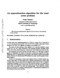
(a) Execution time

Figure 2: The execution time and cost of the returned solution for GA and CSPP. AI: Average Improvement (over 90 executions in 3 environments) of CSPP in comparison with GA, std of GA: average of standard deviation (over 90 executions in 3 environments) the returned solution, average standard deviations of execution time and cost of the solution for GA, and the average improvement (AI) of the CSPP in comparison with GA. CSPP is a deterministic algorithm therefore the variance of its execution time and variance of solution cost are zero for all experiments and thus not reported. According to this figure, CSPP improves the results both in terms of the execution time and cost of the solution. Comparing the outputs of the two algorithms, we get the following results:

any infinite edge. Accordingly, the triangles used in performing confined shortcut (each confined shortcut execution replaces two edges of tour corresponding to a triangle with the third edge of the triangle) do not include any infinite edge. Thus, based on Theorem 2, triangle inequality is not violated in these triangles and in each execution of confined shortcuts (in step 5), the length of the tour decreases. It means that the length of the Hamiltonian tour, h-trail, returned by CSPP is less than the length of trail: ˆ  2W (T ⇤ ). W (h-trail)  W (trail) = W (G)

1. Increasing the number of subpaths causes large deviations in the output of the GA technique. This is often not appealing since one would require multiple executions of GA to avoid sub-optimal results. 2. Fig. 2 indicates that the CSPP algorithm can find better solutions than GA with significantly less computation. More importantly, the differences between two algorithms are intensified for larger graphs, making CSPP a more reliable technique for large-scale problems.

(13)

Hence, the solution produced by CSPP is within 2 of optimum and the ratio bound of CSPP is 2. ⇤

5

(b) Cost of the solution

Experiments and Results

3. The CSPP algorithm is a faster alternative than GA algorithm for solving SPP in all experiments.

In this section, we empirically gauge the performance of CSPP by comparing it with the GA-based method proposed in [Gyorfi et al., 2010]. Throughout this section, we refer to this method by GA. In our experiments, we use different sets of workspaces including 3 environments with 20 subpaths, 3 environments with 50 subpaths and 3 environments with 80 subpaths. The length and the location of the subpaths are chosen randomly. Parameter setting for the operation rates of GA are chosen to be 0.5 for crossover, 0.25 for inversion, 0.25 for rotation, 0.5 for mutation and 0.5 for subpath reversal. These parameters are fixed during all experiments and seem to be near optimal set of parameters, according to the results of different parameter settings. The bar charts in Fig. 2 show the average results of 30 executions (per environment) of CSPP and GA. Fig. 2 also shows the average execution time, average cost (length) of

Our experimental evaluations clearly show the superiority of CSPP over GA for different synthesized environments.

6

Conclusion and Future Work

We presented a 2-approximation algorithm to solve SPP. We addressed the deficiencies of existing meta-heuristic methods for solving SPP by designing a fixed-ratio bound approximation algorithm. Both theoretical and empirical analyses show superiority of CSPP over other existing solutions. We plan to use IETI algorithm with a modified version of RPP [Eiselt et al., 1995a] algorithms to enhance the ratio bound. Acknowledgment We are grateful to anonymous reviewers for their useful comments.

674

References

matching in general graphs. Foundations of Computer Science, pages 17–27, 1980. [Nash et al., 2009] Alex Nash, Sven Koenig, and Maxim Likhachev. Incremental phi*: Incremental any-angle path planning on grids. International Jont Conference on Artifical Intelligence, 2009. [Orloff, 1974] CS Orloff. A fundamental problem in vehicle routing. Networks, 4(1):35–64, 1974. [Papadimitriou, 1977] Christos H Papadimitriou. The euclidean travelling salesman problem is np-complete. Theoretical Computer Science, 4(3):237–244, 1977. [Pemmaraju and Skiena, 2003] S.V. Pemmaraju and S.S. Skiena. Computational discrete mathematics: combinatorics and graph theory with Mathematica. Cambridge Univ Pr, 2003. [Prim, 1957] R.C. Prim. Shortest connection networks and some generalizations. Bell system technical journal, 36(6):1389—1401, 1957. [Safilian et al., 2016] Masoud Safilian, S Mehdi Tashakkori, Sepehr Eghbali, and Aliakbar Safilian. An approximation approach for solving the subpath planning problem. arXiv preprint arXiv:1603.06217, 2016. [Safra and Schwartz, 2006] Shmuel Safra and Oded Schwartz. On the complexity of approximating tsp with neighborhoods and related problems. computational complexity, 14(4):281–307, 2006. [Surynek, 2015] Pavel Surynek. Reduced time-expansion graphs and goal decomposition for solving cooperative path finding sub-optimally. International Conference on Artificial Intelligence, pages 1916–1922, 2015. [Tong-ying et al., 2004] G. Tong-ying, Q. Dao-kui, and D. Zai-li. Research of path planning for polishing robot based on improved genetic algorithm. International Conference on Robotics and Biomimetics, pages 334—338, 2004.

[Arora, 1996] Sanjeev Arora. Polynomial time approximation schemes for euclidean tsp and other geometric problems. Foundations of Computer Science, pages 2–11, 1996. [Christofides, 1976] N. Christofides. Worst-Case analysis of a new heuristic for the travelling salesman problem. Technical report, DTIC Document, 1976. [Coja-Oghlan et al., 2006] Amin Coja-Oghlan, Sven O Krumke, and Till Nierhoff. A heuristic for the stacker crane problem on trees which is almost surely exact. Journal of Algorithms, 61(1):1–19, 2006. [Dumitrescu and Mitchell, 2001] Adrian Dumitrescu and Joseph SB Mitchell. Approximation algorithms for tsp with neighborhoods in the plane. Annual ACM-SIAM symposium on Discrete algorithms, pages 38–46, 2001. [Eiselt et al., 1995a] Horst A Eiselt, Michel Gendreau, and Gilbert Laporte. Arc routing problems, part i: The chinese postman problem. Operations Research, 43(2):231–242, 1995. [Eiselt et al., 1995b] Horst A Eiselt, Michel Gendreau, and Gilbert Laporte. Arc routing problems, part ii: The rural postman problem. Operations Research, 43(3):399–414, 1995. [Frederickson, 1979] Greg N Frederickson. Approximation algorithms for some postman problems. Journal of the ACM (JACM), 26(3):538–554, 1979. [Goldberg, 1989] D.E. Goldberg. Genetic algorithms in search, optimization, and machine learning. Addisonwesley, 1989. [Gyorfi et al., 2010] Julius S Gyorfi, Daniel R Gamota, Swee Mean Mok, John B Szczech, Mansour Toloo, and Jie Zhang. Evolutionary path planning with subpath constraints. Electronics Packaging Manufacturing, IEEE Transactions on, 33(2):143–151, 2010. [Jaillet and Porta, 2013] L´eonard Jaillet and Josep M Porta. Path planning under kinematic constraints by rapidly exploring manifolds. Robotics, IEEE Transactions on, 29(1):105–117, 2013. [Kapadia et al., 2013] Mubbasir Kapadia, Kai Ninomiya, Alexander Shoulson, Francisco Garcia, and Norman Badler. Constraint-aware navigation in dynamic environments. Proceedings of Motion on Games, pages 111–120, 2013. [Kruskal, 1956] J.B. Kruskal. On the shortest spanning subtree of a graph and the traveling salesman problem. Proceedings of the American Mathematical society, 7(1):48— 50, 1956. [Lin and Kernighan, 1973] Shen Lin and Brian W Kernighan. An effective heuristic algorithm for the traveling-salesman problem. Operations research, 21(2):498–516, 1973. [Micali and Vazirani, p 1980] Silvio Micali and Vijay V Vazirani. An O( |V |.|E|) algoithm for finding maximum 675