1
ISAST Transactions on Computers and Intelligent Systems, No. 2, Vol. 1, 2009 A. Javadi et.al: An Artificial Intelligence Based Finite Element Method
An Artificial Intelligence Based Finite Element Method Akbar A. Javadi, Moura Mehravar, Asaad Faramarzi and Alireza Ahangar-Asr
Abstract—In this paper, a new approach is presented based on artificial intelligence and evolutionary computing, for constitutive modeling of materials in finite element analysis, with potential applications in different engineering disciplines. This new approach presents a unified framework for constitutive modeling of complex materials in finite element analysis using evolutionary polynomial regression (EPR). EPR is a data-driven method based on evolutionary computing, aimed to search for polynomial structures representing a system. A procedure is presented for construction of EPRbased constitutive model (EPRCM) and its integration in finite element procedure. The main advantage of EPRCM over conventional and neural network-based constitutive models is that it provides the optimum structure for the material constitutive model representation as well as its parameters, directly from raw experimental (or field) data. It can learn nonlinear and complex material behavior without any prior assumption on the constitutive relationship. The proposed approach provides a transparent relationship for the constitutive material model that can readily be incorporated in a finite element model. A procedure is presented for efficient training of EPR, computing the stiffness matrix using the trained EPR model and incorporation of the EPRCM in a commercial finite element code, ABAQUS. The application of the developed EPR-based finite element method is illustrated through two examples and advantages of the proposed method over conventional and neural network-based FE methods are highlighted. Index Terms— Constitutive Modeling, Data Mining, Evolutionary Computation, Finite Elements
Manuscript received November 2, 2009. Akbar A. Javadi is a Senior Lecturer in Geotechnical Engineering in University of Exeter, School of Engineering, Mathematics and Physical Sciences, Exeter, EX4 4QF, UK (corresponding author; phone: +44 1392 263640; fax: +44 1392 217965; e-mail:
[email protected]). Moura Mehravar is an MSc student in Civil Engineering, Department of Civil Engineering in Azad University, South Tehran Branch, Tehran, Iran, (e-mail:
[email protected]). Asaad Faramarzi is a PhD student in Geotechnical Engineering in University of Exeter, School of Engineering, Mathematics and Physical Sciences, Exeter, EX4 4QF, UK (e-mail:
[email protected]). Alireza Ahangar-Asr is a PhD student in Geotechnical Engineering in University of Exeter, School of Engineering, Mathematics and Physical Sciences, Exeter, EX4 4QF, UK (e-mail:
[email protected]).
S
I. INTRODUCTION
imulation techniques, and in particular the finite element method, have been used successfully to predict the response of systems across a whole range of industries including aerospace and automotive, biomedical, chemical processes, geotechnical engineering and many others. In this numerical analysis the behavior of the actual material is approximated with that of an idealized material that deforms in accordance with some constitutive relationships. Therefore, the choice of an appropriate constitutive model that adequately describes the behavior of the material plays an important role in the accuracy and reliability of the numerical predictions. During the past few decades several constitutive models have been developed for various materials. Most of these models involve determination of material parameters, many of which have a little physical meaning [1]. Despite considerable complexities of constitutive theories, due to the erratic and complex nature of some materials such as soils, rocks, composites, etc., none of the existing constitutive models can completely describe the real behavior of these materials under various stress paths and loading conditions. In conventional constitutive modeling, an appropriate mathematical model is initially selected and the parameters of the model (material parameters) are identified from appropriate physical tests on representative samples to capture the material behavior. When these constitutive models are used in finite element analysis, the accuracy with which the selected material model represents the various aspects of the actual material behavior affects the accuracy of the finite element prediction. In the past few decades, attempts have been made by a number of researchers to use artificial neural networks (ANN) to model the constitutive material behavior. The application of ANN for constitutive modeling of concrete was first proposed by Ghaboussi et al. [2]. Ghaboussi and Sidarta [3] presented an improved technique of ANN approximation for learning the mechanical behavior of drained and undrained sand. The role of ANN in constitutive modeling was also studied by a number of other researchers (e.g., [4-9]). These studies indicated that neural network-based constitutive models can capture nonlinear material behavior with high accuracy. While it has been shown that ANNs offer great advantages in constitutive
2
ISAST Transactions on Computers and Intelligent Systems, No. 2, Vol. 1, 2009 A. Javadi et.al: An Artificial Intelligence Based Finite Element Method
modeling of materials, they also have some drawbacks. One of the main disadvantages of the NNCM is that the optimum structure of the ANN (e.g., number of layers, number of neurons in the hidden layers, transfer functions, etc.) must be identified a priori which is usually obtained using a time consuming trial and error procedure. Another drawback of the NNCM approach is the large complexity of the network structure as it represents the knowledge in terms of a weight matrix and biases that are not accessible to user [10]. Although one of the main applications of material modeling is in numerical analysis of boundary value problems, to date not many researchers have considered the integration of the neural network based constitutive models (NNCMs) in numerical modeling techniques such as finite element method [1]. The main reason for this appears to be the fact that there are considerable difficulties in incorporating a general NNCM in finite element codes [11]. However, more recently it has been shown that NNCM can be practically incorporated in a finite element code as a material model (e.g., [12, 13]). Hashash et al. described some of the issues related to the numerical implementation of a NNCM in finite element analysis and derived a closedform solution for material stiffness matrix for the neural network-based constitutive model [13]. Javadi and his coworkers have carried out extensive research into application of neural networks in constitutive modeling of complex materials. They have developed an intelligent finite element method (NeuroFE code) based on the incorporation of a back propagation neural network (BPNN) in finite element analysis (e.g., [14–17]). In their work, they used actual material test results to extract stress– strain relationship and to train the NNCM. It has been shown that NNCMs trained in this way can be very efficient in learning and generalizing the constitutive behavior of complex materials and give better results (compared with conventional constitutive models) when they are employed in a finite element code to analyse structures or domains made of the material under consideration. In this paper a new approach is introduced for constitutive modeling of complex materials, which integrates numerical and symbolic regression to perform evolutionary polynomial regression (EPR). The strategy uses polynomial structures to take advantage of their favorable mathematical properties. The main idea behind the EPR is to use evolutionary search for exponents of polynomial expressions by means of a genetic algorithm (GA) engine. This allows (i) easy computational implementation of the algorithm, (ii) efficient search for an explicit expression (formula) and (iii) improved control of the complexity of the expression generated [18]. In what follows, the main principles of EPR will be outlined. A procedure is presented for computing the stiffness matrix using the trained EPR model and incorporation of the EPRCM in the finite element software ABAQUS. The application of the developed EPR-based finite element
method is illustrated through two examples. II. EVOLUTIONARY POLYNOMIAL REGRESSION Evolutionary polynomial regression (EPR) is a datadriven method based on evolutionary computing, aimed to search for polynomial structures representing a system. A general EPR expression can be presented as [18]: n
y = ∑ F ( X , f ( X ), a j ) + a0
(1)
j =1
where y is the estimated vector of output of the process;
a j is a constant; F is a function constructed by the process; X is the matrix of input variables; f is a function defined by the user and n is the number of terms of the target expression. The general functional structure represented by F ( X , f ( x ), a j ) + a0 is constructed from elementary functions by EPR using a (GA) strategy. The GA is employed to select the useful input vectors from X to be combined. The building blocks (elements) of the structure of F are defined by the user based on understanding of the physical process. While the selection of feasible structures to be combined is done through an evolutionary process, the parameters a j are estimated by the least square method. EPR is a technique for data-driven modeling. In this technique, the combination of the genetic algorithm to find feasible structures and the least square method to find the appropriate constants for those structures implies some advantages. In particular, the GA allows a global exploration of the error surface relevant to specifically defined objective functions. By using such objective (cost) functions some criteria can be selected to be satisfied through the search process. These criteria can be set in order to (i) avoid the overfitting of models, (ii) push the models towards simpler structures, and (iii) avoid unnecessary terms representative of the noise in data. An interesting feature of EPR is in the possibility of getting more than one model for a complex phenomenon. A further feature of EPR is the high level of interactivity between the user and the methodology. The user’s physical insight can be used to make hypotheses on the elements of the target function and on its structure (Eq. (1)). Selecting an appropriate objective function, assuming pre-selected elements in Eq. (1) based on engineering judgment, and working with dimensional information enable refinement of final models. Detailed explanation can be found in [18], [19]. III. CONSTITUTIVE MODELLING USING EPR In constitutive modeling using EPR, the raw experimental or in-situ test data are directly used for training the EPR. In this approach, there are no mathematical models to select and the EPR learns the constitutive relationships directly
ISAST Transactions on Computers and Intelligent Systems, No. 2, Vol. 1, 2009 A. Javadi et.al: An Artificial Intelligence Based Finite Element Method
3
from the raw data during the training process. As a result, there are no material parameters to be identified and as more data becomes available, the material model can be improved by re-training of the EPR using the additional data. Furthermore, the incorporation of an EPR in a finite element procedure avoids the need for complex yielding/failure functions, flow rules, etc. An EPR equation can be incorporated in a finite element code/procedure in the same way as a conventional constitutive model. It can be incorporated either as incremental or total stress-strain strategies. In this study both the incremental and total stressstrain strategies have been successfully implemented in the intelligent finite element model. A. Input and output parameters The choice of input and output quantities is determined by both the source of the data and the way the trained EPR model is to be used. A typical scheme to train most of the neural network based material models includes an input set providing the network with the information relating to the current state units (e.g., current stresses and current strains)
σ = 8.136 × 10¹³ ε 5 − 2.839 × 10¹¹ ε 4 + 3.115 × 10⁸ ε 3
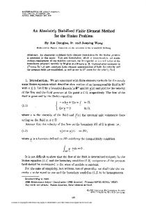
(2) − 8.285 × 10 4 ε 2 + 2.10 × 10¹¹ε − 5.921 × 10⁻³ where ε is the strain and σ is corresponding stress. The second set of data is corresponding to a material with elasto-plastic behavior. After training EPR, Eq. 3 is selected as the best EPR model based on the COD.
250
200 Stress (MPa)
and then a forward pass through the neural network yields the prediction of the next expected state of stress and/or strain relevant to an input strain or stress increment [7]. In this paper, a method is introduced based on EPR for constitutive modeling in finite element analysis. This method takes advantage of the explicit mathematical representation of the relationships in EPR. To evaluate the potential of using EPR to derive functions describing the constitutive behavior of materials two sets of stress-strain data are employed to train and test the EPR models. In both cases the data is divided into two separate sets. One set is used for training of the EPR model and the other one is used for validation to appraise the generalization capability of the trained EPR model. After training and validation, the best function is selected, based on the quality of fit according to the coefficient of determination (COD) and also how well the selected model represents the actual stress-strain behavior. The first set of strain-stress data is representing a material with linear elastic behavior. The selected EPR model for the curve passing through data points is:
150 100
σ = 2.167 × 10¹¹ ε − 6.297 × 10¹⁵ ε 3 +1.034 × 10¹⁸ ε 4
Original Data EPR
− 8.032 × 10¹⁹ ε 5 + 3.441 × 10²¹ ε 6 − 8.024 × 10 22 ε 7
50
+ 8.766 × 10²³ ε 8 − 2.545 × 10 24 ε 9 − 6.505 × 10⁶
(3)
0 0
0.0002
0.0004 0.0006 Strain
0.0008
(a) 1400 1200
Stress (MPa)
1000 800 600 Original Data
400
EPR
200 0 0
0.005
0.01
0.015
0.02
0.025
Strain
(b) Fig. 1. Results of the EPR models prediction and the original data.
0.001
Figs. 1a and 1b show the stress-strain curve predicted by Eqs. 2 and 3 (as a marker points) against those expected. It can be seen from these figures that EPR has successfully captured the material behavior with an excellent accuracy. The material model in an FE analysis has to provide the material stiffness matrix also known as the Jacobian. For infinitesimal strain increments ( dε ), J is the continuum Jacobian, J c
∂ ( dσ ) (4) ∂ ( dε ) This equation will be employed later to build the stiffness matrix. Jc =
IV. INTELLIGENT FINITE ELEMENTS The obtained EPRCMs are implemented in a widely used general-purpose finite element code ABAQUS through the user defined material module (UMAT). UMAT updates the stresses and provides the material Jacobian matrix for every increment at every integration point [20], [21]. In the developed methodology (EPR–FEM), the EPRCM replaces
ISAST Transactions on Computers and Intelligent Systems, No. 2, Vol. 1, 2009 A. Javadi et.al: An Artificial Intelligence Based Finite Element Method
4
the role of a conventional constitutive model. The source of knowledge for EPR is a set of raw experimental (or in situ) data representing the mechanical response of the material to applied load. When EPR is used for constitutive description, the physical nature of the input–output data for the EPR is clearly determined by the measured quantities, e.g., stresses, strains, etc. The manner, in which EPRCM is
incorporated in a FE code, is described in Fig. 2. This figure also shows the main steps of EPR. The constitutive relationship are generally given in the form [22]
∆σ = D∆ε
EPR
(5)
FEA Start
Start
Input Data (Geometry, Applied Load, Initial and Boundary Condition)
Input Data (Experimental Data, Physical Insight)
Increase the Applied Load Incrementally
Current state of stresses and strains Load Increment Loop
Genetic Algorithm
UMAT EPRCM(s)
Mathematical Structure
1- Next state of Stresses 2- Jacobian Matrix
EPR Constitutive equation
Iteration Loop
Least Square
Solve the Main Equation
NO
Symbolic Function
Convergence
YES
Fitness
NO
Output Result
YES
Whole load applied?
NO
Check based on fitness criteria and or generation number YES
STOP
Fig. 2. The incorporation of EPR-based material model in ABAQUS finite element software for an integration point.
ISAST Transactions on Computers and Intelligent Systems, No. 2, Vol. 1, 2009 A. Javadi et.al: An Artificial Intelligence Based Finite Element Method
where D is material stiffness matrix also known as the Jacobian. Assuming that matrix is elastic and isotropic for a load increment, matrix D is given in terms of Young’s modulus, E, and Poisson’s ratio, ν. For a plane strain case, for example
ν ν 1 − ν ν ν ν 1 − E D= ν ν 1 −ν (1 + ν )(1 − 2ν ) 0 0 0
0
1 − 2ν 2
0 0
The EPR-based finite element model incorporating the trained EPR was used to analyse the behavior of the cylinder under applied internal pressure. Assuming a linear behavior for a small load increment in the nonlinear FE analysis, the tangential elastic modulus of the material at each strain can be obtained from the derivative of the Eq. 2. Therefore the EPR based elastic modulus can be taken as: Et =
(6)
A. Numerical Examples 1) Example 1: This example involves a thick circular cylinder conforming to plane strain conditions. Fig. 3 shows the geometric dimensions and the element discretization employed in the solution and it is seen that 12 parabolic isoparametric elements have been used. The cylinder is made of linear elastic material with a Young's modulus of E=2.1×10⁵ N/mm2 and a Poisson's ratio of 0.3 [22]. This example was deliberately kept simple in order to verify the computational methodology by comparing the results of a linear elastic finite element model. The loading case considered involves an internal pressure of 8.0×10⁴ kN with boundary conditions as shown in Fig. 3.
dσ = 4.068 × 10¹⁴ ε 4 − 1.1356 × 10¹² ε 3 dε + 9.345 × 10⁸ ε 2 − 1.657 × 10⁵ ε + 2.1 × 10¹¹
(7)
Eq. 7 is used to calculate stiffness matrix (Eq. 6). During the analysis, the Poisson’s ratio was kept constant.
200
160 Standard FEM
Stress (MPa)
5
IFEM (EPRCM)
120
80
40
0 0
40
80
120
160
200
r (mm)
(a)
Radial Displacement (mm)
0.08
P
0.06 Standard FEM IFE (EPRCM)
0.04
0.02
0 0
40
80
120
160
200
r (mm)
100 mm
(b) 200 mm
Fig. 3. FE Mesh in symmetric quadrant of a thick cylinder.
Fig. 4. Comparison of the results of the EPR-FEM and standard FEM in terms of (a) radial stress and (b) radial displacement
ISAST Transactions on Computers and Intelligent Systems, No. 2, Vol. 1, 2009 A. Javadi et.al: An Artificial Intelligence Based Finite Element Method
6
The results are compared with those obtained using a standard linear elastic finite element method. Fig. 4 shows the radial displacements and radial stresses along a radius of the cylinder, predicted by the two different methods. Comparison of the results shows that the results obtained using the EPR based FEM are in excellent agreement with those attained from the standard finite element analysis. This shows the potential of the developed EPR based finite element method in deriving constitutive relationships from raw data using EPR and using these relationships to solve boundary value problems. 2) Example 2: The second example is a plane stress beam (Fig. 5) subjected to uniform pressure. The developed EPR constitutive model (Eq. 3) is used to describe the material behavior. To evaluate the described methodology, displacement of point A (mid-span) of the beam predicted using the EPR-based FE analysis is compared with that from conventional FE analysis. For the conventional FE analysis, an elasto-plastic model in ABAQUS, based on the tabulated stress-strain data, is used. For the EPR-based FE analysis, the Young’s modulus is determined as: Et =
dσ = 2.167 × 10¹¹ − 1.889 × 10¹⁶ ε 2 + 4.137 × 10¹⁸ ε 3 dε − 4.016 × 10²⁰ ε 4 + 2.064 × 10²² ε 5 − 5.616 × 10 23 ε 6 + 7.013 × 10 ε − 2.272 × 10 ε 24
7
25
(8)
8
Fig. 6 shows the load-displacement curves at point A (mid-span of the beam) obtained using the conventional FE model and the developed EPR-based FE model. It is shown that results of the EPR-based FEM are in very good agreement with those from the conventional FE analysis using an elasto-plastic model.
Applied Pressure (MPa)
50 40 30 20 Elasto_Plastic FE Analysis EPRCM FE Analysis
10 0 0
1
2
3
4
5
displacement (mm)
Fig. 6. Comparison of the results of the EPR-based FEM and conventional FEM
V. CONCLUSIONS An intelligent finite element method (EPR-FEM) has been developed based on the integration of an EPRCM in a finite element framework. In the developed methodology, the EPRCM is used as an alternative to the conventional constitutive models for the material. A procedure is presented for computing the stiffness matrix using the trained EPR model and incorporation of the EPRCM in a commercial finite element code ABAQUS. The efficiency and adaptability of the proposed method have been demonstrated by successful application to two boundary value problems. The results of the analysis have been compared to those obtained from conventional FE analyses using the linear elastic and elastic-plastic models. The result shows that EPRCM can be successfully implemented in a finite element model as an effective alternative to conventional material models. It is also shown that stiffness matrix elements can be directly obtained from EPR stressstrain relationship. REFERENCES [1]
100 mm
[2]
A 600 mm Fig. 5. Simply supported beam under uniform pressure
[3] [4] [5] [6] [7]
H.S. Shin, Neural network based constitutive models for finite element analysis, PhD Dissertation, University of Wales, Swansea, UK, 2001. J. Ghaboussi, J. Carret and X. Wu, Knowledge-based modeling of material behavior with neural networks. Journal of Engineering Mechanics Division, vol. 17, pp. 32-153, 1991. J. Ghaboussi and D.E. Sidarta, New nested adaptive neural networks (NANN) for constitutive modeling. Computers and Geotechnics, vol. 22, pp. 29-52, 1998. D. Penumadu and R. Zhao, Triaxial compression behavior of sand and gravel using artificial neural networks. Computers and Geotechnics, vol. 24, pp. 207-230, 1999. G.W. Ellis, C. Yao, R. Zhao, D. Penumadu, Stress–strain modeling of sands using artificial neural netwoks, ASCE Journal of Geotechnical Engineering Division vol. 121, pp. 429–435, 1995. J.-H. Zhu, M.M. Zaman, S.A. Anderson, Modeling of soil behavior with a recurrent neural network, Canadian Geotechnical Journal vol. 35, pp. 858–872, 1998. J. Ghaboussi, D.A. Pecknold, M. Zhang, R.M. Haj-Ali, Autoprogressive training of neural network constitutive models,
7
[8] [9]
[10] [11]
[12] [13]
[14] [15]
[16] [17]
[18] [19] [20] [21] [22]
ISAST Transactions on Computers and Intelligent Systems, No. 2, Vol. 1, 2009 A. Javadi et.al: An Artificial Intelligence Based Finite Element Method
International Journal for Numerical Methods in Engineering vol. 42, pp. 105–126, 1998. D.E. Sidarta, J. Ghaboussi, Constitutive modeling of geomaterials from nonuniform material tests, Computers and Geotechnics vol. 22,pp. 53–71,1998. D. Penumadu, J.L. Chameau, Geomaterial modeling using neural networks, in: N. Kartman, I. Flood, J.H. Garrett (Eds.), Artificial Neural Networks for Civil Engineering: Fundamentals and Applications, ASCE, 1997, pp. 160–184. A.A. Javadi and M. Rezania. Applications of artificial intelligence and data mining techniques in soil modeling. Geomechanics and Engineering, an International Journal, vol. 1, pp. 53-74, 2009. H.S. Shin, G.N. Pande, Enhancement of data for training neural network based constitutive models for geomaterials, in: Proceedings of the Eighth International Symposium on Numerical Models in Geomechanics-NUMOG VIII, Rome, Italy, pp. 141–146, 2002. H.S. Shin and G.N. Pande, On self-learning finite element code based on monitored response of structures. Computers and Geotechnics, vol. 27, pp. 161-178, 2000. Y.M. Hashash, S. Jung and J. Ghaboussi, Numerical implementation of a neural network based material model in finite element analysis. Int. Journal for Numerical Methods in Engineering, vol. 5, pp. 9891005 2004. A.A. Javadi, T.P. Tan and M. Zhang, Neural network for constitutive modeling in finite element analysis. Computer Assisted Mechanics and Engineering Sciences, vol. 10, pp. 375-381, 2003. A.A. Javadi, M. Zhang, T.P. Tan, Neural network for constitutive modeling of material in finite element analysis, in: Proceedings of the Third International Workshop/Euroconference on Trefftz Method, Exeter, UK, pp. 61–62, 2002. A.A. Javadi, T.P. Tan, A.S.I. Elkassas, An intelligent finite element method, in: Proceedings of the 11th International EG-ICE Workshop, Weimar, Germany, pp. 16–25, 2004. A.A. Javadi, T.P. Tan, A.S.I. Elkassas, Intelligent finite element method, in: Proceedings of the Third MIT Conference on Computational Fluid and Solid Mechanics, Cambridge, Massachusetts, USA, pp. 347–350, 2005. O. Giustolisi and D.A. Savic. A Symbolic Data-driven Technique Based on Evolutionary Polynomial Regression. Journal of Hydroinformatics, vol. 8, pp. 207–222, 2006. A. Doglioni, O. Giustolisi, D.A. Savic, B.W. Webb, An investigation on stream temperature analysis based on evolutionary computing, Hydrological Processes vol. 22, pp. 315–326, 2008. ABAQUS User Subroutines Reference Manual (version 6.7-1) Dassault Systems, 2007. ABAQUS Theory Manual (version 6.7-1) Dassault Systems, 2007. D.R.J. Owen, E. Hinton, Finite Elements in Plasticity: Theory and Practice, Pineridge Press, Swansea, 1980.