An Assessment of Call Graph Construction Algorithms

RC 21699 (97756) 22 March 2000

Computer Science/Mathematics

IBM Research Report An Assessment of Call Graph Construction Algorithms

David Grove IBM T.J. Watson Research Center P.O. Box 704 Yorktown Heights, NY 10598

Craig Chambers Department of Computer Science and Engineering University of Washington P.O. Box 352350 Seattle, WA 98195

LIMITED DISTRIBUTION NOTICE: This report has been submitted for publication outside of IBM and will probably be copyrighted if accepted for publication. It has been issued as a Research Report for early dissemination of its contents. In view of the transfer of copyright to the outside publisher, its distribution outside of IBM prior to publication should be limited to peer communications and specific requests. After outside publication, requests should be filled only by reprints or legally obtained copies of the article (e.g., payment of royalties). Copies may be requested from IBM T.J.Watson Research Center P.O. Box 218, Yorktown Heights, NY 10598 USA. Some reports are available on the internet at http://domino.watson.ibm.com/library/ CyberDig.nsf/home.

2

An Assessment of Call Graph Construction Algorithms David Grove

Craig Chambers

IBM T.J. Watson Research Center P.O. Box 704, Yorktown Heights, NY 10598 [email protected]

Department of Computer Science and Engineering University of Washington P.O. Box 352350, Seattle, WA 98195 [email protected]

Abstract A large number of call graph construction algorithms for object-oriented and functional languages have been proposed, each embodying different tradeoffs between analysis cost and call graph precision. In this paper, we present a unifying framework for understanding call graph construction algorithms and an empirical comparison of a representative set of algorithms. We first present a general parameterized algorithm that encompasses many well-known and novel call graph construction algorithms. We have implemented this general algorithm in the Vortex compiler infrastructure, a mature, multi-language, optimizing compiler. The Vortex implementation provides a “level playing field” for meaningful cross-algorithm performance comparisons. The costs and benefits of a number of call graph construction algorithms are empirically assessed by applying their Vortex implementation to a suite of sizeable (5,000 to 50,000 lines of code) Cecil and Java programs. For many of these applications, interprocedural analysis enabled substantial speed-ups over an already highly optimized baseline. Furthermore, a significant fraction of these speed-ups can be obtained through the use of a scalable, near-linear time call graph construction algorithm.

1 Introduction Frequent procedure calls and message sends serve as important structuring tools for object-oriented languages. However, they can also severely degrade application run-time performance. This degradation is due both to the direct cost of implementing the call and to the indirect cost of missed opportunities for compile-time optimization of the code surrounding the call. A number of techniques have been developed to convert message sends into procedure calls (to statically bind the message send) and to inline statically bound calls, thus removing both the direct and indirect costs of the call. However, in most programs, even after these techniques have been applied there will be some remaining non-statically bound message sends and non-inlined procedure calls. If the presence of these call sites force an optimizing compiler to make overly pessimistic assumptions, then potentially profitable optimization opportunities can be missed leading to significant reductions in application performance. Interprocedural analysis is one method for enabling an optimizing compiler to more precisely model the effects of noninlined calls, thus enabling it to make less pessimistic assumptions about program behavior and reduce the performance impact of non-inlined call sites. An interprocedural analysis can be divided into two logically separate sub-tasks. First, the program call graph, a compile-time data structure that represents the run-time calling relationships among a program’s procedures, is constructed. In most case this will be done as an explicit pre-phase before performing the “real” interprocedural analysis, although some analyses will interleave call graph construction and analysis and others may only construct the call graph implicitly. Second, the “real” analysis is performed by traversing the call graph to compute summaries of the effect of callees at each call site and/or summaries of the effect of callers at each procedure entry. These summaries are then consulted when compiling and optimizing individual procedures. In strictly first-order procedural languages, constructing the program call graph is straightforward; at every call site the target of the call is directly evident from the source code. However in object-oriented languages or languages with function values, the target of a call cannot always be precisely determined solely by an examination of the source code of the call site. In these languages, the target procedures invoked at a call site are at least partially determined by the

1

An Assessment of Call Graph Construction Algorithms

Grove and Chambers

data values that reach the call site. In object-oriented languages, the method invoked by a dynamically dispatched message send depends on the class of the object receiving the message; in languages with function values, the procedure invoked by the application of a computed function value depends on the value of the function value. In general, determining the flow of values needed to build a useful call graph requires an interprocedural data and controlflow analysis of the program. But, interprocedural analysis in turn requires that a call graph be built prior to the analysis being performed. This circular dependency between interprocedural analysis and call graph construction is the key technical difference between interprocedural analysis of object-oriented and functional languages and interprocedural analysis of strictly first-order procedural languages. Effectively resolving this circularity is the primary challenge of the call graph construction problem for object-oriented languages. The main contributions of this work are: • A general parameterized algorithm for call graph construction is developed. The general algorithm provides a uniform vocabulary for describing call graph construction algorithms, illuminates their fundamental similarities and differences, and enables an exploration of the algorithmic design space. The general algorithm is quite expressive, encompassing algorithms with a wide range of cost and precision characteristics. • The general algorithm is implemented in the Vortex compiler infrastructure. The definition of the general algorithm naturally gives rise to a flexible implementation framework that enables new algorithms to be easily implemented and assessed. Implementing all of the algorithms in a single framework incorporated in a mature optimizing compiler provides a “level playing field” for meaningful cross-algorithm performance comparisons. • A representative selection of call graph construction algorithms is experimentally assessed. The Vortex implementation framework is used to test each algorithm on a suite of sizeable (5,000 to 50,000 lines of code) Cecil and Java programs. In comparison to previous experimental studies, our experiments cover a much wider range of algorithms and include applications that are an order of magnitude larger than the largest used in prior work. Assessing the algorithms on larger programs is important because some of the algorithms, including one that previous work has claimed is scalable, cannot be practically applied to some of our larger benchmarks. This paper is organized into two major parts: a presentation of our general parameterized call graph construction algorithm (Sections 2 through 5) and an empirical assessment of a representative set of instantiations of the general algorithm (Sections 6 through 11). Section 2 begins by reviewing the role of class analysis in call graph construction. Sections 3 and 4 are the core of the first half of the paper; they formally define call graphs and the call graph construction problem and present our general parameterized algorithm. Section 5 describes our implementation of the algorithm in the Vortex compiler infrastructure: it focuses on our design choices and how key primitives are implemented. Section 6 begins the second half of the paper by describing our experimental methodology. Sections 7 through 10 each describe and empirically evaluate a category of call graph construction algorithms. Section 11 concludes the second half of the paper by summarizing our experimental results. Finally Section 12 discusses some additional related work and Section 13 concludes.

2 The Role of Interprocedural Class Analysis In object-oriented languages, the potential target method(s) of many calls cannot be precisely determined solely by an examination of the source code of their call sites. The problem is that the target methods that will be invoked as a result of the message send are determined by the classes of the objects that reach the message send site at run-time and thus act as receivers for the message. In general, the flow of objects to call sites may be interprocedural and thus precisely determining the receiver class sets needed to build the call graph requires an interprocedural data and control-flow analysis of the program. But, interprocedural analysis in turn requires that a call graph be built prior to the analysis being performed. There are two possible approaches for handling the circular dependencies between receiver class sets, the program call graph, and interprocedural analysis:

2


Grove and Chambers

• by making a pessimistic (but sound) assumption: This approach breaks the circularity by making a conservative assumption for one of the three quantities and then computing the other two. For example, a compiler could perform no interprocedural analysis, assume that all statically type-correct receiver classes are possible at every call site, and in a single pass over the program construct a sound call graph. Similarly, intraprocedural class analysis could be performed within each procedure (making conservative assumptions about the interprocedural flow of classes) to slightly improve the receiver class sets before constructing the call graph. This overall process can be iteratively repeated to further improve the precision of the final call graph by using the current pessimistic solution to make a new, pessimistic assumption for one of the quantities and then using the new approximation to compute a better, but still pessimistic, solution. Although the simplicity of this approach is attractive, it may result in call graphs that are too imprecise to enable effective interprocedural analysis. • by making an optimistic (but likely unsound) assumption and iterating to fix-point: Just like in the pessimistic approach, an initial guess is made for one of the three quantities giving rise to values for the other two quantities. The only fundamental difference is that because the initial guess may have been unsound, after the initial values are computed further rounds of iteration may be required to reach a fix-point. As an example, many call graph construction algorithms make the initial optimistic assumption that all receiver class sets are empty and that the main routine* is the only procedure in the call graph. Based on this assumption, the main routine is analyzed and in the process it may be discovered that in fact other procedures are reachable and/or some class sets contain additional elements, thus causing further analysis to be required. The optimistic approach can yield more precise call graphs (and receiver class sets) than the pessimistic approach, but is more complicated and may be more computationally expensive. This paper presents and empirically assesses call graph construction algorithms that utilize both of the approaches. The data demonstrate that call graphs constructed by algorithms based on the first (pessimistic) approach are substantially less precise than those constructed by algorithms that utilize the second (optimistic) approach. Furthermore, these precision differences impact the effectiveness of client interprocedural analyses and in turn substantially impact bottom-line application performance. Therefore, Sections 3 and 4 concentrate on developing formalisms that naturally support describing optimistic algorithms that integrate call graph construction and interprocedural class analysis (although the formalisms can also describe some pessimistic algorithms).

3 A Lattice Theoretic Model of Call Graphs This section precisely defines the output domain of the general integrated call graph construction and interprocedural class analysis algorithm. Section 3.1 informally introduces some of the key ideas. Section 3.2 formalizes the intuition of Section 3.1 using ideas drawn from lattice theory. Finally, Section 3.3 presents some applications of the call graph formalism by using it to discuss algorithmic termination, call graph soundness, and the relationship between the call graph formalism and the definition of the general algorithm presented in Section 4.

3.1

Informal Model of Call Graphs

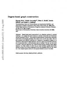
In its standard formulation, a call graph consists of nodes, representing procedures, that are linked by directed edges, representing calls from one procedure to another. However, this formulation is insufficient to accurately capture the output of a context-sensitive interprocedural class analysis algorithm. Instead, each call graph node will represent a contour: an analysis-time specialization of a procedure. In context-insensitive call graphs, there is exactly one contour for each procedure; in context-sensitive call graphs, there may be an arbitrary number of contours representing different analysis-time views of a single procedure. Figure 1(b) shows the context-insensitive call graph for the example program from Figure 1(a). Figure 1(c) depicts the call graph constructed by a context-sensitive algorithm that has separated the integer and float dataflow by creating two contours for the max procedure.

* We

define the main routine of a program to be the union of all program entry points and static data initializations.

3

An Assessment of Call Graph Construction Algorithms procedure main() { return A() + B() + C(); } procedure return } procedure return } procedure return }

Grove and Chambers

main

main

A() { max(4, 7); A

B

C

A

B

C

B() { max(4.5, 2.5); C() { max(3, 1);

(a) Example Program

max

(b) Context-Insensitive

max0

max1

(c) Context-Sensitive

Figure 1: Context-insensitive vs. context-sensitive call graph

Each contour intuitively contains five primary components: • Procedure identifier: identifies which source-level procedure the contour is specializing. • Contour key: encodes the context-sensitivity decisions made during interprocedural class analysis. • Class sets: represent the result of interprocedural class analysis. Every contour contains class sets for formal parameters, local variables, and the procedure’s result. These sets of classes represent the possible classes of objects stored in the corresponding variable (or returned from the procedure) during program execution. • Call graph edges: record for each call site a set of possible callee contours. • Lexical parent contour(s): allow contours representing lexically nested procedures to access the class sets of free variables from the appropriate contour(s) of the enclosing procedure. Intuitively, the first two components of a contour identify it. The third and fourth components record that portion of the final analysis results (class sets and call graph edges) that are local to the contour. The fifth component is only important for languages that allow lexically nested functions and is used to encode the lexical nesting relationship of contours. In addition to the “normal” contours created to represent procedures, special contours can be created to represent other program constructs. For example, a “root” contour can be created to represent the global scope: its local variables are the program’s global variables and its body is the program’s main routine. Interprocedural class analysis also needs to record sets of possible classes for each instance variable, in a manner similar to the class sets for local variables recorded in procedure contours. Array classes are supported by introducing a single instance variable per array class to model the elements of the array. Instance variable contours intuitively consist of three main components: • Instance variable identifier: identifies which source-level instance variable the contour is specializing. • Contour key: just like the contour key component of procedure contours, this field encodes the context-sensitivity decisions made by the interprocedural class analysis algorithm. • Class set: represents the potential classes of values stored in the instance variable. Just like procedure contours, the components of an instance variable contour can be viewed as playing one of two roles: identifying the contour or recording local analysis results. To more precisely analyze polymorphic data structures, some interprocedural class analysis algorithms introduce additional context-sensitivity in their analysis of classes and instance variable contents. Because array classes are

4


Grove and Chambers

modeled just like any other class, the analysis of polymorphic array classes can also benefit from any such contextsensitivity scheme. For example, by treating different instantiation sites of a class as leading to distinct (analysis-time) classes with distinct instance variable contours, an analysis can simulate the effect of templates or parameterized types without relying on explicit parameterization in the source program. Thus a single source-level class may be represented during analysis by multiple class contours. Class contours consist of two components: • Class identifier: identifies the source-level class that the contour is specializing. • Contour key: as with the other contour key components, this field encodes context-sensitivity decisions made by the interprocedural class analysis algorithm. All previously described class information, for example the class sets recorded in procedure and instance variable contours, is generalized to be class contour information. Informally, the result of the combined call graph construction and interprocedural class analysis algorithm defined in Section 4 is a set of procedure contours and a set of instance variable contours. Together, the contents of these two sets define a contour call graph (the call graph edges component of the procedure contours) and class contour sets for all interesting program constructs (the class set component of the procedure and instance variable contours).

3.2

Formal Model of Call Graphs

This subsection uses lattice-theoretic ideas to formally define the contour-based model of context-sensitive call graphs. A lattice D = 〈 S D, ≤ D〉 is a set of elements SD and an associated partial ordering ≤ D of those elements such that for every pair of elements the set contains both a unique least-upper-bound element and a unique greatest-lower-bound element. A downward semilattice is like a lattice but only greatest-lower-bounds are required. The set of possible call graphs for a particular input program and call graph construction algorithm pair forms a downward semilattice; in this paper the term “domain” will be used as shorthand for a downward semilattice. As is traditional in dataflow analysis [Kild73, Kam76] (but opposite to the conventions used in abstract interpretation [Cous77]), if A ≤ B then B represents a better (more optimistic) call graph than A. Thus, the top lattice element, T, represents the best possible (most optimistic) call graph, while the bottom element, ⊥, represents the worst possible (most conservative) call graph. Not all elements of a call graph domain will be sound (safely approximate the “real” program call graph); Section 3.3.2 formally defines soundness and some of the related structure of call graph domains. 3.2.1

Supporting Domain Constructors

The definition of the call graph domain uses several auxiliary domain constructors to abstract common patterns, thus making it easier to observe the fundamental structure of the call graph domain. Some readers may want to skip ahead to Section 3.2.2 to see how the constructors are used before reading the remainder of this section. The constructor Pow maps an input partial order D = 〈 S D, ≤ D〉 to a lattice DPS = 〈 S DPS, ≤ DPS〉 where SDPS is a subset

of

the

powerset

of

SD

defined

as

S DPS =

Bottoms(S) = { d ∈ S ¬( ∃d' ∈ S, d'≤ D d ) } . The partial order ≤ DPS

∪

S ∈ PowerSet ( S D )

Bottoms(S)

is defined in terms of

where ≤D

as:

dps 1 ≤ DPS dps 2 ≡ ∀d 2 ∈ dps 2 , ∃d 1 ∈ dps 1 such that d 1 ≤ D d 2 . If S1 and S2 are both elements of SDPS, then their greatest lower bound is Bottoms(S 1 ∪ S 2) . Pow subtly differs from the standard powerset domain constructor, which maps an input set to a lattice whose domain is the full powerset of its input with a partial order based solely on the subset relationship. The more complex definition of Pow preserves the relationships established by its input partial order. Intuitively, Bottoms(S) serves to remove those elements which are redundant with respect to ≤d from S. Each member of the family of constructors kTuple, ∀k ≥ 0 , is the standard k-tuple constructor which takes k input partial orders D i = 〈 S i, ≤ i〉 , ∀i∈[1..k], and generates a new partial order T = 〈 S T , ≤ T 〉 where ST is the cross product

5


Grove and Chambers

of the Si and ≤ T is defined in terms of the ≤ i pointwise 〈 d 11, …, d k1〉 ≤ T 〈 d 12, …, d k2〉 ≡ ∀i ∈ [ 1..k ] , d i1 ≤ i d i2 . If the input partial orders are downward semilattices, then T is also a downward semilattice; the greatest lower bound of two tuples is the tuple of the pointwise greatest lower bounds of their elements. The constructor Map is a function constructor which takes as input a set X and a partial order Y = 〈 S Y , ≤ Y 〉 and generates a new partial order M = 〈 S M , ≤ M 〉 where S M = { f ⊆ X × S Y (x,y 1) ∈ f ∧ (x,y 2) ∈ f ⇒ y 1 = y 2 } and the partial order ≤ M is defined in terms of ≤ Y as m 1 ≤ M m 2 ≡ ∀(x,y 2) ∈ m 2 , ∃(x,y 1) ∈ m 1 such that y 1 ≤ Y y 2 . If the partial order Y is a downward semilattice, then M is also a downward semilattice; if m1 and m2 are both elements of SM, then their greatest lower bound is GLB 1 ∪ GLB 2 ∪ GLB 3 where: GLB 1 = { (x,y) (x,y 1) ∈ m 1, (x,y 2) ∈ m 2, y = glb(y 1, y 2) } GLB 2 = { (x,y) (x,y) ∈ m 1, x ∉ dom(m 2) } GLB 3 = { (x,y) (x,y) ∈ m 2, x ∉ dom(m 1) } Finally, the constructor AllTuples takes an input downward semilattice D = 〈 S D, ≤ D〉 and generates a downward semilattice V = 〈 S V , ≤ V 〉 by lifting the union of the k-tuple domains of D. The elements of SV are ⊥, all elements of 1Tuple(D) , 2Tuple(D, D) , 3Tuple(D, D, D) , etc., and the partial order ≤V is the union of the individual k-tuple partial orders with the partial order { ( ⊥, e ) e ∈ S V} . If m1 and m2 are both elements of SV and are both drawn from the same k-tuple domain of D, then their greatest lower bound is the greatest lower bound from that domain, otherwise their greatest lower bound is ⊥. 3.2.2

Call Graph Domain

Figure 2 utilizes the domain constructors specified in the previous section to define the call graph domain for a particular input program and call graph construction algorithm pair. This definition is parameterized by inputs that encode program features and algorithm-specific context-sensitivity polices. Program features are abstracted into seven unordered sets: Class is the set of source-level class declarations, InstVariable is the set of source-level instance variable declarations, Procedure is the set of source-level procedure declarations, Variable is the set of all program variable names, CallSite is the set of all program call sites, LoadSite is the set of source-level loads of instance variables, and StoreSite is the set of source-level stores to instance variables. The algorithm-specific information that encodes its context-sensitivity policies is represented by three partial orders: ProcKey, InstVarKey, and ClassKey. The ProcKey parameter defines the space of possible contexts for context-sensitive analysis of functions, i.e., procedure contours. The InstVarKey parameter defines the space of possible contexts for separately tracking the contents of instance variables, i.e., instance variable contours. The ClassKey parameter defines the space of possible contexts for context-sensitive analysis of classes, i.e., class contours. The ordering relation on these partial orders (and all derived domains) indicates the relative precision of the elements: one element is less than another if and only if it is less precise (more conservative) than the other. The two components of a call graph are instance variable contours and procedure contours. Instance variable contours enable the analysis of dataflow through instance variable loads and stores, and procedure contours are used to represent the rest of the program. The components of these contours serve three functions: • The first component of both instance variable and procedure contours serves to identify the contour by encoding the source level declaration the contour is specializing and the restricted context to which it applies. Each call graph is restricted to contain at most one InstVarContour for each InstVarID and at most one ProcContour for each ProcID. The third component of a ProcID identifies a chain of lexically enclosing procedure contours that is used to analyze references to free variables. For each procedure, the third component of all of its contour’s ProcID’s is restricted to tuples of exactly length n, where n is the lexical nesting depth of the procedure. • The second component of both instance variable and procedure contours records the results of interprocedural class analysis. In instance variable contours, it is simply a class contour set that represents the set of class contours

6

An Assessment of Call Graph Construction Algorithms CallGraph

Grove and Chambers

= 2Tuple(InstVarContourSet, ProcContourSet)

InstVarContourSet = Pow(InstVarContour) InstVarContour

= 2Tuple(InstVarID, ClassContourSet)

InstVarID

= 2Tuple(InstVariable, InstVarKey)

ProcContourSet

= Pow(ProcContour)

ProcContour

= 5Tuple(ProcID, Map(Variable, ClassContourSet), Map(CallSite, Pow(ProcID)), Map(LoadSite, Pow(InstVarID)), Map(StoreSite, Pow(InstVarID)))

ProcID

= 3Tuple(Procedure, ProcKey, Pow(AllTuples(ProcKey)))

ClassContourSet

= Pow(ClassContour)

ClassContour

= 2Tuple(Class, Union(ClassKey, AllTuples(ProcKey))) Figure 2: Definition of call graph domain

stored in the instance variable contour. In procedure contours, it is a mapping from each of the procedure’s local variables and formal parameters to a set of class contours representing the classes of values that may be stored in that variable. The variable mapping also contains an entry for the special token return which represents the set of class contours returned from the contour. • The remaining components of a procedure contour encode the inter-contour flow of data and control caused by procedure calls, instance variable loads, and instance variable stores respectively. The third component, which maps call sites to elements of Pow(ProcID), encodes the traditional notion of call graph edges. The definition of ClassContour is somewhat complicated by the overloading of class contours to represent both objects and closure values. In both cases, the first component identifies the source-level class or closure associated with the contour. For classes, the second component of a class contour will contain an element of the ClassKey domain. For closures, the second component will contain a tuple of ProcKey’s that encode the lexical chain of procedure contours that should be used to analyze any references to free variables contained in the closure. This encoded information is used when procedure contours are created for the closure to initialize the third component of their ProcID’s. For example, the 0-CFA algorithm is the classic context-insensitive call graph construction algorithm for object oriented and functional languages [Shiv88, Shiv91]. It can be modeled by using the single point lattice, {⊥}, to instantiate the ProcKey, InstVarKey, and ClassKey partial orders. Thus, each call graph will have at most one procedure and instance variable contour. Another common context-sensitivity strategy is to create analysis-time specializations of a procedure for each of its call sites (Shivers’s 1-CFA algorithm). This corresponds to instantiating the ProcKey partial order to the Procedure set, and using the single point lattice for InstVarKey and ClassKey. As a final example, the 1-CFA algorithm can be generalized to support the context-sensitive analysis of instance variables by tagging each class with the procedure in which it was instantiated and maintaining separate instance variable contours for each class contour. This context-sensitivity strategy is encoded by using the Procedure set to instantiate the ProcKey and ClassKey partial orders and elements of ClassContour as elements of the InstVarKey partial order.

3.3 3.3.1

Applications Termination

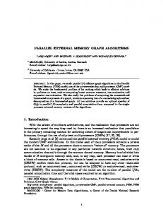
A call graph construction algorithm is monotonic if its computation can be divided into some sequence of steps, S1, S2,…,Sn, where each Si takes as input a call graph Gi and produces a call graph Gi+1 such that G i + 1 ≤cg G i ( ≤cg is

7


Grove and Chambers

GT Optimistic

Gideal Sound

G⊥ Figure 3: Regions in a call graph domain

the call graph partial order defined by the equations of Figure 2). A call graph construction algorithm is bounded-step if each Si is guaranteed to take a finite amount of time. If a call graph construction algorithm is both monotonic and bounded-step and its associated call graph lattice is of finite height,* then the algorithm is guaranteed to terminate in finite time. Furthermore, the worst-case running time of the algorithm is bounded by O(LatticeHeight × StepCost) . All of the sets specifying program features will be finite (since the input program must be of finite size), but the three algorithm-specific partial orders may be either finite or infinite. If the parameterizing partial orders are finite, then the call graph domain will have a finite number of elements and thus a finite height. This result follows immediately from the restriction on call graphs to contain at most one InstVarContour for each InstVarID and at most one ProcContour for each ProcID, the restriction that the third component of a ProcID will be a set of tuples of length exactly matching the lexical nesting depth of their procedure, and the absence of any mutually recursive equations in Figure 2. However, some context-sensitive algorithms introduce mutually recursive definitions that cause their call graph domain to be infinitely tall. In these cases, care must be taken to incorporate a widening operation [Cous77] to ensure termination. For example, the Cartesian Product [Ages95] and SCS [Grov97] algorithms described in Section 9.1.2 both use elements of the ClassContour domain as part of their ProcKey domain elements. In the presence of closures (which are represented by the analysis as class contours), this can lead to an infinitely tall call graph lattice when a closure is recursively passed as an argument to its lexically enclosing procedure. Agesen terms this problem recursive customization and describes several methods for detecting it and applying a widening operation [Ages96]. 3.3.2

Soundness

Figure 3 depicts the structure of the interesting portions of a call graph domain. If call graph B is more conservative than call graph A, i.e., B ≤cg A , then A will be located above B in the diagram. The call graphs that exactly represent a particular execution of the program are located in the region labeled Optimistic. Because the call graph domain is a downward semi-lattice, we can define a unique call graph Gideal as the greatest lower bound over all call graphs corresponding to a particular program execution. For a call graph to be sound, it must safely approximate any program execution, therefore Gideal is the most optimistic sound call graph and a call graph G is sound iff it is equal to or more conservative than Gideal, i.e., G ≤cg G ideal . Unfortunately, in general it is impossible to compute Gideal directly, as there may be an infinite number of possible program executions, so this observation does not make a constructive test for the soundness of G. Note that not all call graphs are ordered with respect to G ideal; Figure 3 only depicts a subset of the elements of a call graph domain.

*A

lattice’s height is the length of the longest chain of elements e1, e2,…, en such that ∀i , e i ≤ e i – 1 .

8

An Assessment of Call Graph Construction Algorithms Program Decl TypeDecl ClassDecl

::= ::= ::= ::=

InstVarDecl VarDecl MethodDecl Formal Stmt VarAssign IVarAssign Expr

::= ::= ::= ::= ::= ::= ::= ::=

VarRef IVarRef NewExpr ClosureExpr SendExpr ApplyExpr

::= ::= ::= ::= ::= ::=

Grove and Chambers

{Decl} {Stmt} Expr TypeDecl | ClassDecl | InstVarDecl | VarDecl | MethodDecl type TypeID {subtypes TypeID} class ClassID {inherits ClassID} {subtypes TypeID} { {InstVarDecl} } instvar InstVarID : TypeID var VarID : TypeID method MsgID ({Formal}):TypeID { {VarDecl} {Stmt} Expr } FormalID @ ClassID : TypeID VarAssign | IVarAssign VarID := Expr Expr . InstVarID := Expr VarRef | IVarRef | NewExpr | ClosureExpr | SendExpr | ApplyExpr VarID | FormalID Expr . InstVarID new ClassID lambda ({Formal}):TypeID { {VarDecl} {Stmt} Expr } send MsgID ( {Expr} ) apply Expr ( {Expr} ) Figure 4: Abstract syntax for simple object-oriented language

3.3.3

Algorithm Definition

A final application of the call graph domain is the definition in Section 4 of the general call graph construction algorithm. The general algorithm is parameterized by context-sensitivity strategy functions whose codomains are Pow(ProcKey), Pow(InstVarKey), and Pow(ClassKey). The result of applying the general algorithm to an input program is an element of the call graph domain implied by the input program and the codomains of the algorithm’s contextsensitivity strategy functions. The computation of the algorithm can be viewed as a series of steps that transition an intermediate solution from one element of the algorithm/program call graph domain to another element. Finally, some of the core data structures used in the implementation of the algorithm are simply representations of the procedure, instance variable, and class contours defined in this section.

4 A Parameterized Call Graph Construction Algorithm This section specifies the general integrated call graph construction and interprocedural class analysis algorithm for a small example language defined in section 4.1. The general algorithm is parameterized by four contour key selection functions that enable it to encompass a wide range of specific algorithms; the role of and requirements for these functions is explored in Section 4.2. Section 4.4 specifies the analysis performed by the algorithm using set constraints and Section 4.5 discusses methods of constraint satisfaction.

4.1

A Simple Object-Oriented Language

The analysis is defined on the simple statically typed object-oriented language whose abstract syntax is given by Figure 4.* It includes declarations of types, global and local mutable variables, classes with mutable instance variables, and multimethods; assignments to global, local, and instance variables; and global, local, formal, and instance variable references, class instantiation operations, closure instantiation and application operations, and dynamically dispatched message sends. The inheritance and subtyping hierarchies are separated to enable the modeling of languages such as

* Terminals

are in boldface, and braces enclose items that may be repeated zero or more times, separated by commas.

9


Grove and Chambers

Cecil that separate the two notions; languages with unified subtyping and inheritance hierarchy can be modeled by requiring that all type and inheritance declarations are parallel. Multimethods generalize the singly-dispatched methods found in many object-oriented languages by allowing the classes of all of a message’s arguments to influence which target method is invoked. A multimethod has a list of immutable formals. Each formal is specialized by a class, meaning that the method is only applicable to message sends whose actuals are instances of the corresponding specializing class or its subclasses. We assume the presence of a root class from which all other classes inherit, and specializing on this class allows a formal to apply to all arguments. Multimethods of the same name and number of arguments are related by a partial order, with one multimethod more specific than (i.e., overriding) another if its tuple of specializing classes is at least as specific as the other (pointwise). When a message is sent, the set of multimethods with the same name and number of arguments is collected, and, of the subset that are applicable to the actuals of the message, the unique most-specific multimethod is selected and invoked (or an error is reported if there is no such method). Singly dispatched languages can be simulated by not specializing (specializing on the root class) all formals other than the first, commonly called self, this, or the receiver in singly dispatched languages. Procedures can be modeled by methods none of whose formals are specialized. The language includes explicit closure instantiation and application operations. Closure application could be modeled as a special case of sending a message, as is actually done in Cecil, but including an explicit application operation simplifies the specification of the analysis. Other realistic language features can be viewed as special versions of these basic features. For example, literals of a particular class can be modeled with corresponding class instantiation operations (at least as far as class analysis is concerned). Other languages features such as super-sends, exceptions and non-local returns from lexically nested functions can easily be accommodated, but are omitted to simplify the exposition. The actual implementation in the Vortex compiler supports all of the core language features of Cecil and Java with the exception of reflective operations, such as dynamic class or method loading and perform-like primitives, and multithreading and synchronization. We assume that the number of arguments to a method or message is bounded by a constant independent of program size, and that the static number of all other interesting program features (e.g., classes, methods, call sites, variables, statements, and expressions) is O(N) where N is a measure of program size.

4.2

Algorithm Parameters

The general algorithm is parameterized by four contour key selection functions that collaborate to define the contextsensitivity polices used during interprocedural class analysis and call graph construction. The algorithm has two additional parameters, a constraint initialization function and a class contour set initialization function, that enable it to specialize its constraint generation and satisfaction behavior. By giving different values to these six strategy functions, the general algorithm can be instantiated to a wide range of specific call graph construction algorithms. The signature of the general algorithm is: Analyze ( PKS, IVKS, CKS, EKS, CIF, SIF )(Program) → CallGraph ( PK , IVK , CK ) The required signatures of the four contour key selection functions are shown in Figure 5. These functions are defined over some of the constituent domains of the call graph domain, and their codomains are formed by applying the Pow domain constructor to the call graph domain’s three parameterizing partial orders. Thus the contour key selection functions for an algorithm can be viewed as implying the call graph domains from which the result of an algorithm instantiation is drawn. The particular roles played by each contour key selection functions are: • The procedure contour key selection function (PKS) defines an algorithm’s procedure context-sensitivity strategy. Its arguments are the contour specializing the calling procedure, a call site identifier, the sets of class contours being passed as actual parameters, and the callee procedure. It returns a set of procedure contour keys that indicate the contours of the callee procedure that should be used to analyze this call.

10


Grove and Chambers

Procedure Key Selection Function (PKS): PKS(ProcContour, CallSite, AllTuples ( ClassContourSet ), Procedure) → Pow ( ProcKey )

Instance Variable Key Selection Function (IVKS): IVKS ( InstVariable, ClassContourSet ) → Pow ( InstVarKey )

Class Key Selection Function (CKS): CKS(Class, ProcContour) → Pow ( ClassKey )

Environment Key Selection Function (EKS): EKS ( Closure, ProcContour ) → Pow ( AllTuples ( ProcKey ) )

Figure 5: Signatures of contour key selection functions

• The instance variable contour key selection function (IVKS) collaborates with the class contour key selection function to define an algorithm’s data structure context-sensitivity strategy. IVKS is responsible for determining the set of instance variable contours that should be used to analyze a particular instance variable load or store. Its arguments are the instance variable being accessed and the class contour set of the load or store’s base expression (the object through which the access is occurring). It returns a set of instance variable contour keys. • The class contour key selection function (CKS) determines what class contours should be created to represent the objects created at a class instantiation sites. Its arguments are the class being instantiated and the procedure contour containing the instantiation site. It returns a set of class contour keys. • The environment contour key selection function (EKS) determines what contours of the lexically enclosing procedure should be used to analyze any references to free variables contained in a closure. Its arguments are the closure being instantiated and the procedure contour in which the instantiation is being analyzed. It returns a set of tuples of procedure contour keys that encode the lexical nesting relationship. When a class contour representing a closure reaches an application site, this information is used to initialize the lexical parent information (the third component of the ProcID) of any contours created to analyze the application (see the ACS function of Figure 6). Contour key selection functions may ignore some (or all) of their input information in computing their results. The main restriction on their behavior is that contour selection functions must be monotonic * and that for all inputs their result sets must be non-empty. The general algorithm has two additional parameters whose roles are discussed in more detail in subsequent sections. The first of these, the constraint initialization function (CIF), allows the algorithm to choose between generating an equality, bounded inclusion, or inclusion constraint to express the relationship between two class contour sets (see Section 4.3). The last parameter, the class contour set initialization function (SIF), allows the algorithm to specify the initial value of a class contour set (see Section 4.5).

4.3

Notation and Auxiliary Functions

This section defines the notational conventions and auxiliary functions used in the algorithm specification of Figure 7. During analysis, sets of class contours are associated with every expression, variable (including formal parameters), and instance variable in the program. The class contour set associated with the program construct PC in contour κ is denoted by [[ PC]]κ . The algorithm’s computation consists of generating constraints that express the relationships among these class contour sets and determining an assignment of class contours to class contour sets that satisfies the constraints. The constraint generation portion of the analysis is expressed by judgements of the form κ |− PC ⇒ C ,

*A

function F is monotonic iff x ≤ y ⇒ F (x) ≤ F (y) .

11


Grove and Chambers

which should be read as the analysis of program construct PC in the context of contour κ gives rise to the constraint set C. These judgements are combined in inference rules that informally can be understood as inductively defining the analysis of a program construct in terms of the analysis of its subcomponents. For example, the [Seq] rule of Figure 7 describes the analysis of a sequence of statements in terms of the analysis of the individual statements: κ |− S 1 ⇒ C 1 κ |− S 2 ⇒ C 2 -----------------------------------------------------κ |− S 1 ;S 2 ⇒ C 1 ∧ C 2

To analyze the program construct S1;S2, the individual statements S1 and S2 are analyzed and any resulting constraints are combined. The generalized constraints generated by the algorithm are of the form A ⊇p B where p is a non-negative integer. The value of p is set by the algorithm’s constraint initialization strategy function (CIF), and encodes an upper bound on how much work the constraint satisfaction sub-system may perform to satisfy the constraint. Section 5.4 discusses in more detail how the value of p influences constraint satisfaction in the Vortex implementation of the algorithm. The key idea is that the constraint solver has two basic mechanisms for satisfying the constraint that A is a superset of B; it can propagate class contours from B to A or it can unify A and B into a single set. The solver is allowed to attempt to propagate at most p classes from B to A before it is required to unify them. If 0 < p < ∞ , then the generalized constraint is a bounded inclusion constraint and will allow a bounded amount of propagation work to occur on its behalf. If p = 0 , then the generalized constraint is an equality constraint and sets are unified as soon as a constraint is created between them. Finally, if p = ∞ , then the generalized constraint is an inclusion constraint and will never cause the unification of the two sets. A generalized constraint may optionally include a filter set f, denoted A ⊇pf B , which restricts the flow of class contours from B to A to those class contours whose Class component is an element of f. Filters are used to enforce restrictions on dataflow that arise from static type declarations and method specializers. A number of auxiliary functions are used to concisely specify the analysis: • Several of the helper functions are simply named k-tuple or map accessors that return sub-components of one of the k-tuple or map domains used to construct the call graph domain. ID(κ), and Contents(κ) access the InstVarID, and ClassContourSet components of the InstVarContour κ. Similarly, ID(κ) accesses the ProcID component of the ProcContour κ. Proc(id) accesses the Procedure component of the ProcID id and Lex(id) accesses the third (lexical chain) component of the ProcID id. Both Var(V, κ) and Formal(i, κ) are used to access pieces of the codomain of the second (variable mapping) component of ProcContour κ; Var returns the class set associated with the formal or local variable V and Formal returns that of the i-th formal parameter. • Type(PC) returns the static type of PC, FormalDecl(i, M) returns i-th formal of method M. • Class hierarchy analysis is used to determine for each type T the set of classes that subtype T, denoted Conformers(T), and to determine for each class C the set of classes that inherit from C, denoted SubClasses(C). • Finally, Figure 6 defines four additional helper functions: • ExpVar encapsulates the details of expanding references to free variables. It expands the lexical parent contour chain to find all procedure contours used to analyze a reference to variable V made from procedure contour Κ • ICVS determines the target contours for an instance variable load or store based on the class contour set of the base expression. It uses the algorithm-specific strategy function IVKS. • MCS and ACS determine the callee contours for a message send or closure application based on the information currently available at the call site and the algorithm-specific strategy function PKS. Two helper functions, Invoked and Applicable, encapsulate the language’s dispatching and application semantics. Based on the message name (or closure values) and the argument class contours, Invoked computes a set of callee procedures (or closures). Given a callee procedure and a tuple of argument class contours, Applicable returns a narrowed tuple of class contours that includes only those class contours that could legally be passed to the callee as arguments. The main difference between MCS and ACS is their computation of the encoded set of possible lexical parents for the callee contours. MCS simply uses the root contour, since the example language does not

12


Grove and Chambers

ExpVar ( V, κ ) = { κ' defines ( V, κ' ) ∧ ( κ' ∈ enclosing ( κ' ) ∨ κ' = κ ) } where defines ( V, z ) is true when Proc ( ID ( z ) ) is the procedure that defines V enclosing(x) = base ∪

∪

x' ∈ base

enclosing(x')

 Proc ( ID ( y ) ) = LexEnclProc ( Proc ( ID ( x ) ) ) ∧  base =  y 〈 Key ( ID ( y ) ), pk 1, …, pk n〉 ∈ Lex ( ID ( x ) ) ∧  Lex ( ID ( y ) ) = 〈 pk , …, pk 〉 1 n 

    

IVCS ( iv, base ) = { κ InstVar(ID(κ)) = iv ∧ Key ( ID ( κ ) ) ∈ IVKS ( iv, base ) } MCS ( κ, l, msg, args ) = CC ( κ, l, args, Invoked ( msg, args ), { 〈 root〉 } ) ACS ( κ, l, expr, args ) = CC ( κ, l, args, Invoked ( expr, args ), LC(expr) ) where LC(e) = { lc ∃cls ∈ e, Class(cls) is a closure ∧ ClassKe y(cls) = lc }

CC ( κ, l, args, callees, lcs ) =



Proc ( ID ( κ' ) ) = p ∧

∪  κ' Key ( ID ( κ' ) ) ∈ PKS ( κ, l, Applicable( p, args), p ) ∧ p ∈ callees  Lex ( ID ( κ' ) ) ∈ lcs

  

Figure 6: Auxiliary functions

include nested methods. In contrast, ACS must extract the set of lexical chains from the second component of the closure class contours.

4.4

Algorithm Specification

Figure 7 defines the general algorithm by specifying for each statement and expression in the language the constraints generated during analysis; declarations are not included because they do not directly add any constraints to the solution (however, declarations are processed prior to analysis to construct the class hierarchy and method partial order). Static type information is used in the analysis of statements to ensure that variables are not unnecessarily diluted by assignments; sets of classes corresponding to right hand sides are filtered by the sets of classes that conform to the static type of left hand sides. This occurs both in the rules for explicit assignments, [VAssign] and [IVAssign], and in the implicit assignments of actuals to formals and return expressions to result in the [Send], [Apply], and [Body] rules. Even if all assignments in the source program are statically type-correct, this explicit filtering at assignments can still be beneficial because some algorithm instantiations may not be as precise as the language’s static type system. The [Prog] rule is the entry to the analysis; the top-level statements and expression are analyzed in the context of κroot, the contour specializing the global scope. Statement sequencing, [Seq], is as expected: analysis of a sequence of statements entails adding the constraints generated by the analysis of each statement. Assignment statements are handled by the [VarAssign] and [IVarAssign] rules. In both rules, the right hand side is analyzed, yielding some constraints, and a constraint is added from the set of class contours representing the right hand side, [[E ]]κ , to each of the sets of class contours representing the left hand side. In the [VarAssign] rule, the left hand side class contour sets are computed by using the auxiliary function ExpVar to expand the encoded contour lexical parent chain. In the [IVarAssign] rule, the left hand side contours are computed by using the instance variable contour selector (IVCS). The [IVarAssign] rule also adds the additional constraints generated by analyzing the base expression of the instance variable access. Basic expressions are handled by the next four rules. Variable and instance variable reference use their respective auxiliary functions to find a set of target contours, and then add constraints from the appropriate class contour set of

13


Grove and Chambers

[Program]

κ root |− S ⇒ C 1 κ root |− E ⇒ C 2 -----------------------------------------------------|− D S E ⇒ C 1 ∧ C 2

[Seq]

κ |− S 1 ⇒ C 1 κ |− S 2 ⇒ C 2 -----------------------------------------------------κ |− S 1 ;S 2 ⇒ C 1 ∧ C 2 κ |− E ⇒ C 1 ----------------------------------------------------------------------------------------------------------------------------------------κ |− V:=E ⇒ C 1 ∧ κ ∈ ExpVar(V, κ) Var(V, κ i) ⊇pf [[ E]]κ

∧

[VAssign]

i

where f = Conformers ( Type ( V ) ) κ |− B ⇒ C 1 κ |− E ⇒ C 2 --------------------------------------------------------------------------------------------------------------------------------------------------------------------------κ |− B.F:=E ⇒ C 1 ∧ C 2 ∧ κ ∈ IVCS(F, [[ B]] ) Contents(κ i) ⊇pf [[E ]]κ

[IVAssign]

∧

κ

i

where f = Conformers ( Type ( F ) ) κ |− V ⇒

[VarRef]

∧

κ |− cls ⇒ [[cls ]]κ ⊇p { ClassContour ( cls, key ) key ∈ EKS ( cls, κ ) }

[Closure]

where cls = lambda l (F):T { D S E } ∀i , κ |− E i ⇒ C i ∀ κ j, κ j |− Proc(κ j) ⇒ C j ------------------------------------------------------------------------------------------------------------------------------------------------------------------------------------------------------------------------------------------------------------  Formal(i, κ j) ⊇pf [[E i ]]κ ∧ C j ∧ κ |− send Msg l (E 1 … E n ) ⇒ i C i ∧ ( κ , i )   j  [[ send Msg l (E 1 … E n )]]κ ⊇p Var(result, κ j)

∧

where

∧

κ j ∈ MCS(κ, l, Msg, 〈 [[E 1 ]]κ …[[E n ]] κ〉 ), i ∈ { 1…n } f = Conformers ( FormalDecl ( i, Proc ( κ j ) ) ) ∩ SubClasses ( FormalDecl ( i, Proc ( κ j ) ) )

κ |− E 0 ⇒ C 0 ∀i , κ |− E i ⇒ C i ∀ κ j, κ j |− Proc(κ j) ⇒ C j -------------------------------------------------------------------------------------------------------------------------------------------------------------------------------------------------------------------------------------------------------------  Formal(i, κ j) ⊇pf [[E i ]]κ ∧ C j ∧ κ |− apply l E 0 (E 1 … E n ) ⇒ C 0 ∧ i C i ∧ ( κ , i )   j  [[apply l E 0 (E 1 … E n ) ]]κ ⊇p Var(result, κ j)

∧

where

[Body]

κ

i

κ |− new C ⇒ [[ new C]]κ ⊇p { ClassContour ( C, key ) key ∈ CKS ( C, κ ) }

[New]

[Apply]

i

κ |− B ⇒ C 1 -----------------------------------------------------------------------------------------------------------------------------------------------------κ |− B.F ⇒ C 1 ∧ κ ∈ IVCS(F, [[ B]] ) [[ B.F]]κ ⊇p Contents(κ i)

[IVarRef]

[Send]

∧κ ∈ ExpVar(V, κ) [[V]]κ ⊇p Var(V, κi)

∧

κ j ∈ ACS(κ, l, [[ E 0]], 〈 [[E 1 ]]κ …[[E n ]] κ〉 ), i ∈ { 1…n } f = Conformers ( FormalDecl ( i, Proc ( κ j ) ) ) ∩ SubClasses ( FormalDecl ( i, Proc ( κ j ) ) ) κ |− S ⇒ C 1 κ |− E ⇒ C 2 --------------------------------------------------------------------------------------------------------------------------------------------------------------------------------κ |− (F 1 … F n ):T {D S E} ⇒ C 1 ∧ C 2 ∧ Var(result, κ) ⊇pf [[E ]]κ

where f = Conformers ( T )

Figure 7: Specification of general algorithm

14


Grove and Chambers

each target contour to the set of class contours corresponding to the referencing expression ( [[V ]]κ or [[B.F ]]κ ). As in the assignment rules, [IVarRef] also adds any constraints generated by analyzing the base expression (B) of the instance variable access. Analyzing a class instantiation, the [New] rule, entails adding a constraint from a set of class contours implied by the ClassKeys computed by the class contour key selection function to the set of class contours representing the new expression ( [[ new C]] ). The [Closure] rule is similar to the [New] rule, but it uses the environment contour key selection function to compute a set of tuples of ProcKey that encode the lexical chain of procedure contours that will be used to analyze references to free variables. The constraints generated by the [Send] rule logically fall into two groups: • The argument expressions to the send must be analyzed, and their constraints included in the constraints generated by the send ( ∧i C i ). • For each callee procedure contour, three kinds of constraints are generated: • actuals are assigned to formals: Formal(i, κ j) ⊇pf [[E i ]]κ ,   • the callee’s body is analyzed:  ∧κ C j  ,  j  • and a result is returned: [[ send Msg l (E 1 … E n )]]κ ⊇p Var(result, κ j) . The auxiliary function MCS (message contour selector) is invoked during the analysis of a message send expression to compute the set of callee contours from the information currently available at the call site. As the available information changes, additional callee contours and constraints will be added. Thus, the constraint graph is lazily extended as new procedures and procedure contours become reachable from a call site. Call graph nodes and edges are created and added to the evolving solution as a side effect of calling MCS. The analysis of closure applications is quite similar to that of message sends. The key differences are that the [Closure] rule must include the analysis of the function value ( E 0 ) and the apply contour selector (ACS) is invoked to compute the set of callee contours. Finally, the [Body] rule defines the analysis of the bodies of both methods and closures. To allow varying levels of context-sensitivity to safely coexist in a single analysis, some additional constraints are required to express a global safety condition: ∀κ 1, κ 2 ∈ InstVarContour , ID ( κ 1 ) ≤ ID ( κ 2 ) ⇒ Contents(κ 1) ≤ Contents(κ 2) ∀κ 1, κ 2 ∈ ProcContour , ID ( κ 1 ) ≤ ID ( κ 2 ) ⇒ ClassMap(κ 1) ≤ ClassMap(κ 2) The first rule states that if the identifiers of two instance variable contours are related, which implies that they are representing the same source level instance variable, then if the key of the first is at least as conservative as the key of the second, then the contents of the first must also be at least as conservative as the contents of the second. The second rule imposes a similar constraint on the class set map component of procedure contours. These constraints ensure that different degrees of context-sensitivity can coexist, by requiring that if a store occurs to a class set at one level of context-sensitivity, then it (or some more conservative class contour) appears in the corresponding class set of all more conservative views of the same source program construct. All of the algorithms described in subsequent sections trivially satisfy the second rule and only k-l-CFA for l > 0 does not trivially satisfy the first.

4.5

Constraint Satisfaction

Computing a final solution to the combined interprocedural class analysis and call graph construction problem is an iterative process of satisfying the constraints already generated by the analysis and adding new constraints as class contour sets grow and new procedures and/or procedure contours become reachable at call sites. A number of algorithms are known for solving systems of set constraints [Aike94]. Section 5 discusses the constraint satisfaction mechanisms used by the Vortex implementation framework.

15


Grove and Chambers

The initial values assigned to the sets can also have a large impact on both the time required to compute the solution and the quality (precision) of the solution. An algorithm’s class contour set initialization function (SIF) determines the initial value assigned to all class contour sets other than those found on the right hand side of the constraints generated by the [New] and [Closure] rules (whose initial value is computed by the class key contour selection function). The most common strategy is to initialize all other class contour sets to be empty; this optimistic assumption will yield the most optimistic (most precise) final result. However, there are other interesting possibilities. For example, if profilederived class distributions are available, then they could be used to seed class contour sets, possibly reducing the time consumed by constraint satisfaction without negatively impacting precision. Another possibility is to selectively give pessimistic initial values in the hopes of greatly reducing constraint satisfaction time with only small losses in precision. For example, since it is common in large programs for polymorphic container classes, such as arrays, lists, and sets, to contain tens or even hundreds of classes, and since class set information tends to be most useful for program optimization when the cardinality of the set is small, an algorithm might initialize the class contour sets of all container classes’ instance variable contours to bottom, i.e., the set of all classes declared in the program. This may result in faster analysis time, since the analysis of code manipulating container classes should quickly converge to its final (somewhat pessimistic) solution, without significant reductions in the bottom-line performance impact of interprocedural analysis. Also, some non-iterative pessimistic algorithms can be modeled by initializing all class contour sets to bottom.

5 Vortex Implementation Framework The goals of this section are to provide a high-level outline of the Vortex implementation, discuss its role as an implementation framework, highlight some of the design choices, and briefly describe the implementation of several key primitives. Aspects of the Vortex implementation of interprocedural class analysis and/or call graph construction have been described in several previous papers [Grov95a, Grov97, DeFo98, Grov98].

5.1

Overview

The Vortex implementation of the general call graph construction algorithm closely follows the specification given in Section 4.4. It is divided into two main subsystems: constraint satisfaction and constraint generation. The core of the constraint satisfaction subsystem is a worklist-based algorithm that at each step removes a “unit of work” from the worklist and performs local propagation to ensure that all of the constraints directly related to that unit are currently satisfied. This unit of work may be either a single node in the dataflow graph or an entire procedure contour depending on whether the algorithm instance uses an explicit or implicit representation of the program’s dataflow graph (Section 5.3.1). Satisfying the constraints directly related to a single node simply entails propagating class contours as necessary to all of the node’s immediate successors in the dataflow graph. Satisfying the constraints directly related to an entire procedure contour entails local analysis of the contour to reconstruct and satisfy the contour’s local (intra-procedural) constraints and the propagation (as necessary) of the resulting class contour information along all of the contour’s outgoing inter-contour (inter-procedural) dataflow edges, which may result in adding contours to the worklist. The constraint generation subsystem is implemented directly from the specification in Figure 7, with extensions to support Cecil and Java language features. A method is defined on each kind of Vortex AST node * to add the appropriate local constraints and to recursively evaluate any constituent AST nodes to generate their constraints. As implied by the MCS and ACS functions, constraints are generated lazily; no constraints are generated for a contour/procedure pair until the class contour sets associated with the procedure’s formal parameters are non-empty, signifying that the contour/procedure pair has been determined to be reachable by the analysis (Section 5.4.1 describes one efficient implementation of lazy growth of the constraint graph).

* abstract

syntax tree, a commonly used representation of a program. see [Aho86].

16

An Assessment of Call Graph Construction Algorithms 5.2

Grove and Chambers

An Implementation Framework

The implementation of the general call graph construction algorithm consists of 9,500 lines of Cecil code. Approximately 8,000 lines of common code implement core data structures (call graphs, dataflow graphs, contours, class sets, etc.), the constraint satisfaction and generation subsystems, the interface exported to other Vortex subsystems, and abstract mix-in classes that implement common procedure, class, and instance variable contour selection functions. Instantiating this framework is straightforward; each of the algorithms described and empirically evaluated in subsequent sections is implemented in Vortex by 75 to 250 lines of glue code that combine the appropriate mix-in classes and resolve any ambiguities introduced by multiple inheritance. In addition to enabling easy experimentation, the implementation framework provides a “level playing field” for cross-algorithm comparisons. For all algorithms, the call graph and resulting interprocedural summaries are uniformly calculated and exploited by a single optimizing compiler. The algorithms all use the same library of core data structures and analysis routines, although depending on whether the algorithms use an implicit or explicit representation of the intraprocedural dataflow graph (discussed below) their usage of some portions of this library will be different. This flexibility is not free; parameterizability is achieved by inserting a level of indirection (in the form of message sends) at all decision points. However, we believe that this overhead only affects the absolute cost of call graph construction, not the relative cost of algorithms implemented in the framework or the asymptotic behavior of the algorithms.

5.3 5.3.1

Design Choices Implicit vs. Explicit Dataflow Graphs

One of the most important considerations in the implementation of the framework was managing time/space trade-offs. Most previous systems explicitly construct the entire (reachable) interprocedural data and control flow graphs. Although this approach may be viable for smaller programs or simple algorithms, even with careful, memoryconscious, design of the underlying data structures, the memory requirements can quickly become unreasonable during context-sensitive analysis of larger programs. One feature of the Vortex implementation is the ability to allow algorithms to choose between using an explicit or an implicit representation of the program’s dataflow graph. In the implicit representation, only those sets of class contours that are visible across contour boundaries (those corresponding to formal parameters, local variables that are accessed by lexically nested functions, procedure return values, and instance variables) are actually represented persistently. All derived class sets and all intra- and interprocedural data and control flow edges are (re)computed on demand. This greatly reduces the space requirements of the analysis, but increases computation time since dataflow relationships must be continually recalculated and the granularity of reanalysis is larger. An additional limitation of the implicit dataflow graph is that it does not support the efficient unification-based implementation of equality and bounded inclusion constraints discussed in section 5.4.4. Because reducing memory usage was very important, the Vortex implementations of algorithms that only generate inclusion constraints (0-CFA, k-l-CFA, CPA, and SCS) utilize the implicit representation. 5.3.2

Iteration Order

A key component of the constraint satisfaction sub-system is the worklist abstraction used to drive its iteration. Obvious implementations of a worklist include using recursion to obtain an implicit work stack, an explicit work stack, and an explicit work queue. For algorithms that use the implicit dataflow graph representation, and thus have a coarsegrained unit of work, the choice of a worklist implementation can have a large impact on analysis time. A stack-based implementation yields a last-in-first-out (LIFO) ordering of work, whereas a queue-based implementation yields a first-in-first-out (FIFO) ordering. Intuitively, a LIFO ordering has the advantage that the analysis of all callee contours is done before the analysis of the caller contour, thus ensuring that up-to-date sets of classes for the results returned from the callees are available to be used in the analysis of the caller. On the other hand, a FIFO ordering has the advantage of potentially batching multiple re-analyses of a contour. For example, a contour is initially enqueued for reanalysis because during the analysis of one of its callers it was determined that the argument class sets passed to the

17


Grove and Chambers

contour have grown, thus causing new elements to be added to the class contour sets representing the contour’s formal parameters. While the contour is still enqueued, analysis of another one of its callers may result in an additional widening of the enqueued contour’s formals. Both of these updates will be handled in a single reanalysis of the contour when it is finally reaches the front of the queue. Informal performance tuning revealed that both of these effects are important, and as a result the Vortex implementation uses a hybrid mostly-FIFO ordering. It uses a queue, but the first time a contour is encountered it is immediately analyzed via recursion rather than being enqueued for later analysis. 5.3.3

Program Representation

Interprocedural class analysis operates over a summarized AST representation of the program. The summarized AST abstracts the program by collapsing all non-object dataflow and by ignoring all intra-procedural control-flow. Nonobject dataflow is the portion of a procedure’s dataflow that is statically guaranteed to consist only of values that cannot directly influence the targets invoked from a call site, i.e., the values are not objects or functions and thus cannot be sent messages or applied. For example, an arbitrary side-effect free calculation using native (non-object) integers would be represented only by a reference to the integer AST summary node. The second part of summarization removes all side-effect free computations whose results are only used to influence control flow. Because the summarized AST representation is control-flow-insensitive, summarizing all non-object dataflow cannot degrade analysis precision. However, using a control-flow-insensitive representation will at least theoretically result in less precise results than using a control-flow-sensitive representation. To assess the importance of intra-procedural control-flow-sensitivity for class analysis, we analyzed several Cecil and Java programs using both the summarized AST representation and a (control-flow-sensitive) control-flow graph representation. We found that there was no measurable difference in bottom-line application performance in programs analyzed with the two different representations, but that the flow-insensitive AST-based analysis was roughly twice as fast. 5.3.4

Approximate Set Union Operations

Propagation of class contour information through the data flow graph is one of the main costs of interprocedural class analysis. This is especially true for algorithms that use an implicit representation of the dataflow graph since using a procedure contour as the unit of analysis may result in a large amount of unnecessary re-analysis each time the class contour set of a formal, free variable, or callee result changes. To reduce this problem, we exploit the observation that once several subclasses of a common parent class are elements of a given class contour set, then it is likely that other subclasses of the parent class will also eventually be added to the set. Therefore, if during a set union or element addition operation the cardinality of the result set exceeds a threshold value, then a compaction phase examines the set to see if any classes in the set share a common parent class. To preserve the most precise results while compacting, the candidate common parent that has the fewest number of subclasses not already included in the union is selected, and it and all of its subclasses are added to the set. This approximation reduces the size of the set representation (Vortex supports a compact “cone” representation for the class set corresponding to a class and all of its subclasses [Dean95]) and may reduce the total number of times the set’s contents change (by eagerly performing several subsequent class additions in a single step). In a previous version of the Vortex system, experiments on large Cecil programs showed that eager approximation reduced 0-CFA analysis time by a factor of 15 while only resulting in slowdowns of the resulting optimized executables of 2% to 8% [Grov97]. However, for small Cecil programs, in addition to causing larger performance degradations, this technique actually increased 0-CFA analysis time, because the overly conservative class sets led to the analysis of otherwise unreachable portions of the standard library.

5.4 5.4.1

Implementation of Key Primitives Lazy Constraint Generation

The MCS and ACS functions ensure that all of the class contour sets representing the formal parameters of a contour are non-empty before the body of the procedure is analyzed in the context of the contour to generate constraints. A

18


Grove and Chambers

straightforward implementation of this requirement would be to explicitly check to see if all of the other formal class contour sets of a contour are non-empty each time an element addition causes a formal class contour set to transition from empty to non-empty; when the last such set became non-empty, the contour would be analyzed. An alternative, more efficient method is actually used in the Vortex implementation of the explicit dataflow graph. The dataflow edges corresponding to the actual-to-formal dataflow for a caller/callee pair are grouped together into a barrier. The barrier maintains a count of how many edges have class contours “blocked” on them waiting for the barrier to be broken; once all edges have blocked classes, the barrier is released and the callee contour it guards can be analyzed. 5.4.2

Filters

Several rules in the analysis restrict the flow of class contours through certain edges in the dataflow graph by interposing a filter derived from static type declarations and/or the language’s dispatching semantics. In the explicit dataflow graph representation, filters are implemented by optionally associating a filter class set (implemented as a bit set) with an edge in the dataflow graph; the filter prevents all class contours whose Class components are not an elements of the filter set from being propagated along the edge. In the implicit dataflow graph, filters are implemented using filter AST nodes. A filter AST node contains an expression sub-tree and a filter class set; the value of a filter AST node is the intersection of its filter class set with the class set produced as the value of its expression sub-tree. 5.4.3

Bounded Inclusion Constraints

Equality constraints have been used to define near-linear time binding-time [Heng91] and alias [Stee96] analyses. In both of these algorithms, as soon as two nodes in the dataflow graph are determined to be connected, they are collapsed into a single node, signifying respectively that the source constructs represented by the two nodes either have the same binding-time or are potentially aliased. Although these algorithms are fast and scalable, they can also be quite imprecise. Bounded inclusion constraints attempt to combine the efficiency of equality constraints with the precision of inclusion constraints by allowing a bounded amount of propagation to occur across an inclusion constraint before replacing it with an equality constraint. In the Vortex implementation, algorithms using either equality or bounded inclusion constraints must use the explicit dataflow graph representation. Each edge in the dataflow graph has a counter that is initialized to match the p value of its associated generalized inclusion constraint, ⊇p . Each time the constraint satisfaction sub-system attempts * to propagate a class contour across an edge, the edge’s counter is decremented. When the counter reaches 0, the bounded inclusion constraint effectively becomes an equality constraint. 5.4.4

Satisfaction of Effective Equality Constraints

An effective equality constraint is either an equality constraint or a bounded inclusion constraint whose counter has been decremented to 0. Because the constraint satisfaction sub-system is not allowed to incur any propagation costs on the behalf of effective equality constraints, an alternative satisfaction method must be used. Therefore, once two nodes in the dataflow graph are linked by effective equality constraints, they are unified into a single node using fast union-find data structures [Tarj75]. Because unifying the nodes in the dataflow graph also causes the class contour sets associated with each node to be combined, any constraint between them will be satisfied with no additional work, because the two logical sets are now represented by the same actual set. Figure 8 depicts the effect of unification on a portion of a program dataflow graph; nodes represent sets of class contours and directed edges between nodes indicate bounded inclusion constraints. In Figure 8(b), propagation has occurred along the dashed edge between nodes A and B a sufficient number of times to trigger the unification of A and

* The edge may have a filter which actually blocks the class contour from being propagated across the edge. Regardless of whether

or not the class passes the filter, the edge’s counter is decremented.

19


Grove and Chambers

1

1 A 2

2

3 B

D

A

C

E

(a) Initial graph

B

D

A/B

C

E

(b) Unification

C

D

E

(c) Final graph

Figure 8: Unification

B; the resulting dataflow graph is shown in Figure 8(c). In the final graph, class contours flowing along edge 1 into the new A/B node can be propagated to the original node B’s successors, D and E, without incurring the cost of crossing the now non-existent edge 3. However, any class contours flowing along edge 2 into the new A/B node will be propagated to all three of its successor nodes, C, D and E. In the initial graph, class contours arriving at B via edge 2 could not reach node C; unification of A and B has potentially reduced the precision of the final results of the analysis. 5.4.5

Lazy Constraint Generation and Unification

Because constraints are generated lazily as procedures are proven to be reachable, the constraint generation and constraint satisfaction phases overlap. Therefore, it may become necessary to add a constraint A ⊇p B when the “source” node B has already been collapsed out of the dataflow graph by unification. This can be done safely by adding a constraint A ⊇p B unif , where Bunif is the node in the dataflow graph that is currently representing the set of unified nodes that includes B, and ensuring that all class contours currently in Bunif ’s class contour set are propagated along the new edge. Our implementation actually takes a simpler approach and forcibly unifies A and all nodes downstream of A with Bunif. If there were no filter edges in the dataflow graph and all edges had uniform p values, then these two approaches would be equivalent. All of the algorithms that we have implemented so far do use uniform values for p, but since there will be filters on at least some edges in the graph, our forcible unification approach is overly pessimistic.

6 Experimental Methodology This section describes our experimental methodology. The data presented in Sections 7 through 10 is a selected subset of that found in Grove’s Ph.D. thesis [Grov98]. This paper focuses on answering two primary questions: • What are the costs of constructing a program’s call graph using a particular call graph construction algorithm? • To what extent do differences in call graph precision impact the effectiveness of client interprocedural analyses?

6.1

Benchmark Description

Experiments were performed on the Cecil [Cham93] and Java [Gosl96] programs described in Table 1. With the exception of two of the Cecil programs, all of the applications are substantial in size. Previous experimental assessments of call graph construction algorithms have almost exclusively used benchmark programs consisting of only tens or hundreds of lines of source code; only a few of the previous studies included some larger programs that ranged in size up to a few thousand lines of code. Program size is an important issue, because many call graph

20


Grove and Chambers

Table 1: Description of benchmark programs

Java

Cecil

Program

Linesa

Description

richards

400

Operating systems simulation

deltablue

650

Incremental constraint solver

instr sched

2,400

Global instruction scheduler

typechecker

20,000b

Typechecker for the old Cecil type system

new-tc

23,500b

Typechecker for the new Cecil type system

compiler

50,000

Old version of the Vortex optimizing compiler (circa 1996)

cassowary

3,400

Constraint solver

toba

3,900

Java bytecode to C translator

java-cup

7,800

Parser generator

espresso

13,800

Java source to bytecode translatorc

javac

25,500

Java source to bytecode translatorc

pizza

27,500

Pizza compiler

a. Excluding standard libraries. The Cecil versions of richards and deltablue include a 4,850-line subset of the standard library; all other Cecil programs include the full 10,700-line standard library. All Java programs include a 16,400-line standard library. b. The two Cecil typecheckers share approximately 15,000 lines of common support code, but the type checking algorithms themselves are completely separate and were written by different people. c. The two Java translators have no common non-library code and were developed by different people.

construction algorithms have worst-case running times that are polynomial in the size of the program. The data presented in Sections 8 and 9 demonstrate that these bounds are not just of theoretical concern; in practice many of the algorithms exhibit running times that appear to be super-linear in program size, and thus cannot be practically applied to programs of more than a few thousand lines of code. Conversely, all of the algorithms are quite successful at analyzing programs of several hundred lines of code, suggesting that benchmarks need to be a certain minimal size (and contain enough interesting polymorphic code) before they are useful tools for assessing call graph construction algorithms.

6.2

Experimental Setup

All experiments were conducted using the Vortex compiler infrastructure. The basic methodology is to augment an already optimized base configuration with several interprocedural analyses performed over the call graph constructed by one of the algorithms. Because profile-guided class prediction (pgcp) [Hölz94, Grov95b] has been demonstrated to be an important optimization for some object-oriented languages, but may not be desirable to include in every optimizing compilers, all of the experiments use two base configurations: one purely static and one with profile-guided class prediction. Benchmark programs were compiled using the following configurations: • The base configuration represents an aggressive combination of intraprocedural and limited interprocedural optimizations which include: intraprocedural class analysis [John88, Cham90], hard-wired class prediction for common messages (Cecil only) [Deut84, Cham89], splitting [Cham89], class hierarchy analysis [Fern95, Dean95, Diwa96], inlining, static class prediction [Dean96], closure optimizations that identify and stack allocate LIFOclosures and sink partially-dead closure creations (Cecil only), and a suite of traditional intraprocedural optimizations such as common subexpression elimination, constant propagation and folding, dead assignment elimination, and redundant load and dead store elimination.

21


Grove and Chambers

• The base+pgcp configuration augments base with profile-guided class prediction [Hölz94, Grov95b]. For all programs with non-trivial inputs, different input sets were used to collect profile data and to gather other dynamic statistics (such as application execution time). • For each call graph construction algorithm G, the base+IPG configuration augments base with the following interprocedural analyses that enable the intraprocedural optimizations included in base to work better: • Class analysis: As a side-effect of constructing the call graph, each formal, local, global, and instance variable is associated with a set of classes whose instances may be stored in that variable. Intraprocedural class analysis exploits these sets as upper bounds that are more precise than “all possible classes,” enabling better optimization of dynamically dispatched messages. • MOD analysis: This interprocedural analysis computes for each procedure a set of global variables and instance variables that are potentially modified by calling the procedure. Intraprocedural analyses can exploit this information to more accurately estimate the potential effect of non-inlined calls on local dataflow information. • Exception detection: This interprocedural analysis identifies those procedures which are guaranteed to not raise exceptions during their execution. This information can be exploited both to streamline their calling conventions and to simplify the intraprocedural control flow downstream of calls to exception-free routines. • Escape analysis: Interprocedural escape analysis identifies first-class functions which are guaranteed not to outlive their lexically enclosing environment, thus enabling the function objects and their environments to be stackallocated [Kran88]. The analysis could be generalized to enable the stack allocation of objects as well, but the current Vortex implementation only optimizes closures and environments, and thus escape analysis only applies to the Cecil benchmarks. • Treeshaking: As a side-effect of constructing the call graph, the compiler identifies those procedures which are unreachable during any program execution. The compiler does not compile any unreachable procedures, often resulting in substantial reductions both in code size and compile time. • The base+IPG+pgcp configuration augments the base+IPG configuration with profile-guided class prediction. We used the same dynamic profile data (derived by iteratively optimizing, profiling, and reoptimizing the base+pgcp configuration) for all pgcp configurations. This methodology may slightly understate the benefits of profile-guided class prediction in the base+IPG+pgcp configurations because any additional inlining enabled by interprocedural analysis would result in longer inlined chains of methods. Thus potentially more precise callchain* profile information could be obtained by iteratively profiling the base+IPG+pgcp configuration. However, this effect should be quite small and by using the same profile data for every configuration of a program, a variable is eliminated from the experiments. All experiments were performed on a Sun Ultra 1 Model 170 SparcStation with 384 MB of physical memory and 2.3 GB of virtual memory that was running Solaris 5.5.1. For all programs/configurations, Vortex compiled the input programs to C code, which was then compiled using gcc version 2.7.2.1 with the -O2 option.

6.3

Metrics

In this paper we focus on the direct costs of call graph construction and the bottom-line impact of call graph precision on the effectiveness of interprocedural optimizations. Previous work [Grov98] contained much more extensive experimental results that included several metrics for call graph precision and for secondary effects such as the impact of call graph precision on interprocedural analysis time and the relative contributions of each of the five interprocedural analyses to improvements in application performance. The primary cost of a call graph construction algorithm is the compile time expended running the algorithm. Therefore, the primary metric used to assess the direct cost of a particular algorithm is the CPU time † consumed constructing the

* More information on call chain profiles, their interactions with inlining, and the details of profile-guided receiver class prediction

in Vortex can be found elsewhere [Grov95b]. system and user mode CPU time as reported by rusage.

† Combined

22


Grove and Chambers

call graph. An additional concern is the amount of memory consumed during call graph construction; if the working set of a call graph construction algorithm does not fit into the available physical memory then, due to paging effects, CPU time will not accurately reflect the real (wall clock) time required for call graph construction. Algorithm memory requirements are approximated by measuring the growth in compiler heap size during call graph construction; this metric is somewhat conservative, because it does not account for details of the garbage collection algorithm and thus may overestimate an algorithm’s peak memory requirements. Call graph precision can affect the quality of the information computed by the interprocedural analyses, thus affecting bottom-line application performance. To assess the importance of call graph precision, we focus on changes in application runtime (CPU time). Note that minor variations in application runtime may not be significant because instruction caching effects can cause application runtime to noticeably vary independent of any optimizations enabled by interprocedural analysis. For example, simply running the strip* utility on an executable was observed to yield changes of up to +/- 8% in application runtime.

7 Lower and Upper Bounds on the Impact of Call Graph Precision This section establishes lower and upper bounds for the potential importance of call graph precision on the bottomline impact of the five interprocedural analyses for the programs in the benchmark suite. By providing an estimate of the total potential benefits of an extremely precise call graph and the fraction of those benefits achievable by very simple call graph construction algorithms, this section provides context for the experimental assessment of the other call graph construction algorithms found in Sections 8 through 10.

7.1

Algorithm Descriptions

7.1.1

“Lower Bound” Algorithms

A true lower bound on the benefit of call graph precision could be obtained by performing interprocedural analysis using G⊥, the call graph in which every call site is assumed to invoke every procedure in the program. However, G ⊥ is needlessly pessimistic; a much more precise call graph, G selector, can be constructed with only superficial analysis of the program. Gselector improves G⊥ by removing call edges between call sites and procedures with incompatible message names or numbers of arguments (Because Vortex’s front ends use name mangling † to disambiguate any static overloading of message names, Gselector will also take advantage of some static type information.) Limited analysis of the program can be used to improve the precision of G selector along two axes. First, class hierarchy analysis (GCHA) could be used to improve Gselector by exploiting the information available in static type declarations (only methods that are applicable to classes that are subtypes of the receiver can be invoked) and specialized formal parameters (if within the body of a method a message is sent to one of the specialized formals of the enclosing method, then only methods that are applicable to the specializing class or its subclasses can be invoked). In statically typed languages with unified inheritance and type hiearchies, exploiting specialized formal parameters is just a special case of exploiting static type declarations, however in languages like Cecil the two sources of information are separable. A number of systems have used class hierarchy analysis to resolve message sends and build program call graphs [Fern95, Dean95, Diwa96, Baco96, Bair97]. Second, rather than assuming that all methods declared in the program are invocable, the call graph construction algorithm could optimistically assume that a method is not reachable until it discovers that some reachable procedure instantiates a class to which the method is applicable (G reachable). This optimistic computation of method and class liveness is the novel idea of Bacon and Sweeney’s Rapid Type Analysis

* strip

simply removes the symbol table and relocation bits from the executable mangling extends function names to include an encoding of the static types of the arguments and/or return value. For example, a method foo(x:int,y:int):float might have a mangled name foo_I_I_rF.

† Name

23


Grove and Chambers

(GRTA), a linear-time call graph construction algorithm that combines both class hierarchy analysis and optimistic reachability analysis to build a call graph [Baco96]. Finally, as in Diwan’s Modula-3 optimizer [Diwa96], intraprocedural class analysis could be used to increase the precision of Gselector, GCHA, Greachable, or GRTA by improving the analysis of any messages that are sent to objects that were created within the method. 7.1.2

“Upper Bound” Algorithms

The use of Gideal as the basis for interprocedural analysis would provide an upper bound on the potential benefits of call graph precision for interprocedural analysis, since by definition G ideal is the most precise sound call graph. Unfortunately, Gideal is generally uncomputable. However, a loose upper bound can be established by using profile data to build some G prof , an exact representation of the calls that occurred during one particular run of the program. i G prof is not a sound call graph, but does conservatively approximate the program’s behavior on a particular input (all i of our benchmarks are deterministic). To obtain an upper bound on the performance benefits of call graph precision, the optimizer is instructed to assume that G prof is sound and the resulting optimized program is rerun on the same i input. Note that if the IP- G prof optimized program was run on any other input, it could compute an incorrect result. i

In theory, G prof will be at least as precise as Gideal. However, limitations in Vortex’s profiling infrastructure* prevent i us from gathering fully context-sensitive profile-derived class distributions and thus the actual profile-derived call graph Gprof that Vortex builds is less precise than G prof . It is, however, at least as precise as the optimal contexti insensitive call graph. In the other direction, G prof may also be too loose of an upper bound if the single run does not i fully exercise the program. we believe that this second concern (too loose of an upper bound) is unlikely to be a significant problem for these benchmark programs. The input data sets we chose should exercise most portions of the program, and most of the programs are compiler-like applications whose behavior is not highly-dependent on the details of their input. To partially support this claim, we built a second G prof configuration for the compiler program that used a less optimistic call graph constructed by combining the profile data gathered from six different runs of the program. Optimization based on this combined Gprof resulted in only a 2% slowdown relative to the single-run Gprof.

7.2

Experimental Assessment

To establish lower and upper bounds on the bottom-line impact of call graph precision, interprocedural analysis was performed using two of the call graph construction algorithms discussed above: G selector and Gprof. Figure 9 displays normalized execution speeds for the base, base+IPselector, base+IPprof, base+pgcp, base+IPselector+pgcp, and base+IPprof+pgcp configurations of each application. Throughout this paper we will use the convention of stacking the bars for the two configurations that differ only in the presence/absence of profile-guided class prediction on top of each other, with the static bar shaded and the additional speedups enabled by profile-guided class prediction indicated by the white bar. The absence of the white bar indicates that profile-guided class prediction had no impact on performance; the case in which x+pgcp is measurable slower than x will be explicitly noted in the text. To emphasize that base is already highly optimized, an unopt configuration is shown as well in which no Vortex optimizations were performed (but the resulting C files were still compiled by gcc -O2); the difference between the unopt and base configurations indicates the effectiveness of Vortex’s basic optimizations suite. The difference between the base and IPprof configurations approximates the maximum speedup achievable in the current Vortex system by an arbitrarily precise call graph construction algorithm. The IPselector configurations illustrate how much of this benefit can be

* Vortex’s

profiling infrastructure is described in more detail elsewhere [Grov95b]. The key issue is that the profile-derived class distributions gathered by Vortex are tagged with finite-length segments of the dynamic call chain, limited by the degree of method inlining. Building a context-sensitive G pro f i may require profile data to be tagged with arbitrarily long finite segments of the dynamic call chain.

24


Grove and Chambers

5

Cecil Speedup

4 3 2 1 0 richards

deltablue

instr sched

typechecker

new-tc

compiler

cassowary

toba

java-cup

espresso

javac

pizza

Java Speedup

1.5

1

0

unoptimized base base+IP-selector base+IP-profile

x+profile-guided class prediction (pgcp)

Figure 9: Upper and lower bounds on the impact of call graph precision

obtained by an extremely simple and cheap call graph construction algorithm. More ambitious call graph construction algorithms may be profitable if there is a substantial performance gap between the IPselector and IPprof configurations. For almost all the programs, the performance difference between base+IPselector and base+IPprof was almost as large as that between base and base+IPprof, indicating that more aggressive call graph algorithms than G selector will be required to reap the potential benefits of interprocedural analysis. For the Cecil programs, the potential benefit is quite large. base+IPprof dominates base+prof and on the four larger benchmarks yields speedups ranging from a factor of 1.9 to 2.6 over base. The potential improvements for the Java benchmarks are much smaller; this is not entirely unexpected because the combination of Java’s hybrid object model and its static type system both make unopt more efficient than it is in Cecil and make the optimizations included in the base configuration more effective, thus leaving even less remaining overhead for interprocedural analysis to attack. For cassowary, base+IPprof is roughly 25% faster than base, and the potential benefits are smaller for the remainder of the Java programs.

25


Grove and Chambers

8 The Basic Algorithm: 0-CFA The 0-CFA algorithm is the classic context-insensitive, data flow-sensitive call graph construction algorithm. It produces a more precise call graph than G selector and the other “lower bound” algorithms of section 7.1.1 by performing an iterative interprocedural data and control flow analysis of the program during call graph construction. The resulting more precise call graph may enable substantial improvements over those provided by G selector. The 0-CFA algorithm was first described in the context of control flow analysis for Scheme programs by Shivers [Shiv88, Shiv91]. The basic 0-CFA strategy has been used in a number of call graph construction algorithms; Palsberg and Schwartzbach’s basic algorithm [Pals91], Hall and Kennedy’s call graph construction algorithm for Fortran [Hall92], and Lakhotia’s algorithm for building a call graph in languages with higher-order functions [Lakh93] are all derived from 0-CFA.

8.1

Algorithm Description

0-CFA uses the single-point lattice (the lattice with only a ⊥ value) for its ProcKey, InstVarKey, and ClassKey partial orders. The general algorithm is instantiated to 0-CFA by the following parameters: PKS(caller : ProcContour, c : CallSite, a : AllTuples(ClassContourSet), callee : Procedure) → { ⊥ } IVKS(i : InstVariable, b : ClassContourSet) → { ⊥ } CKS(c : Class, p : ProcContour) → { ⊥ } EKS ( c : Closure, p : ProcContour ) → { ⊥ } CIF : p = ∞ SIF : ∅

For every procedure, instance variable, and class, the 0-CFA contour key selection functions return the singleton set { ⊥ } , resulting in the selection of the single contour that is the only analysis-time representation of the procedure, instance variable, or class. By uniformly setting p = ∞ , 0-CFA always generates simple inclusion constraints and all non-specified class contour sets are optimistically initialized to the empty set.

8.2


Figure 10 reports the costs of using the 0-CFA algorithm by plotting call graph construction time and heap space growth as a function of program size, measured by the number of call sites in the program. Note that both y-axis use a log scale. For the three largest Cecil programs, call graph construction was a substantial cost: consuming roughly 10 minutes of CPU time for typechecker and new-tc and just over three hours for compiler. These large analysis times are not due to paging effects. Although heap growth during call graph construction was substantial, 60 MB for typechecker and new-tc and 200 MB for compiler, there were 384 MB of physical memory on the machine and CPU utilization averaged over 95% during call graph construction. The 0-CFA algorithm exhibited much better scalability on the Java programs: even for the largest programs call graph construction only consumed a few minutes of CPU time. Although the largest Java program is significantly smaller than the largest Cecil program (23,000 call sites vs. 38,000), this may not explain the apparent qualitative difference in the 0-CFA call graph construction times. To reliably compare the scalability of the 0-CFA algorithm in Cecil and Java, a few larger Java programs (40,000+ call sites) would be required. For comparably sized programs, it appears that 0-CFA call graph construction takes roughly a factor of four longer for Cecil than for Java. We suspect that a major cause of this difference is the heavy use of closures in the Cecil programs, which results in a much larger number of analysis time “classes” in Cecil programs, and thus increases the amount of propagation work. For example, typechecker contains 635 classes and 3,900 closures for an effective total of 4,535 classes, while pizza contains only 335 class and no closures. Figure 11 reports the bottom-line performance impact of 0-CFA by displaying the execution speeds of the two IP0-CFA configurations of each benchmark (the third pair of bars). To enable easy comparison, the execution speeds obtained by the base, IPselector, and IPprof configurations are repeated. For the two smallest Cecil programs, 0-CFA enables almost all of the potentially available speedup embodied in the IPprof configuration. In the four larger Cecil programs, 0-CFA enables roughly half of the potentially available speedup: it substantially out-performs base but the remaining

26


24 hrs

Cecil Call Graph Construction Time

Call Graph Construction Time

24 hrs 4 hrs 1 hr 10 min 1 min 10 sec

10K

20K

Grove and Chambers

30K

4 hrs 1 hr 10 min 1 min 10 sec

40K

10K

20K

30K

40K

Program Size (Number of Call Sites)

Call Graph Construction Space



Java

100 MB

10 MB

1 MB

100 MB

10 MB

1 MB 10K

20K

30K

40K

10K


20K

30K

40K


0CFA

Figure 10: Costs of 0-CFA call graph construction

large gap between it and IPprof indicates that context-sensitivity might enable additional performance gains. The critical difference between the small and large Cecil programs is the amount of truly polymorphic code. Although all six programs use the same generic hash table, set, etc. library classes, richards and deltablue are too small to contain multiple clients that use these polymorphic library routines in different ways, i.e. to store objects of different classes. As the programs become larger, 0-CFA’s inability to accurately analyze polymorphic code becomes more and more important. The performance impact of 0-CFA on Java programs was fairly bi-modal: for some programs it enables speedups comparable to those of IPprof, and for others it is ineffective.

9 Context-Sensitive Algorithms In contrast to the 0-CFA algorithm, context-sensitive algorithms will create more than one contour for some (or all) of a program’s procedures, instance variables, and classes. This section defines and assesses three context-sensitive algorithms: k-l-CFA, CPA, and SCS. All of these algorithms generate only simple inclusion constraints, ⊇∞.

27


Grove and Chambers

5

Cecil Speedup

4 3 2 1

Java Speedup

0 richards

deltablue

instr sched

typechecker

new-tc

compiler

cassowary

toba

java-cup

espresso

javac

pizza

1

0 base base+IP-selector base+IP-0CFA base+IP-profile


Figure 11: Performance impact of 0-CFA

9.1 9.1.1

Algorithm Descriptions Context-Sensitivity based on Call Chains

One of the most commonly used forms of context-sensitivity is to use a vector of the k enclosing calling procedures at a call site to select the target contour for the callee procedure (the “call-strings” approach of Sharir and Pnueli [Shar81]). If k = 0 , then this degenerates to the single-point lattice and a context-insensitive algorithm (0-CFA); k = 1 for ProcKey corresponds to analyzing a callee contour separately for each source-level call site, and k = 1 for ClassKey corresponds to treating each distinct source-level instantiation site of a class as giving rise to a separate class contour. An algorithm may use a fixed value of k throughout the program, as in Shivers’s k-CFA family of algorithms for Scheme [Shiv88, Shiv91], Oxhøj’s 1-CFA extension to Palsberg and Schwartzbach’s algorithm [Oxhø92] or various other adaptations of k-CFA to object-oriented programs [Vite92, Phil94]. More sophisticated adaptive algorithms try to use different levels of k in different regions of the call graph to more flexibly manage the trade-off between analysis time and precision [Plev94, Plev96]. Finally, a number of algorithms based on arbitrarily large finite values for k have been proposed: Ryder’s call graph construction algorithm for Fortran 77 [Ryde79], Callahan’s extension to Ryder’s work to support recursion [Call90], and Emami’s alias analysis algorithm for C [Emam94] all

28


Grove and Chambers

treat each non-recursive path through the call graph as creating a new context. Alt and Martin have developed an even more aggressive call graph construction algorithm, used in their PAG system, that first “unrolls” k levels of recursion [Alt95]. Steensgaard developed an unbounded-call-chain algorithm that handles nested lexical environments by applying a widening operation to class sets of formal parameters at entries to recursive cycles in the call graph [Stee94]. For object-oriented programs, Shivers’s k-CFA family of algorithms can be straightforwardly extended to the k-l-CFA family of algorithms where k denotes the degree of context-sensitivity in the ProcKey domain and l denotes the degree of context-sensitivity in the ClassKey domain [Vite92, Phil94]. The partial orders used as contour keys by these algorithms are detailed below: Algorithm

ProcKey

InstVarKey

ClassKey

k-0-CFA where k>0

AllTuples(Procedure)

single-point lattice

single-point lattice

k-l-CFA where k>0 and l > 0


ClassContour


The contour key selection functions are defined using two auxiliary function ⊕ and Fw where x ⊕ 〈 y 1, …, y k〉 = 〈 x, y 1, …, y k〉 and F w(x, 〈 y 1, …, y w, …, y k〉 ) = 〈 x, y 1, …, y w – 1〉 . The general algorithm is instantiated with the following parameters for the k-l-CFA family of algorithms: PKS(caller : ProcContour, c : CS, a : AT(CCS), callee : P) → { F k ( Proc ( ID ( caller ) ), Key ( ID ( caller ) ) ) } { ⊥ }, l = 0 IVKS(i : InstVariable, b : ClassContourSet) →  b, otherwise { ⊥ }, l = 0  CKS(c : Class, p : ProcContour) →  { 〈 F ( Proc ( ID ( p ) ), Key ( ID ( p ) ) )〉 }, otherwise l { ⊥ }, if c contains no non-global free variables EKS ( c : Closure, p : ProcContour ) →  { Key ( ID ( p ) ) ⊕ lc lc ∈ Lex ( ID ( p ) ) }, otherwise CIF : p = ∞ SIF : ∅

Thus, the procedure context-sensitivity strategy used in the k-l-CFA family of algorithms is identical to that used in the original k-CFA algorithms. If l > 0 , the IVKS and CKS functions collaborate to enable the context-sensitive analysis of instance variables. CKS tags classes with the contour in which they were created. A separate class contour set (representing the contents of an instance variable) is maintained for each Class and ClassKey pair. IVKS uses the ClassContourSet of the base expression of the instance variable load or store to determine which instance variable contours should be used to analyze the access. Note that in practice l ≤ k + 1 because ClassKeys are based on ProcKeys, and larger values of l will not have any additional benefit 9.1.2

Context-Sensitivity based on Parameters

Another commonly used basis for context-sensitive analysis of procedures is some abstraction of the actual parameter values that are passed to the procedure from its call sites. For example, an abstraction of the alias relationships among actual parameters has been used as the basis for context-sensitivity in algorithms for interprocedural alias analysis [Land91, Wils95]. Similarly, several call graph construction algorithms for object-oriented languages use information about the classes of actual parameters as the critical input to their procedure contour key selection functions. These algorithms attempt to improve on the brute-force approach of call-chain based context-sensitivity by using more sophisticated notions of which callers are similar, and thus can share the same callee contour, and which callers are different enough to require distinct callee contours. Two such algorithms are the Cartesian Product Algorithm (CPA) [Ages95] and the Simple Class Set algorithm (SCS) [Grov97]. The primary difference in the algorithms is their procedure contour key selection function. CPA uses AllTuples(ClassContour) as its ProcKey partial order, but SCS uses AllTuples(ClassContourSet) . Both

29


Grove and Chambers

algorithms use the single-point lattice for their InstVarKey and ClassKey partial orders. The general algorithm is instantiated with the following parameters for CPA:* PKS(caller : ProcContour, c : CS, a : AllTuples(ClassContourSet), callee : Proc) → CPA ( a ) where CPA( 〈 S 1, S 2, …, S n〉 ) = S 1 × S 2 × … × S n IVKS(i : InstVariable, b : ClassContourSet) → { ⊥ } CKS(c : Class, p : ProcContour) → { ⊥ } { ⊥ }, if c contains no non-global free variables EKS ( c : Closure, p : ProcContour ) →  { Key ( ID ( p ) ) ⊕ lc lc ∈ Lex ( ID ( p ) ) }, otherwise CIF : p = ∞ SIF : ∅

and SCS uses: PKS(caller : ProcContour, c : CS, a : AllTuples(ClassContourSet), callee : Proc) → { a } IVKS(i : InstVariable, b : ClassContourSet) → { ⊥ } CKS(c : Class, p : ProcContour) → { ⊥ } { ⊥ }, if c contains no non-global free variables EKS ( c : Closure, p : ProcContour ) →  { Key ( ID ( p ) ) ⊕ lc lc ∈ Lex ( ID ( p ) ) }, otherwise CIF : p = ∞ SIF : ∅

Both algorithms generate inclusion constraints ( p = ∞ ) and initialize class contour sets to the empty set. In CPA, for each callee procedure the procedure contour key selection function computes the cartesian product of the actual parameter class contour sets and a procedure contour is selected/created for each element. In SCS, for each callee procedure the procedure contour key selection function returns a single contour key, which is exactly the tuple of actual parameter class contour sets a, thus only a single contour per callee procedure is created/selected for the call site. To obtain contour reuse, CPA breaks the analysis of a callee procedure into a number of small pieces in the hope that there will be other call sites of the procedure with overlapping tuples of class contour sets that will be able to reuse some of the contours used by the first call site. In contrast, SCS can only reuse a callee contour if there are two call sites that have identical tuples of class contour sets passed as actual parameters. On the other hand, CPA may create a large number of contours to analyze a callee that will not benefit from the more precise formal class contour sets. To illustrate the context-sensitivity strategies of CPA and SCS, Figure 12 contains a program and the resulting SCS and CPA call graphs. Each node represents a contour and is labeled with the Procedure and ProcKey components of its ProcID. If multiple contours were created for a procedure they are grouped by a dashed oval. Notice that in the SCS call graph at most one contour per procedure can be invoked from each call site. This example also illustrates one way in which CPA may produce a more precise result than SCS. In the CPA call graph, the contours representing double(@num) only invoke contours for +(@int,@int) and +(@float,@float). However in the SCS call graph, double(@num) also invokes a contour for +(@num,@num). a

In the worst case, CPA may require O(N ) contours to analyze a call site, where a is the number of arguments at the call site. Under the assumption that a is bounded by a constant, the worst case analysis time of CPA will be polynomial in the size of the program [Ages96]. In the worst case, SCS may require O  N 

N

a

 contours to analyze a program. To 

avoid requiring an unreasonably large number of contours in practice, Agesen actually implements a variant of CPA that we term bounded-CPA (or b-CPA) that uses a single context-insensitive contour to analyze any call site at which the number of terms in the cartesian product of the actual class sets exceeds a threshold value. Similarly, a bounded

* Agesen’s

implementation of CPA for Self actually uses a more complex EKS function that further reduces the number of closure contours by “fusing” closure contours that reference the same subset of its enclosing procedure’s formal parameters. This optimization is difficult to express in our framework and is not included in the Vortex implementation of CPA. See section 4.4 of [Ages96] for more detail.

30


class num; method +(@num,@num){ .... } method double (x@num) { return x + x; } class float inherits num; method +(@float,@float){ .... } class int inherits num; method +(@int,@int){ .... }

Grove and Chambers

procedure A() { if (random()) { x := 3; y := 5; } else { x := 3.5; y := 4.5; } return x + double(y); } procedure B() { if (random()) { x := 3; y := 5; } else { x := 3.5; y := 5; } return x + double(y); }

B:

A: double:

double:

double(@num)

CPA

+:

+:

+:

+:

+(@num,num)

A:

B: double:

double:

double(@num)

SCS

+:

+:

+:

+:

+(@num,num)

Figure 12: CPA and SCS example

31


Grove and Chambers

variant of SCS, b-SCS, can be defined to limit the number of contours created per procedure by falling back on a context-insensitive summary when the procedure’s contour creation budget is exceeded. The experimental results in section 9.2 only present data for the b-CPA and SCS algorithms. Unbounded CPA does not scale to large Cecil programs [Grov97]. Bounded SCS is not considered because for the majority of our benchmark programs unbounded SCS actually required less analysis time than b-CPA despite its worst-case exponential time complexity. In the presence of lexically nested functions, both CPA and SCS are vulnerable to recursive customization, because the class contour key selection function for the closure class must encode the lexically enclosing contour. This leads to a mutual recursion between the ProcKey and ClassKey partial orders which results in an infinitely tall call graph domain. Agesen defines the recursive customization problem and gives three methods for conservatively detecting when it occurs (thus enabling a widening operation to be applied in the procedure contour key selection function) [Ages96]. The Vortex implementations of CPA and SCS use the weakest of these three methods: programmer annotation of methods that may induce recursive customization. Other context-sensitive call graph construction algorithms for object-oriented languages have been defined by exploiting similar ideas. The “eager splitting” used as a component of each phase of Plevyak’s iterative refinement algorithm [Plev96] is equivalent to unbounded CPA; thus an implementation of Plevyak’s algorithm would also not scale to large Cecil programs. Pande’s algorithm for interprocedural class analysis in C++ [Pand94] is built upon Landi’s alias analysis for C [Land91] and uses an extension of Landi’s conditional points-to information as the basis for its context-sensitivity. Prior to developing CPA, Agesen proposed the hash algorithm to improve the analysis of Self programs [Ages93]. The hash algorithm makes context-sensitivity decisions by hashing a description of the calling context; call sites of a target method that compute the same hash value will share the same callee contour. The original hash algorithm computed a simple hash function from limited information that returned a single value (thus restricting the analysis to use only a single callee contour per call site), but Agesen later extended the hash algorithm to allow the hash function to include the current sets of argument classes as part of its input and to return multiple hash values for a single call site [Ages96].

9.2


The time and space costs of a subset of the context-sensitive call graph construction algorithms are plotted as functions of program size in Figure 13; for comparison the costs of the 0-CFA algorithm are also included. For many of the program and algorithm combinations, call graph construction did not complete in less than 24 hours of CPU time. In particular, none of the context-sensitive algorithms could successfully analyze compiler, only 1-0-CFA completed on typechecker and new-tc, and higher values of k-l-CFA failed to complete on the three largest Java programs. The more intelligent context-sensitivity strategies of CPA and SCS resulted in lower analysis-time costs than the brute force approach of k-l-CFA. Figure 14 shows the bottom-line benefits of the additional call graph precision enabled by context-sensitive interprocedural class analysis; for comparison the speedups obtained by IP0-CFA and IPprof are also shown. The bars are grouped into three sets, the base, IPselector, and IP0-CFA configurations, the IPk-l-CFA configurations, and the IPbCPA, IPSCS, and IPprof configurations. Missing bars indicate combinations that did not complete. Overall, despite some improvements in precision, none of the context-sensitive analysis enabled a reliably measurable improvement over 0-CFA on the three smallest Cecil programs or on the Java programs. For typechecker and new-tc, 1-0CFA did improve over 0-CFA, but did not reach the performance of the IPprof configurations, suggesting that further improvements may be possible if a scalable and more precise context-sensitive algorithm could be developed. Overall, at least for these programs, current context-sensitive call graph construction algorithms are not an attractive option. Either no significant speedups over 0-CFA were enabled, or call graph construction costs were prohibitively high.

32


Grove and Chambers

Cecil

Java 24 hrs




10K

20K

30K


40K

10K

30K

40K





20K

100 MB

10 MB

1 MB

100 MB

10 MB

1 MB 10K

20K

30K

40K

10K

Program Size (Number of Call Sites) 0CFA

20K

30K

40K


1-0CFA 2-0CFA

1-1CFA 2-2CFA

bCPA SCS

Figure 13: Costs of context-sensitive call graph construction

10 Approximations of 0-CFA The goal of the context-sensitive algorithms discussed in the previous section is to build more precise call graphs than those built by 0-CFA, thus enabling more effective interprocedural analysis and larger bottom-line application performance improvements. The algorithms presented in this section take the opposite approach: rather than trying to improve the precision of 0-CFA, they attempt to substantially reduce call graph construction time while preserving as much as possible of the bottom-line performance benefits obtained by 0-CFA.

10.1 Algorithm Descriptions The 0-CFA algorithm only generates inclusion constraints. The basic constraint satisfaction method for inclusion constraints is to propagate class contour information from sources to sinks in the program dataflow graph until a fixpoint is reached. This solution method results in a worse case time complexity of O(N3), where N is a measure of program size. This follows from the fact that there will be O(N2) edges in the dataflow graph and O(N) class contours

33


Grove and Chambers

5

Cecil Speedup

4 3 2 1

Java Speedup

0 richards

deltablue

instr sched

typechecker

new-tc

compiler

cassowary

toba

java-cup

espresso

javac

pizza

1

0 x+pgcp base base+IP-0CFA

base+IP-1-0CFA base+IP-2-0CFA base+IP-3-0CFA base+IP-1-1CFA base+IP-2-2CFA base+IP-3-3CFA

base+IP-bCPA base+IP-SCS base+IP-profile

Figure 14: Performance impact of context-sensitive algorithms

may need to be propagated along each edge. Heintze and McAllester describe an alternative solution method for 0CFA, based on constructing the subtransitive control flow graph, that requires only O(N) time to compute a solution. However, it applies only to programs with bounded-size types [Hein97]. In contrast to subtransitive 0-CFA, the approximation techniques defined in this section are applicable to any program, but yield less precise analyses than 0CFA. 10.1.1 Unification The first approximation is to replace the inclusion constraints generated by 0-CFA with bounded inclusion constraints, ⊇p, where p is some constant non-negative integer. The two families of algorithms defined in section 10.1.3 use a uniform value of p throughout their constraint graph, but a number of other strategies are possible [Grov98]. As described previously (Section 5.4.4), once p distinct class contours have been propagated across a bounded inclusion constraint with a bound of p, the source and sink nodes connected by the constraint are unified, thus guaranteeing that

34


Grove and Chambers

the constraint will be satisfied while avoiding any further propagation work between the two nodes. However, unifying two nodes may result in the reverse propagation of class contours through the dataflow graph, degrading the precision of the final analysis result (unification makes the analysis partially data flow-insensitive). Equality constraints, which unify nodes as soon as they are connected by dataflow, have been used to define near-linear time algorithms for binding time analysis [Heng91] and alias analysis [Stee96]. Ashley explored reducing propagation costs by utilizing bounded inclusion constraints in a control flow analysis of Scheme programs utilized to support inlining [Ashl96, Ashl97]. In addition to approximating 0-CFA, he also applies the same technique to develop an approximate 1-CFA analysis. Shapiro and Horwitz have developed a family of alias analysis algorithms that mix propagation and unification to yield more precise results than Steensgaard’s algorithm while still substantially improving on the O(N3) complexity of a purely propagation-based algorithm [Shap97]. But instead of using bounded inclusion constraints, Shapiro and Horwitz randomly assign each node in the dataflow graph to one of k categories. If two nodes in the same category are connected by an edge they are immediately unified, but nodes in different categories are never unified. Because the initial assignment of nodes to categories can have a large effect on the final results of analysis, they propose a second algorithm that runs their basic algorithm several times, each time with a different random assignment of nodes to categories. 10.1.2 Call Merging Call merging asymptotically reduces the number of edges in the dataflow graph by introducing a factoring node between the call sites and callee procedures of each selector. * Figure 15 illustrates call merging; Figure 15(a) shows the unmerged connections required to connect four call sites with the same selector to three callee procedures with that selector and Figure 15(b) shows the connections required if call merging is utilized. To simplify the picture, only a single edge is shown connecting each node; in the actual dataflow graph this single edge would expand to a set of edges connecting each actual/formal pair and the return/result pair. Call merging reduces the number of edges in the program dataflow graph from O(N2) to O(N), and thus enables a reduction in worst case analysis time of O(N) [DeFo98]. However, this analysis time reduction may come at the cost of lost precision. In the merged dataflow graph, if a callee procedure is reachable from any one of a selector’s call sites then it will be deemed reachable from all of the selector’s call sites, leading to a potential dilution of the class contour sets and subsequent additional imprecisions in the final program call graph. Call merging can be modeled as a pre-pass that transforms the program source prior to running the call graph construction algorithm. The pre-pass creates one method for each selector (with a new, unique name) that contains direct calls to all of the selector’s methods. The result of the selector method is the union of the result of all of its “normal” callees. All call sites of the original program are replaced by direct calls to the appropriate selector method. 10.1.3 Algorithms We present two families of algorithms that approximate 0-CFA using the techniques described above. Both families of algorithms use a simplistic strategy of generating bounded inclusion constraints with a uniform constant value of p to control unification vs. propagation decisions. The two families are distinguished by the presence or absence of call merging: the first, p-Bounded, does not use call merging, whereas the second, p-Bounded Linear-Edge, does. For constant values of p, instances of the p-Bounded algorithm have a worst-case time complexity of O(N2α(N,N))† and instances of p-Bounded Linear-Edge have a worst-case time complexity of O(Nα(N,N)). If p=∞, then no

* A selector encodes the message name and number of arguments; for example, the selector for a send of the

union message with two arguments is union/2. Note that because Vortex’s front ends use name mangling to encode any static overloading of message names, selectors also encode some information from the source language’s static type system. † α(N,N) is the inverse Ackermann’s function introduced by the fast union-find data structures. In practice, α(N , N ) ≤ 4 .

35


Call Site 1

Call Site 2

Callee 1

Grove and Chambers

Call Site 3

Callee 2

Call Site 4

Callee 3

(a) Without call merging

Call Site 1

Call Site 2

Call Site 3

Call Site 4

Selector Method

Method Callee 1

Method Callee 2

Method Callee 3

(b) With call merging Figure 15: Dataflow graph without and with call merging

unification will be performed. The ∞−Bounded algorithm is exactly 0-CFA (no approximation will be performed) and has a worst case time complexity of O(N3). The ∞-Bounded Linear-Edge algorithm has a worst case time complexity of O(N2); DeFouw et al. [DeFo98] called this degenerate case of p-Bounded Linear-Edge, Linear-Edge 0-CFA. The 0-Bounded Linear-Edge algorithm is very similar to Bacon and Sweeney’s Rapid Type Analysis (RTA) [Baco96]. The key difference between the two algorithms is that RTA builds a single global set of live classes, whereas 0Bounded Linear-Edge maintains a set of live classes for each disjoint region of the program’s dataflow graph. Due to its simpler unification scheme, RTA is less precise than 0-Bounded Linear-Edge but has a slightly better worst-case time complexity of only O(N). However, with the exception of a few small programs, the theoretical differences between the two algorithms do not seem to result in any significant differences in either analysis time or bottom-line performance benefit [DeFo98]. The versions of both families of algorithms assessed in this paper also include an additional approximation: rather than creating a unique class for each source level closure, all closures with the same number of arguments are considered to be instances of a single class, whose apply method is a union of the apply methods of the individual reachable closures with the appropriate number of arguments. Vortex implements both families of algorithms with and without this closure approximation, and previous experiments have shown that this approximation of closures reduces analysis time by roughly a factor of two, while in almost all cases having no measurable impact on bottom-line application performance.

10.2 Experimental Assessment The experimental results, one pair of graphs per program, are found in Figure 16. Each graph plots two lines, one for p-Bounded and one for p-Bounded Linear-Edge, as p varies from 0 to ∞ (denoted as N) along the x-axis. Analysis cost is reported by the first graph in each pair, which shows call graph construction time in CPU seconds. The second graph

36


Grove and Chambers

Cecil Analysis Time

Java

Execution Speedup

Analysis Time

2.0 20

4

1.5

3

1.0

cassowary

richards

5

2 0.5

1 0

0.0 0 2 4 8 16 32 64 N

toba

deltablue

2

1.0

30 20

0.5

10 0 0 2 4 8 16 32 64 N

0 base0 2 4 8 16 32 64 N

10

1.0

5

0.5 0.0 0 2 4 8 16 32 64 N

600

80

javac

0.5

200

0.5

0.0 0 2 4 8 16 32 64 N

base0 2 4 8 16 32 64 N 1.5

200 150

1.0

100 0.5 50

0.0 0 2 4 8 16 32 64 N

0.5

0

pizza

1.0

1.0

100

base0 2 4 8 16 32 64 N

400

base0 2 4 8 16 32 64 N 1.5

50

0.0

1.5

0.0

150

200

600

0.5

200

1.0

0

40

0 2 4 8 16 32 64 N

1.5

2.0

1.0

0

500

800

base0 2 4 8 16 32 64 N 1.5

60

base0 2 4 8 16 32 64 N

0 2 4 8 16 32 64 N

0.0

20

2.0

0

0.5

1.5

0.0

100

20

100

0 2 4 8 16 32 64 N

300

1.0

2.0

0.5

400

40

0 2 4 8 16 32 64 N

1.0

0

1.5

0

400 200

base0 2 4 8 16 32 64 N

60

base0 2 4 8 16 32 64 N

espresso

0

java-cup

1.5

15

0.0 0 2 4 8 16 32 64 N

2.0

20

instr sched

base0 2 4 8 16 32 64 N 1.5

40

3

0

typechecker

0.0

50

1

new-tc

0.5 5

0 2 4 8 16 32 64 N

4

2

10

0

5 4

1.0

15

base0 2 4 8 16 32 64 N 6

compiler

Execution Speedup 1.5

0 base0 2 4 8 16 32 64 N

0.0 0 2 4 8 16 32 64 N

base0 2 4 8 16 32 64 N

base+p-Bounded Linear Edge

base+p-Bounded Linear-Edge+ pgcp

base+p-Bounded

base+p-Bounded+pgcp

Figure 16: Approximations of 0-CFA

37


Grove and Chambers

in each pair reports application execution speed (normalized to base). In the second graph, lines are plotted for both the base+IP and base+IP+pgcp configurations. Memory usage is not shown. For constant values of p, memory was not a concern for the p-Bounded Linear Edge algorithm; for example the compiler program required between 25 and 35 MB. Memory was more of an issue for the p-Bounded algorithm. For constant values of p, call graph construction for the compiler program consumed over 200 MB and for p = ∞ did not terminate (memory usage quickly grew to over 1GB, and after three days of thrashing the configuration was killed). For the typechecker and new-tc programs ∞-Bounded consumed just over 400 MB during call graph construction. Surprisingly, across all the benchmarks the additional precision of the near-quadratic time p-Bounded algorithm does not enable any measurable performance improvements over that obtained by using the near-linear time p-Bounded Linear-Edge algorithm. However, as one would expect, the near-linear time algorithm is significantly faster and requires less memory, and therefore should be preferred. The additional call graph precision enabled by using bounded inclusion constraints instead of equality constraints ( p = a small constant vs. p = 0 ) does translate into significant improvements in bottom-line application performance. Finally for many programs, there is an interesting inverse-knee in the analysis times curves for intermediate values of p. This affect is caused by the interactions between propagation and unification. As p increases, more propagation work is allowed along each edge in the dataflow graph, tending to increase analysis time. However, larger values of p also result in more precise call graphs, thus making the dataflow graph smaller by removing additional unreachable call graph nodes and edges and reducing analysis time. This second effect requires a moderate degree of propagation before it becomes significant (that gets larger as program size increases, and thus the knee gradually shifts to the right as programs increase in size). Thus, for intermediate values of p, the data flow graph does not become significantly smaller, but more propagation work can be incurred along edges between dataflow nodes before they are eventually unified.

11 Summary Comparison of Call Graph Construction Algorithms Figure 17 depicts the relative precision of all the call graph construction algorithms described in this paper (some of which are not actually implemented in the Vortex compiler). Algorithm A is more precise than algorithm B if, for all input programs, GA is at least as precise as GB, and there exists some input program such that G A is more precise than GB. This (transitive) relationship is depicted by placing GA above GB and connecting them with a line segment. All sound algorithms construct call graphs that are conservative approximations of G ideal, the optimal sound call graph which is the greatest lower bound over all G pro f . All context-sensitive call graph construction algorithms produce i call graphs at least as precise as those produced by 0-CFA, and thus are depicted above it in the lattice. As a convention, the k in various algorithm names stands for an arbitrarily large finite integer value; infinite values of a parameter are represented by ∞. The relationships between instances of the same parameterized family of algorithms is implied by the values of their parameters. For example, the k-l-CFA family of algorithms form an infinitely tall and infinitely wide sub-lattice. Increasing the degree of context-sensitivity in the analysis of data structures and procedures improves call graph precision along independent axes, therefore there is no relationship between pairs of algorithms such as 2-0-CFA and 1-1-CFA. Similarly, the p-Bounded and p-Bounded Linear-Edge families of algorithms form two parallel infinitely tall sub-lattices positioned between RTA and 0-CFA. The implications of call merging and unification are different, and thus there is no relationship between n-Bounded and (n+1)-Bounded Linear-Edge; there exist programs for which each produces a more precise call graph than the other. One of the most interesting portions of the lattice is that depicting the relationships among CPA, SCS, k-0-CFA, and ∞-0-CFA. Unfortunately, the lattice-theoretic definition of call graphs presented in section 3.2 cannot be used to determine the relationship between pairs of algorithms with incomparable ProcKey partial orders, so this discussion is informal and somewhat speculative (indicated by dotted lines in figure 17). All four of these algorithms use the same (context-insensitive) strategy to analyze data structures. Therefore, any precision differences will be due to their handling of polymorphic functions. By itself, context-sensitive analysis of functions can only increase call graph

38


Grove and Chambers

GT Gprof1

Gprof2

Gprof4

Gprof3

Gprof5

…

Optimistic

…

Gideal

Sound

…

Gk-1-CFA

…

G∞-0-CFA Gk-0-CFA

G4-2-CFA

G5-0-CFA

G4-1-CFA

G3-2-CFA

G4-0-CFA

G3-1-CFA

G2-2-CFA

G3-0-CFA

G2-1-CFA

G2-0-CFA

G1-1-CFA

…

G5-1-CFA

Gb-SCS

Gb-CPA

G1-0-CFA G0-CFA

… …

G2-Bounded

Gk-Bounded

G∞-Bounded Linear Edge

Gk-Bounded Linear Edge

G1-Bounded G2-Bounded Linear Edge G0-Bounded G1-Bounded Linear Edge G0-Bounded Linear Edge GRTA GCHA

Greachable

Gselector G⊥

Figure 17: Relative precision of computed call graphs

39

…

=?

…

GSCS

G∞-1-CFA

…

GCPA


class num; method +(@num,@num){ .... } method double(x@num) { return x + x; } class float inherits num; method +(@float,@float){ .... } class int inherits num; method +(@int,@int){ .... }

(a) Class hierarchy

main() { test1() test2() } test1() { wrap_0(5, 5); } test2() { wrap_0(3.5, 3.5); } wrap_0(x,y) { return wrap_1(x,y); } wrap_1(x,y) { return wrap_2(x,y); } .... wrap_k(x,y) { return x + y; }

(b) Program one

Grove and Chambers

main() { num x; x := 3; if (random()) { x := 3.5; } return double(x); }

(c) Program two

Figure 18: Example programs for call chain vs. parameter context-sensitivity

precision by increasing the precision of some procedure’s formal class sets by creating distinct contours to distinguish between two call sites with different argument class sets. By definition, CPA and SCS create new contours whenever argument class sets differ, so they should construct call graphs that are at least as precise as those generated by either k-0-CFA or ∞-0-CFA. More interestingly, there are programs for which SCS and/or CPA generate call graphs that are more precise than those produced by k-0-CFA or even ∞-0-CFA. Two such programs are shown in figure 18. Figure 18(b) depicts a program in which SCS, CPA, and ∞-0-CFA compute more precise call graphs than k-0-CFA. The k+1 levels of wrapper procedures result in k-0-CFA determining that the +(@num,num) method could be invoked from the call site in wrap_k. None of the other three algorithms make this mistake. Figure 18(c) repeats the example from section 9.1.2 that was used to illustrate how CPA can be more precise then SCS. Applying SCS, k-0-CFA or ∞-0-CFA to this program results in a call graph in which +(@num,num) is a possible callee of double. The CPA call graph does not contain this inaccuracy. Therefore, it is likely that CPA is more precise than the other three algorithms and that SCS and ∞-0-CFA are equally precise. To summarize the costs and benefits of using different call graph construction algorithms as the basis for interprocedural analysis and subsequent optimization we repeat a subset of the experimental results. The G selector and Gprof algorithms (Section 7) represent lower and upper bounds on the performance impact achievable in Vortex through interprocedural analysis. The 8-Bounded Linear-Edge (Section 10), 0-CFA (Section 8), and SCS (Section 9) algorithms each represent substantially different regions in the algorithmic design space ranging from fairly fast but imprecise algorithms to slow but fairly precise algorithms. The choice of p = 8 for the p-Bounded Linear Edge algorithm was made based on the performance of the algorithm on the largest Cecil benchmarks. Optimal values for p vary from program to program (for example, on cassowary p = 8 results in virtually no improvement over base, but p = 16 shows some benefits and p = 32 almost matches 0-CFA), but for these benchmarks are typically 2 < p < 16 . Figure 19 reports the normalized execution speeds obtained by the base+IP and base+IP+pgcp configurations of these five call graph construction algorithms. The base and base+pgcp configurations are also shown for comparison. Figure 20 shows call graph construction costs plotted as a function of program size. In these programs, context-sensitive

40


Grove and Chambers

5

Cecil Speedup

4 3 2 1

Java Speedup

0 richards

deltablue

instr sched

typechecker

new-tc

compiler

cassowary

toba

java-cup

espresso

javac

pizza

1

0

base base+IP-selector base+IP-8-bounded-linear-edge base+IP-0CFA base+IP-SCS base+IP-profile


Figure 19: Execution speed summary

analysis did not enable significant performance improvements over 0-CFA, although call graph construction costs were often significantly higher in the context-sensitive algorithms. The 8-Bounded Linear-Edge algorithm only enabled a portion of the speedup of 0-CFA, but did so at a fraction of the analysis-time costs. Figure 21 combines the previous two graphs by plotting execution speedup of the base+IP configuration as a function of call graph construction time. To generate this graph, the 0-CFA algorithm was arbitrarily chosen as the unit of comparison. Then, for each benchmark program and algorithm pair, a point is plotted to show the cost/benefit of the algorithm relative to the cost/benefit of 0-CFA for that program. Only points whose x and y values are between 0 and 200 are shown. For example, on compiler 8-Bounded Linear Edge call graph construction took 55 seconds and enabled a 16% speedup over base; 0-CFA call graph construction took 11,781 seconds (3.25 hours) and enabled a 28% speedup over base. Therefore, a point is plotted for 8-Bounded Linear Edge at (0.5,57). The Cecil plot is quite telling. For those programs on which it actually completed, the context-sensitive analysis (SCS) usually increased call graph construction costs with little benefit. For the three largest Cecil programs, the points corresponding to 8-Bounded

41


Grove and Chambers

Cecil

Java 24 hrs




10K

20K

30K


40K

10K

20K

30K

40K





100 MB

10 MB

1 MB

100 MB

10 MB

1 MB 10K

20K

30K

40K

10K


20K

30K

40K


8-bounded linear edge

0CFA

SCS

Figure 20: Call graph construction costs summary

Linear-Edge are clustered part way up the y-axis very close to the axis: for these programs the near-linear time algorithm achieved a significant portion of the 0-CFA benefits at a very small fraction of the 0-CFA cost. For the Java programs, the results are less dramatic, but some of the same trends can be observed. Of the three algorithms, 8Bounded Linear Edge was the fastest, and SCS was the slowest. SCS speedups were fairly equivalent to those enabled by 0-CFA. The performance results for 8-Bounded Linear Edge were mixed, but on all the Java programs some p value between 4 and 32 was sufficient to enable virtually all of the 0-CFA speedups. At least for the purposes of interprocedural analysis in Vortex, the p-Bounded Linear Edge algorithm with p = a small constant clearly represents an excellent trade-off of analysis time and call graph precision. The algorithm is fast and scalable, and it produces call graphs that are sufficiently precise to enable significant speedups over an already highly optimized baseline configuration.

42


Cecil

150

100

50

0 0

50

100

Java

200

% of IP-0-CFA Speedup Over Base

% of IP-0-CFA Speedup Over Base

200

Grove and Chambers

150

200

150

100

50

0 0

% of 0-CFA Call Graph Construction Time

50

100

150

200

% of 0-CFA Call Graph Construction Time 8-BLE 0CFA SCS

Figure 21: Cost/Benefit trade-offs of call graph construction algorithms

12 Other Related Work Closely related to our analysis framework are four parameterized control flow analyses for higher-order functional languages [Stef94, Jaga95, Niel97, Pals98]. Like our framework, all of these frameworks are parameterized to allow them to express a variety of context-sensitive analyses. Because of their focus on higher-order functional core languages, the other four frameworks only have parameterized procedure contour selection function and do not directly address context-sensitive analysis of data structures. Thus, they are unable to express some of the algorithms, e.g. k-lCFA with l > 0 , that can be expressed in ours. Additionally, all four of these frameworks only utilize inclusion constraints and do not have a mechanism for choosing the initial value assigned to a class set; this prevents them from expressing unification-based algorithms (these algorithms utilize equality and bounded inclusion constraints) and pessimistic algorithms. On the other hand, the analysis framework of Nielson and Nielson includes rules for analyzing explicit let-bound polymorphism and thus can be instantiated to express polymorphic splitting [Wrig98], an analysis which is not currently directly expressible in our analysis framework. The analysis framework of Nielson and Nielson also includes additional parameterization over environments that play a similar role as that of the class contour selection function at closure creation sites in our analysis. Unlike the other analysis frameworks, our framework is implemented in an optimizing compiler and is utilized as the basis for an extensive empirical evaluation of a number of call graph construction algorithms. Polymorphic splitting [Wrig98] is a control flow analysis that relies on the syntactic clues provided by let-expressions to guide its context-sensitivity decisions; since let-expressions are not included in the core object-oriented language defined in section 4.1, the analysis of section 4.4 does not define how to analyze them. However, our analysis framework could be extended to support polymorphic splitting by incorporating the rules of Wright and Jagannathan. Agesen used templates as an informal explanatory device in his description of constraint-graph-based instantiations of several interprocedural class analysis algorithms [Ages94]. Templates are similar to contours in that they serve to group and summarize all of the local constraints introduced by a procedure. Agesen does not formally define templates and only considers context-sensitive analysis of procedures, not of instance variables or class instantiations.

43


Grove and Chambers

Our analysis framework does not completely encompass algorithms that do not monotonically converge on their final solution. This class of algorithms have been referred to as “iterative” algorithms, since they can be viewed as iterating between phases of monotonic and non-monotonic behavior. In previous work, we informally defined an algorithmic framework that encompassed both iterative and non-iterative call graph construction algorithms [Grov97]. However, only non-iterative algorithms are currently supported in the Vortex implementation framework. In the terminology of our previous work, the analysis framework of this paper is a precise definition of the Monotonic Refinement component of a general call graph construction algorithm. Iterative algorithms add a Non-Monotonic Improvement component that allows them to discard pieces of an intermediate solution call graph and re-do portions of the analysis to compute a more precise final call graph. Iterative algorithms are derived from Shivers’s proposal for reflow analysis [Shiv91]. Currently, the only iterative algorithm that has actually been implemented is Plevyak’s iterative algorithm [Plev94, Plev96]. In previous work, we proposed one possible approach for designing a less aggressive iterative algorithm based on exact unions [Grov97, Grov98]. A number of papers proposing new call graph construction algorithms have empirically assessed the effectiveness of their algorithm(s) by implementing them in an optimizing compiler and using the resulting call graphs to perform one or more interprocedural analyses. In some cases comparisons are made against other call graph construction algorithms, while others simply compare against a baseline system which performs no interprocedural analysis. One empirical assessment of interprocedural analysis that is somewhat different is Hölzle and Agesen’s comparison of the effectiveness of interprocedural class analysis based on the Cartesian Product Algorithm and profile-guided class prediction for the optimization of Self programs [Hölz96]. They found that there was very little performance difference (less than 15%) between three optimizing configurations: one using only profile-guided class prediction, one using only interprocedural class analysis, and one using both techniques. Our results in Cecil, a language approximately equivalent to Self in terms of the challenges it presents to an optimizing compiler, were somewhat different. We found that for small programs interprocedural class analysis dominated profile-guided class prediction. On the larger programs, in isolation profile-guided class prediction enabled larger speedups than interprocedural class analysis, but the combination of the two enabled larger speedups than either technique alone.

13 Conclusions In this paper, we presented a unifying framework for understanding call graph construction algorithms and an empirical comparison of a representative set of algorithms. Our parameterized call graph construction algorithm provides a uniform vocabulary for describing call graph construction algorithms, illuminates their fundamental similarities and differences, and enables an exploration of the design space of call graph construction algorithms. The general algorithm is quite expressive, encompassing a spectrum of algorithms that ranges from imprecise near-linear time algorithms to a number of context-sensitive algorithms. Using the implementation of the general algorithm in the Vortex compiler infrastructure we empirically evaluated a number of call graph construction algorithms on a suite of sizeable object-oriented programs. In comparison to previous experimental studies, our experiments cover a much wider range of call graph construction algorithms and include applications that are an order of magnitude larger than the largest used in prior work. For many of these applications, interprocedural analysis enabled substantial speed-ups over an already highly optimized baseline. Furthermore, a significant fraction of these speed-ups can be obtained through the use of a scalable, near-linear time call graph construction algorithm. We assessed call graph construction algorithms in the context of supporting effective interprocedural analysis in an optimizing compiler for object-oriented languages. Our analysis framework is directly applicable to functional languages, although it unclear to what degree the empirical results on the relative costs and benefits of particular call graph construction algorithms will be applicable for a functional language. One important aspect of our study is relevant both to the call graph construction algorithms and more generally to the empirical assessment of any interprocedural analysis: it is critical to evaluate algorithms on large programs, doing so may lead to quite different

44


Grove and Chambers

conclusions than if only small programs are considered. Finally, call graphs can be utilized by a variety of other common programming environment tools. The experimental data on call graph construction costs could be used to guide the selection of the appropriate call graph construction algorithm(s) for inclusion in such tools.

Acknowledgments This research is supported in part by an NSF grant (number CCR-9503741), an NSF Young Investigator Award (number CCR-9457767), and gifts from Sun Microsystems, IBM, Xerox PARC, Object Technology International, Edison Design Group, and Pure Software. The careful reading and helpful comments of Susan Eggers, David Notkin, and Jeffrey Dean greatly improved the quality of this work. Greg DeFouw designed and implemented the initial prototype of the unification-based call graph construction algorithms of Section 10.

References [Ages93]

Ole Agesen, Jens Palsberg, and Michael I. Schwartzbach. Type inference of Self: Analysis of objects with dynamic and multiple inheritance. In O. Nierstrasz, editor, Proceedings ECOOP ’93, LNCS 707, pages 247–267, Kaiserslautern, Germany, July 1993. Springer-Verlag.

[Ages94]

Ole Agesen. Constraint-based type inference and parametric polymorphism. In First International Static Analysis Symposium, September 1994.

[Ages95]

Ole Agesen. The cartesian product algorithm: Simple and precise type inference of parametric polymorphism. In Proceedings ECOOP ’95, Aarhus, Denmark, August 1995. Springer-Verlag.

[Ages96]

Ole Agesen. Concrete Type Inference: Delivering Object-Oriented Applications. PhD thesis, Stanford, January 1996. SLMI TR 96-52.

[Aho86]

Alfred V. Aho, Ravi Sethi, and Jeffrey D. Ullman. Compilers: Principles, Techniques, and Tools. Addison-Wesley, Reading, MA, 1986.

[Aike94]

A. Aiken. Set constraints: Results, applications, and future directions. In Second Workshop on the Principles and Practice of Constraint Programming, pages 171–179, Orcas Island, Washington, May 1994.

[Alt95]

Martin Alt and Florian Martin. Generation of efficient interprocedural analyzers with PAG. In Proceedings of the Second International Symposium on Static Analysis, pages 33–50. Springer-Verlag, September 1995.

[Ashl96]

J. Michael Ashley. A practical and flexible flow analysis for higher-order languages. In Conference Record of the 23rd ACM SIGPLAN-SIGACT Symposium on Principles of Programming Languages, pages 184–194, January 1996.

[Ashl97]

J. Michael Ashley. The effectiveness of flow analysis for inlining. In Proceedings of the 1997 ACM SIGPLAN International Conference on Functional Programming, pages 99–111, Amsterdam, The Netherlands, June 1997.

[Baco96]

David F. Bacon and Peter F. Sweeney. Fast static analysis of c++ virtual function calls. In OOPSLA’96 Conference Proceedings, San Jose, CA, October 1996.

[Bair97]

Deepankar Bairagi, Sandeep Kumar, and Dharma P. Agrawal. Precise call graph construction for oo programs in the presence of virtual functions. In The 1997 International Conference on Parallel Processing, pages 412–416, August 1997.

[Call90]

David Callahan, Alan Carle, Mary W. Hall, and Ken Kennedy. Constructing the procedure call multigraph. IEEE Transactions on Software Engineering, 16(4):483–487, 1990.

[Cham89] Craig Chambers and David Ungar. Customization: Optimizing compiler technology for SELF, a dynamically-typed object-oriented programming language. In Proceedings of the SIGPLAN ’89 Conference on Programming Language Design and Implementation, pages 146–160, June 1989. [Cham90] Craig Chambers and David Ungar. Iterative type analysis and extended message splitting: Optimizing dynamicallytyped object-oriented programs. In Proceedings of the ACM SIGPLAN ’90 Conference on Programming Language Design and Implementation, pages 150–164, June 1990. [Cham93] Craig Chambers. The Cecil language: Specification and rationale. Technical Report UW-CSE-93-03-05, Department of Computer Science and Engineering. University of Washington, March 1993. Revised, March 1997. [Cous77]

Patrick Cousot and Radhia Cousot. Abstract interpretation: A unified lattice model for static analysis of programs by construction or approximation of fixpoints. In Conference Record of the Fourth ACM Symposium on Principles of Programming Languages, pages 238–252, January 1977.

45


Grove and Chambers

[Dean95]

Jeffrey Dean, David Grove, and Craig Chambers. Optimization of object-oriented programs using static class hierarchy analysis. In Proceedings ECOOP ’95, Aarhus, Denmark, August 1995. Springer-Verlag.

[Dean96]

Jeffrey Dean. Whole Program Optimization of Object-Oriented Languages. PhD thesis, University of Washington, November 1996. TR-96-11-05.

[DeFo98] Greg DeFouw, David Grove, and Craig Chambers. Fast interprocedural class analysis. In Conference Record of the 25th ACM SIGPLAN-SIGACT Symposium on Principles of Programming Languages, pages 222–236, January 1998. [Deut84]

L. Peter Deutsch and Allan M. Schiffman. Efficient implementation of the Smalltalk-80 system. In Conference Record of the Eleventh Annual ACM Symposium on Principles of Programming Languages, pages 297–302, January 1984.

[Diwa96] Amer Diwan, Eliot Moss, and Kathryn McKinley. Simple and effective analysis of statically-typed object-oriented programs. In OOPSLA’96 Conference Proceedings, San Jose, CA, October 1996. [Emam94] Maryam Emami, Rakesh Ghiya, and Laurie J. Hendren. Context-sensitive interprocedural points-to analysis in the presence of function pointers. In Proceedings of the ACM SIGPLAN ’94 Conference on Programming Language Design and Implementation, pages 242–256, June 1994. [Fern95]

Mary F. Fernandez. Simple and effective link-time optimization of Modula-3 programs. In Proceedings of the ACM SIGPLAN ’95 Conference on Programming Language Design and Implementation, pages 103–115, June 1995.

[Gosl96]

James Gosling, Bill Joy, and Guy Steele. The Java Language Specification. Addison-Wesley, Reading, MA, 1996.

[Grov95a] David Grove. The impact of interprocedural class analysis on optimization. In Proceedings CASCON ’95, pages 195– 203, Toronto, Canada, October 1995. [Grov95b] David Grove, Jeffrey Dean, Charles Garrett, and Craig Chambers. Profile-guided receiver class prediction. In OOPSLA’95 Conference Proceedings, pages 108–123, Austin, TX, October 1995. [Grov97]

David Grove, Greg DeFouw, Jeffrey Dean, and Craig Chambers. Call graph construction in object oriented languages. In OOPSLA’97 Conference Proceedings, Atlanta, GA, October 1997.

[Grov98]

David Grove. Effective Interprocedural Optimization of Object-Oriented Languages. PhD thesis, University of Washington, October 1998.

[Hall92]

Mary W. Hall and Ken Kennedy. Efficient call graph analysis. ACM Letters on Programming Languages and Systems, 1(3):227–242, September 1992.

[Hein97]

Nevin Heintze and David McAllester. Linear-time subtransitive control flow analysis. In Proceedings of the ACM SIGPLAN ’97 Conference on Programming Language Design and Implementation, pages 261–272, June 1997.

[Heng91] Fritz Henglein. Efficient type inference for higher-order binding-time analysis. In Functional Programming and Computer Architecture, 1991. [Hölz94]

Urs Hölzle and David Ungar. Optimizing dynamically-dispatched calls with run-time type feedback. In Proceedings of the ACM SIGPLAN ’94 Conference on Programming Language Design and Implementation, pages 326–336, June 1994.

[Hölz96]

Urs Hölzle and Ole Agesen. Dynamic vs. static optimization techniques for object-oriented languages. Theory and Practice of Object Systems, 1(3), 1996.

[Jaga95]

Suresh Jagannathan and Stephen Weeks. A unified treatment of flow analysis in higher-order languages. In Conference Record of the 22nd ACM SIGPLAN-SIGACT Symposium on Principles of Programming Languages, pages 393–407, January 1995.

[John88]

Ralph E. Johnson, Justin O. Graver, and Lawrence W. Zurawski. TS: An optimizing compiler for smalltalk. In Proceedings OOPSLA ’88, pages 18–26, November 1988. Published as ACM SIGPLAN Notices, volume 23, number 11.

[Kam76]

John B. Kam and Jeffrey D. Ullman. Global data flow analysis and iterative algorithms. Journal of the ACM, 23(1):158–171, January 1976.

[Kild73]

Gary A. Kildall. A unified approach to global program optimization. In Conference Record of the First ACM Symposium on Principles of Programming Languages, pages 194–206, October 1973.

[Kran88]

David Kranz. ORBIT: An Optimizing Compiler for Scheme. PhD thesis, Yale University, February 1988. Department of Computer Science, Research Report 632.

[Lakh93]

Arun Lakhotia. Constructing call multigraphs using dependence graphs. In Conference Record of the Twentieth ACM SIGPLAN-SIGACT Symposium on Principles of Programming Languages, pages 273–284, January 1993.

[Land91]

William Landi and Barbara G. Ryder. Pointer-induced aliasing: A problem classification. In Conference Record of the Eighteenth Annual ACM Symposium on Principles of Programming Languages, pages 93–103, January 1991.

[Niel97]

Flemming Nielson and Hanne Riis Nielson. Infinitary control flow analysis: A collecting semantics for closure analysis. In Conference Record of the 24th ACM SIGPLAN-SIGACT Symposium on Principles of Programming Languages,

46


Grove and Chambers

pages 332–345, January 1997. [Oxhø92] Nicholas Oxhøj, Jens Palsberg, and Michael I. Schwartzbach. Making type inference practical. In O. Lehrmann Madsen, editor, Proceedings ECOOP ’92, LNCS 615, pages 329–349, Utrecht, The Netherlands, June 1992. Springer-Verlag. [Pals91]

Jens Palsberg and Michael I. Schwartzbach. Object-oriented type inference. In Proceedings OOPSLA ’91, pages 146– 161, November 1991. Published as ACM SIGPLAN Notices, volume 26, number 11.

[Pals98]

Jens Palsberg and Christina Pavlopoulou. From polyvariant flow information to intersection and union types. In Conference Record of the 25th ACM SIGPLAN-SIGACT Symposium on Principles of Programming Languages, pages 197– 208, January 1998.

[Pand94]

Hemant D. Pande and Barbara G. Ryder. Static type determination for C++. In Proceedings of Sixth USENIX C++ Technical Conference, 1994.

[Phil94]

G. Phillips and T. Shepard. Static typing without explicit types. Unpublished report, Dept. of Electrical and Computer Engineering, Royal Military College of Canada, Kingston, Ontario, Canada, 1994.

[Plev94]

John Plevyak and Andrew A. Chien. Precise concrete type inference for object-oriented languages. In Proceedings OOPSLA ’94, pages 324–340, Portland, OR, October 1994.

[Plev96]

John Plevyak. Optimization of Object-Oriented and Concurrent Programs. PhD thesis, University of Illinois at UrbanaChampaign, 1996.

[Ryde79]

Barbara Ryder. Constructing the call graph of a program. IEEE Transactions on Software Engineering, 5(3):216–225, 1979.

[Shap97]

Marc Shapiro and Susan Horwitz. Fast and accurate flow-insensitive points-to analysis. In Conference Record of the 24th ACM SIGPLAN-SIGACT Symposium on Principles of Programming Languages, pages 1–14, January 1997.

[Shar81]

Micha Sharir and Amir Pnueli. Two approaches to interprocedural data flow analysis. In Steven S. Muchnick and Neil D. Jones, editors, Program Flow Analysis: Theory and Applications, chapter 7, pages 189–233. Prentice-hall, 1981.

[Shiv88]

Olin Shivers. Control-flow analysis in Scheme. In Proceedings of the SIGPLAN ’88 Conference on Programming Language Design and Implementation, pages 164–174, June 1988.

[Shiv91]

Olin Shivers. Control-Flow Analysis of Higher-Order Languages. PhD thesis, Carnegie Mellon University, May 1991. CMU-CS-91-145.

[Stee94]

Bjarne Steensgaard. A polyvariant closure analysis with dynamic abstraction. Unpublished manuscript, 1994.

[Stee96]

Bjarne Steensgaard. Points-to analysis in almost linear time. In Conference Record of the 23rd ACM SIGPLAN-SIGACT Symposium on Principles of Programming Languages, pages 32–41, January 1996.

[Stef94]

Dan Stefanescu and Yuli Zhou. An equational framework for the flow analysis of higher-order functional programs. In Proceedings of the ACM Symposium on Lisp and Functional Programming, pages 190–198, June 1994.

[Tarj75]

Robert E. Tarjan. Efficiency of a good but not linear set union algorithm. Journal of the ACM, 22(2):215–225, 1975.

[Vite92]

J. Vitek, N. Horspool, and J.S. Uhl. Compile time analysis of object-oriented programs. In Proceedings of the CC’92. 4’th International Conference on Compiler Construction, pages 237–250. Springer-Verlag, October 1992.

[Wils95]

Robert P. Wilson and Monica S. Lam. Efficient context-sensitive pointer analysis for C programs. In Proceedings of the ACM SIGPLAN ’95 Conference on Programming Language Design and Implementation, pages 1–12, June 1995.

[Wrig98]

Andrew K. Wright and Suresh Jagannathan. Polymorphic splitting: an effective polyvariant flow analysis. ACM Transactions on Programming Languages and Systems, 20(1):166–207, January 1998.

47

An Assessment of Call Graph Construction Algorithms

An Assessment of Call Graph Construction Algorithms

Suggest Documents

An Empirical Study of Dynamic Graph Algorithms

Call Graph Construction in Object-Oriented Languages - CiteSeerX

General Flow-Sensitive Pointer Analysis and Call Graph Construction

Call Graph Construction for Java Libraries - Ben Hermann

Graph Algorithms in Bioinformatics

) algorithms for graph planarization

Graph Algorithms - Google Sites

External-Memory Graph Algorithms

Graph Drawing Algorithms

Graph Algorithms - Google Sites

Graph Algorithms - Google Sites

Degree-based graph construction

Degree-based graph construction

An Early Evaluation of the Scalability of Graph Algorithms ... - CiteSeerX

An empirical study of static call graph extractors

An Empirical Study of Dynamic Graph Algorithms - CiteSeerX

Weighted graph algorithms with Python

Column-Based Graph Layouts - Journal of Graph Algorithms and

Dynamic Algorithms for Graph Spanners

PARALLEL EXTERNAL MEMORY GRAPH ALGORITHMS

Graph Algorithms Using Map-Reduce

Engineering Multilevel Graph Partitioning Algorithms

Graph Algorithms = Iteration + Data Structures?

Analysing an SQL Application with a BSPlib Call-graph ... - CiteSeerX