(Journal of Business, 2001, vol. 74, no. 4). 2001 by The .... Here, V is the unlevered equity value, r is the (pretax) risk-free rate, is d/V the payout rate, and j is the ...
Robert Goldstein Washington University
Nengjiu Ju University of Maryland
Hayne Leland University of California, Berkeley
An EBIT-Based Model of Dynamic Capital Structure*
I. Introduction Most capital structure models assume that the decision of how much debt to issue is a static choice. In practice, however, firms adjust outstanding debt levels in response to changes in firm value. In this article, we solve for the optimal dynamic capital strategy of a firm and investigate the implications for optimal leverage ratios and the magnitude of the tax benefits to debt. Below, we consider only the option to increase future debt levels. While in theory management can both increase and decrease future debt levels, Gilson (1997) finds that transactions costs discourage debt reductions outside of Chapter 11. In addition, equity’s ability to * An earlier version of this article, entitled “Endogenous Bankruptcy, Endogenous Restructuring, and Dynamic Capital Structure,” was presented at the 1998 Western Finance Association. Most of the work on this article was completed while the first author was affiliated with Ohio State University. We would like to thank Pierre Collin Dufresne, Domenico Cuoco, Jean Helwege, Rene´ Stulz, Alex Triantis, and seminar participants at Duke University and Ohio State University for their insightful comments. We especially thank an anonymous referee for many insightful comments. Any remaining errors are our sole responsibility. (Journal of Business, 2001, vol. 74, no. 4) 䉷 2001 by The University of Chicago. All rights reserved. 0021-9398/2001/7404-0001$02.50 483
A model of dynamic capital structure is proposed. Even though the optimal strategy is implemented over an arbitrarily large number of restructuringperiods, a scaling feature inherent in the framework permits simple closedform expressions to be obtained for equity and debt prices. When a firm has the option to increase future debt levels, tax advantages to debt increase significantly, and both the optimal leverage ratio range and predicted credit spreads are more in line with what is observed in practice.
484
Journal of Business
force concessions when the firm is in distress (Anderson and Sundaresan 1996; Mella-Barral and Perraudin 1997) may further reduce equity’s incentive to repurchase outstanding debt.1 Compared to an otherwise identical firm that is constrained to a static capital structure decision, a firm’s option to increase future debt levels has two immediate consequences. First, management will choose to issue a smaller amount of debt initially. This might explain why most static models predict optimal leverage ratios that are well above what is observed in practice. Second, for a given level of initial debt, bonds issued from such a firm are riskier, since the bankruptcy threshold rises with the level of outstanding debt. This might explain why most static models predict yield spreads that are too low.2 While covenants are often in place to protect debt holders, in practice firms typically have the option to issue additional debt in the future without recalling the outstanding debt issues. Furthermore, in the event of bankruptcy, it is typical that all unsecured debt receives the same recovery rate, regardless of the issuance date.3 Clearly, such debt is riskier than that modeled in both the “traditional” static capital structure models (e.g., Brennan and Schwartz 1978; Leland 1994; Leland and Toft 1996), and most corporate bond pricing models (e.g., Longstaff and Schwartz 1995), where it is assumed that the bankruptcy threshold remains constant over time. Interestingly, within our framework, when a firm has the right to issue additional debt at a specified upper boundary, VU, and it is assumed that all debt will receive the same recovery rate in the event of bankruptcy, then the present value of the current debt issue is the same as if it were callable at par when firm value reaches VU. In this sense, it is clear that such debt is not as valuable as debt issued by a firm constrained to never issue additional debt. This lower price in turn implies a higher yield spread. Models of dynamic capital structure choice have been proposed by Kane, Marcus, and McDonald (1984, 1985) and Fischer, Heinkel, and Zechner (1989). Concerned with the possibility of arbitrage inherent in the “traditional frameworks,” Fischer et al. base their model on the following assumptions: 1.
The value of an optimally levered firm can only exceed its unlevered
1. In addition, the fact that equity prices tend to trend upward and that a typical maturity structure is a quickly decaying function of time (see Barclay and Smith 1995) makes the option to issue additional debt a more important feature to account for than the option to repurchase outstanding debt. 2. The strategic debt service literature of Anderson and Sundaresan (1996) and Mella-Barral and Perraudin (1997) also help explain these puzzles. However, if the maturity structure of debt were modeled as it is observed in practice, i.e., a quickly decaying maturity structure (Barclay and Smith 1995), with an average maturity of about 7 years (Stohs and Mauer 1996), rather than as a perpetuity, as in Mella-Barral and Perraudin (1997), then the strategic debt argument by itself is not sufficient to explain the observed yield spreads. 3. Longstaff and Schwartz (1995) report that in December 1992, GMAC had 53 outstanding long-term debt issues listed in Moody’s Bank and Finance Manual and that all would likely receive the same recovery rate in the event of bankruptcy.
EBIT-Based Model
2.
485
value by the amount of transactions costs incurred in order to lever it up. A firm that follows an optimal financing policy offers a fair riskadjusted rate of return. Therefore, if leverage is advantageous, then it follows that unlevered firms offer a below-fair expected rate of return.
Their first assumption is intended to eliminate the following arbitrage strategy: purchase the firm cheaply, lever it up, then sell for a riskless profit. Their second assumption implies that tax benefits to debt are to be measured as a flow, not as an increase in value. However, we argue that these assumptions do not hold in practice. First, consider a firm whose (well-entrenched) management refuses to take on debt (e.g., Microsoft). It would be irrational for agents to push the value of the firm up to its optimally levered value, since shareholders are currently not receiving any tax benefits. Furthermore, the above-mentioned arbitrage strategy is not operational: usually, a bidder must pay a large premium in order to gain control of management to force an optimal capital structure policy to be followed. This premium will typically eliminate any profit from such a strategy. Note that this first assumption predicts that no portion of the premium paid during a managed buyout is due to increased tax benefits, since all benefits are assumed to be embedded into the price before the buyout. This prediction is in conflict with the findings of both Kaplan (1989) and Leland (1989). While the second assumption might be applicable to an all-equity home owner who forgoes tax benefits that are inherent in a mortgage on a house,4 we argue that it is not applicable for publicly traded assets. Rather, rational agents in the economy will push down current prices so that fair expected return is obtained on any traded asset regardless of the policies followed by management. Kane et al. (1984, 1985) and Fischer et al. (1989) obtain relatively simple solutions for the optimal dynamic strategy because their assumptions effectively reduce the analysis to a one-period framework.5 Indeed, the boundary conditions satisfied by the levered firm value in Fischer et al. (1989, eqq. [11]–[12]) are exactly the boundary conditions satisfied by a firm that wishes to be leveraged for just one single period. As a consequence of these assumptions, Fischer et al. (1989) predict that the tax benefits to debt are mostly negligible and that tax benefits to debt are an increasing function of firm value volatility. Both of these results contradict the more direct tax-benefit measurements of Graham (2000) and the results obtained below. In this article, we determine the optimal capital structure strategy of a firm when it has the option to increase debt levels in the future. In particular, we investigate the contingent cash flows for arbitrary capital structure strategies 4. This example was given by Kane et al. (1985) to motivate their assumption. 5. Kane et al. (1985) acknowledge so much themselves.
486
Journal of Business
and allow management to choose the one that maximizes current shareholder wealth, subject to limited liability. A scaling feature inherent in our framework permits simple closed-form expressions to be obtained for the security prices even though the optimal strategy is implemented over an arbitrarily large number of restructurings. The intuition is as follows.6 Define period 0 as the time interval for which firm value remains between the bankruptcy threshold VB0 and the restructuring threshold VU0. The value of the firm when a capital structure decision is made is V00. If VB0 is reached, the firm declares bankruptcy, and all future cash flows are zero. However, if VU0 is reached, the firm increases its debt level, and period 1 begins. Define the claim to period 0 cash flows as CF0. The scaling feature implies that the present value of period n cash flows equal CF0 ∗ b n, where the endogenously obtained constant b accounts for both the fact that each period’s cash flows scale upward by a factor g { VU0/V00 and that these cash flows will be discounted for both time and risk of default. This scaling feature implies that the present value of the claim to all period’s cash flows is
冘 ⬁
CF0 ∗ b n p
np0
CF0 . 1⫺b
Hence, it is the factor (1/(1 ⫺ b)) that captures the dynamic features of our framework. We note that the traditional framework for these models is to endow the unlevered equity with log-normal dynamics and take it to be the state variable of the model. While the model proposed below can be set in this traditional framework,7 we propose a framework similar to that used by Mello and Parsons (1992), Mella-Barral and Perraudin (1997), and others that we feel offers several advantages. But before introducing this proposed framework, we review the traditional framework. The state variable in the traditional framework is the unlevered equity value, which is presumed to have the following riskneutral dynamics: dV V
( )
p r⫺
d
V
dt ⫹ jdz Q.
Here, V is the unlevered equity value, r is the (pretax) risk-free rate, d/V is the payout rate, and j is the unlevered firm volatility. The present value of both the tax-benefit claim and the bankruptcy-cost claim are then determined for a given level of debt issuance in order to estimate the net tax benefits to debt. However, the risk-neutral drift being set to (r ⫺ d/V ) raises the “delicate 6. For more details, see app. B. 7. In an earlier version, we used the traditional framework to measure the present value of tax benefits and bankruptcy costs of all periods in order to determine optimal strategy. Results similar to those presented below were obtained.
EBIT-Based Model
487
issue” of whether the unlevered firm remains a traded asset after debt has been issued.8 Another difficulty with these models is that they treat cash flows to government (via taxes) in a manner fundamentally different from that with which they treat cash flows to equity and debt. Indeed, they model the “tax benefit” as an inflow of funds, rather than as a reduction of outflow of funds. Hence, these models characterize firm payout as the sum of dividends and coupon payments, less this tax benefit inflow, even though the assets that generate the cash flows for dividend and interest payments are the same assets that generate the cash flows for tax payments. This characterization leads to several problems. First, it causes comparative statics analysis to predict that equity value is an increasing function of the tax rate, since the “tax benefit” paid to equity increases with this rate. From a normative standpoint, this prediction is in conflict with a discounted cash flow analysis of equity pricing, unless an increase in the tax rate leads either to an increase in the growth rate of future cash flows or to a decrease in the risk of the cash flow streams—both of which seem unlikely. Furthermore, Lang and Shackelford (1998) provide strong evidence against this prediction by investigating stock price reactions during the week that the May 1997 budget accord was signed.9 In contrast, our model predicts equity prices are a decreasing function of the tax rate. Second, the traditional framework may significantly overestimate the riskneutral drift (r ⫺ d/V), which in turn will cause the probability of bankruptcy to be biased downward, ceteris paribus. In contrast, in our framework, the appropriate risk-free rate is the after-tax rate, and the appropriate payout ratio includes payouts to government via taxes.10 Empirically we find that our framework implies a significantly lower risk-neutral drift than the traditional framework, in turn predicting higher probability of bankruptcy, thus leading to a lower optimal leverage ratio. Indeed, to compensate for this bias, models using the traditional framework typically need to assume unrealistically large bankruptcy costs in order to obtain yield spreads consistent with empirical evidence. Such large bankruptcy costs are in conflict with the empirical evidence of Andrade and Kaplan (1998) and also force the predicted recovery rates to be considerably lower than those observed. As a third difficulty, the traditional models cannot justify their assumption that the payout ratio d/V is a constant, independent of V. Indeed, since the interest payments and related tax benefits are presumed to be constant, these models inherently assume that the equity dividend ratio changes dramatically 8. Criticism of this approach is noted in n. 11 of Leland (1994). Eliminating this “delicate issue” is one of the motivating factors behind the frameworks of Kane et al. (1984, 1985) and Fischer et al. (1989). Hence, it is reassuring that this criticism can be circumvented without needing to accept the previously mentioned assumptions of their models. 9. The budget accord reduced the long-term capital gains from 28% to 20%. 10. Note that in our framework both d and V will be larger, since now V includes the government claim. Still, our estimates using Compustat find the risk-neutral drift to be significantly lower in our model than in the traditional model.
488
Journal of Business
with changes in firm value, in conflict with empirical findings. In contrast, in the model proposed below, where the cash flow to government is treated in the same fashion as cash flows to equity and debt, an increase in firm value leads to an increase in tax payments making more reasonable the assumption that the payout ratio is constant. To overcome these difficulties, we propose a different framework. Even before Black and Scholes (1973), it was realized that it is better to model (equity ⫹ debt) as having log-normal dynamics than it is to model equity alone as having log-normal dynamics.11 Here, we extend this logic and model the dynamics of the claim to earnings before interest and taxes (EBIT) as lognormal. The implication is that all contingent claimants (equity, debt, government, etc.) to future EBIT flows are treated in a consistent fashion.12 Below, we assume that EBIT is invariant to changes in capital structure. This follows from the usual assumption of separation of investment and financing policy. Such an approach has intuitive appeal: the EBIT-generating machine, which is the source of firm value, runs independently of how the EBIT flow is distributed among its claimants. In particular, an extra dollar paid out, whether to taxes, interest payments, or dividends, affects the firm in the same way. One advantage of this framework is that, as in practice, levered and unlevered equity never exist simultaneously. Another advantage is that, in contrast to the unlevered firm value, which ceases to exist on issuance of debt, the claim to future EBIT flow should in practice be reasonably insensitive to changes in capital structure. Hence, the claim to EBIT flow is an appropriate choice for state variable. Indeed, this invariance feature makes our framework ideal for investigating multiple capital structure changes and, hence, optimal dynamic capital structure strategy. As demonstrated below, when a firm has the ability to increase its leverage in the future, predicted optimal leverage ratios are reasonably consistent with observed ratios. Our framework has some similarity to that proposed by Graham (2000), who models EBIT flow to obtain an estimate of the tax advantage to debt. Since it is numerically based, his framework can accurately account for tax carry-forward and tax carry-back effects. His model first obtains an estimate of the marginal tax rate associated with an extra dollar of debt and then subtracts a “personal tax penalty” that exists due to the tax rate on interest being higher than the tax rate on capital gains. Note, however, that the framework requires the equity holder to pay this personal tax penalty no matter how poorly the firm performs in the future. That is, this model does not permit equity holders to choose bankruptcy. Besides affecting the estimated tax advantage to debt, such a framework precludes an estimate of the spread paid on the risky debt, since the debt is presumed to be riskless. Still, we find estimates of the optimal tax advantage to debt to be very similar to those obtained by Graham (2000). 11. For empirical support, see Toft and Prucyk (1997). 12. A similar argument has been suggested recently by Galai (1998).
EBIT-Based Model
489
The rest of the article is structured as follows. Section II investigates a onetime capital structure decision of management whose objective is to maximize current shareholder wealth. Results are compared to Leland (1994). We also determine the current value of unlevered equity when a (static) capital structure change may occur in the future. In Section III, we determine optimal dynamic capital structure when management is able to increase its outstanding debt in the future. We conclude in Section IV. II. Optimal Static Capital Structure Here we consider a simple model of firm dynamics. To emphasize that the proposed framework is self-consistent, we demonstrate that it can be supported within a rational-expectations general equilibrium framework. Consider a special case of Goldstein and Zapatero (1996). The single technology of a (pureexchange) economy produces a payout flow that is specified by the process dd d
p mP dt ⫹ jdz,
(1)
where mP and j are constants. It can be shown that if the representative agent has a power-function utility, then both the endogenously obtained risk premium v and risk-free rate r supported by this economy are constants. It is well known that any asset of the economy can then be priced by discounting expected cash flows under the risk-neutral measure. In particular, the value of the claim to the entire payout flow is
(冕
⬁
V(t) p EtQ
dsds e ⫺rs
t
p
)
dt , r⫺m
(2)
where m p (mP ⫺ vj) is the risk-neutral drift of the payout flow rate: dd p mdt ⫹ jdz Q. d Since r and m are constants, both V and d share the same dynamics: dV V
p mdt ⫹ jdz Q.
(3)
It follows that dV ⫹ ddt p rdt ⫹ jdz Q. V
(4)
Thus, the total risk-neutral expected return on the claim is the risk-free rate,
490
Journal of Business
as necessary. The existence of an equivalent martingale measure guarantees that every contingent claim of this economy will receive fair expected return for the risk borne. Note that this is in contrast to the assumptions of Kane et al. (1984, 1985) and Fischer et al. (1989). We assume a simple tax structure that includes personal as well as corporate taxes. Interest payments to investors are taxed at a personal rate ti, “effective” dividends are taxed at td , 13 and corporate profits are taxed at tc , with full loss offset provisions. First, consider a debtless firm with current value V0 . Note that in the present framework there is no such thing as an all-equity firm. Rather, both equity and government have a claim to the firm’s payouts. Assume that the current management refuses to take on any debt and that no takeover is likely (e.g., Microsoft). Then, the current firm value is divided between equity and government as E p (1 ⫺ tef f )V0 ;
(5)
G p tef fV0 ,
(6)
where the effective tax rate is (1 ⫺ tef f ) p (1 ⫺ tc )(1 ⫺ td ). Now, consider an otherwise identical firm whose management decides to choose a (static) debt level that will maximize the wealth of current equity holders.14 It will issue a consol bond, promising a constant coupon payment C to debt holders as long as the firm remains solvent. Due to the issuance of a perpetuity, the threshold at which the firm chooses to default is time-independent. We define this threshold as VB. If firm value reaches VB, then an amount aVB will be lost to bankruptcy costs. In general, any claim must satisfy the partial differential equation (PDE) mVFV ⫹
j2 2 V FVV ⫹ Ft ⫹ P p rF, 2
(7)
where P is the payout flow. Due to the issuance of perpetual debt, all claims will be time-independent. Thus the PDE reduces to an ordinary differential equation: 0 p mVFV ⫹
j2 2 V FVV ⫹ P ⫺ rF. 2
(8)
The general solution to 13. We shall be interpreting effective dividends to account for the fact that much of the double taxation occurs at a significantly lower, deferred-capital gains rate. 14. We emphasize that, although the actual shares of stock are not recalled after such a debt issuance takes place, there no longer exists a claim to the contingent cash flows of the unlevered equity claim. Hence, the “delicate issue” referred to previously is circumvented in this framework.
EBIT-Based Model
491
0 p mVFV ⫹
j2 2
V 2FVV ⫺ rF
(9)
is FGS p A1V ⫺y ⫹ A 2V ⫺x,
(10)
where
xp
1 j2
[( ) 冑( ) [( ) 冑( ) m⫺
j2 2
⫹
m⫺
1 j2 y p 2 m⫺ ⫺ j 2
j2
2
] ]
⫹ 2rj 2 ,
2
2
j2 m⫺ ⫹ 2rj 2 , 2
and A1 and A 2 are constants, determined by boundary conditions. Note that x is positive, while y is negative, so the first term explodes as V becomes large. Hence, in this section, A1 equals zero for all claims of interest. The general solution does not account for intertemporal cash flows. Rather, these are accounted for by the particular solution. For example, if the relevant cash flow is the entire payout, P p d p V(r ⫺ m), then the particular solution to equation (8) is FPSd p V.
(11)
Whereas, if the relevant payout is the coupon payment, P p C, then the particular solution to equation (8) is FPSC p
C . r
(12)
Before proceeding, it is convenient to define pB (V ) as the present value of a claim that pays $1 contingent on firm value reaching VB . Since such a claim receives no intermediate cash flows, we know from equation (10) that pB (V ) will be of the form pB (V ) p A1V ⫺y ⫹ A 2V ⫺x.
(13)
Taking into account the boundary conditions lim pB (V ) p 0,
lim pB (V ) p 1,
Vr⬁
VrVB
we find pB (V ) p
() V VB
⫺x
.
(14)
While the firm is solvent, equity, government, and debt share the payout d through dividends, taxes, and coupon payments, respectively. Now, if all
492
Journal of Business
three claims were held by a single owner, she would be entitled to the entire payout d as long as firm value remained above VB. We define the value of this claim as Vsolv (V ). From equations (10) and (11), we know Vsolv is of the form Vsolv p V ⫹ A1V ⫺y ⫹ A 2V ⫺x.
(15)
For V k VB, this claim must approach total firm value V. This implies that A1 p 0. For V p VB, the value of this claim vanishes. This constraint determines A 2, giving Vsolv p V ⫺ VB pB (V ).
(16)
The value of the claim to interest payments during continued operations, Vint, can be obtained in a similar fashion. As long as the firm remains solvent, the coupon payment is C. Thus, from equations (10) and (12), Vint is of the form Vint p
C ⫹ A1V ⫺y ⫹ A 2V ⫺x. r
(17)
Again, for V k VB, Dc r C/r, implying A1 p 0. Accounting for the fact that this claim vanishes at V p VB, we obtain Vint p
C [l ⫺ pB (V )]. r
(18)
Separating the value of continuing operations between equity, debt, and government, we find Esolv (V ) p (1 ⫺ tef f )(Vsolv ⫺ Vint ),
(19)
Gsolv (V ) p tef f (Vsolv ⫺ Vint ) ⫹ tV i int ,
(20)
Dsolv (V ) p (1 ⫺ ti )Vint .
(21)
Note that the sum of these three claims adds up to Vsolv. Equation (19) is straightforward to interpret from a cash flow standpoint. From the theorem of Feynman and Kac, it is well known that the value of Vsolv (V ) in equation (16) can be obtained from the risk-neutral expectation
(冕
T˜
Vsolv (V0 ) p E
Q 0
0
)
dse ⫺rsds ,
(22)
where T˜ is the (random) bankruptcy time. Similarly, Vint (V ) in equation (18) can be obtained from the risk-neutral expectation
EBIT-Based Model
493
(冕
T˜
Vint (V0 ) p E
Q 0
)
dse ⫺rs C .
0
(23)
Thus, equation (19) can be written in the form
[冕
T˜
Esolv (V0 ) p (1 ⫺ tef f )E
Q 0
]
dse ⫺rs (ds ⫺ C) .
0
(24)
Equation (24) implies that, at each instant, s, equity has a claim to (1 ⫺ tef f )(ds ⫺ C)1(T˜ 1 s). That is, after the coupon payment is made, what remains is divided between equity and government according to the tax code. Similar interpretations hold for the other claims. Due to protective covenants, no part of the EBIT flow machine may be sold off by shareholders. When the payout level falls below promised interest payments, equity has the right to infuse payments to avoid bankruptcy. However, for a sufficiently poor state of the firm, shareholders will optimally choose to default. At this point, the remaining firm value is divided up between debt, government, and bankruptcy costs.15 The present value of the default claim Vdef (V ) can be written as Vdef p A1V ⫺y ⫹ A 2V ⫺x.
(25)
For V k VB, the value of this claim must vanish, so again A1 p 0. The boundary condition Vdef (V p VB ) p VB implies Vdef (V ) p VB pB (V ).
(26)
Note that the sum of the present value of the claim to funds during solvency (eq. [16]) and the present value of the claim to funds in bankruptcy (eq. [26]) is equal to the present value of the claim to EBIT, V. Hence, value is neither created nor destroyed by changes in the capital structure. Rather, it is only redistributed among the claimants. This invariance result is reminiscent of the “pie” model of Modigliani and Miller (1958), except that in this framework the claims of government and bankruptcy costs are also part of that pie. The default claim is divided up among debt, government, and bankruptcy costs as follows: Ddef (V ) p (1 ⫺ a)(1 ⫺ tef f )Vdef (V ),
(27)
Gdef (V ) p (1 ⫺ a)tef fVdef (V ),
(28)
BCdef (V ) p aVdef (V ).
(29)
15. We assume that, in the event of bankruptcy, the remaining portion of the EBIT-generating machine not lost to bankruptcy costs is sold to competitors. Since they will have to pay taxes on future EBIT, government indeed has a claim in bankruptcy.
494
Journal of Business
We also account for restructuring costs, which are deducted from the proceeds of the debt issuance before distribution to equity occurs. These costs are assumed to be proportional to the initial value of the debt issuance:16 RC(V0 ) p q[Dsolv (V0 ) ⫹ Ddef (V0 )].
(30)
A. Optimal Default Level We assume that management chooses the coupon level C and the bankruptcy level VB to maximize equity wealth, subject to limited liability.17 The optimal bankruptcy level VB is obtained by invoking the smooth-pasting condition18 ⭸E ⭸V
F
p 0.
(31)
C∗ , r
(32)
( )
(33)
VpVB
Solving, we find VB∗ p l where l{
x . x⫹1
B. Optimal Coupon If one assumes that the payout ratio is independent of the chosen coupon level, then by using equation (32), the optimal coupon level can be obtained in closed form. The objective of management is to maximize shareholder wealth: max {(1 ⫺ q)D[V0 , C, VB (C)] ⫹ E[V0 , C, VB (C)]}.
(34)
C
That is, current equity holders receive fair value for the debt claim sold, minus their portion of the restructuring costs. By differentiating equation (34) with respect to C and setting the equation to zero, we find that the optimal coupon level, chosen when firm value is V0, is 16. If one wishes to model restructuring costs as tax deductible, then qD should be interpreted as equity’s portion of the restructuring costs. Any portion of the restructuring costs “paid” by government (via decreased tax cash flows) has no effect on optimal capital structure choice. This is clear, since equity is maximizing its portion of debt plus equity, which is identical to minimizing the claims to (G ⫹ BC ⫹ RC). Thus, any transfers of wealth between government, bankruptcy costs, and restructuring costs will have no effect on capital structure decisions. 17. See Leland (1994). This assumes that equity cannot precommit to a particular VB. 18. See Dixit (1991); Dumas (1991).
EBIT-Based Model
495 1
C ∗ p V0
( ) [( )( )] r
1
A
l
1⫹x
A⫹B
x
,
(35)
where B p l(1 ⫺ tef f )[1 ⫺ (1 ⫺ q)(1 ⫺ a)], A p (1 ⫺ q)(1 ⫺ ti ) ⫺ (1 ⫺ tef f ). For there to be a tax advantage to debt, A must be positive. This can be interpreted as follows: if restructuring costs q were zero, the requirement that A be positive is equivalent to the requirement that (tef f 1 ti ). This result is reminiscent of the work of Miller (1977). For q 1 0, the effective tax rate must be sufficiently high to cover both the taxes paid by the debt holders and the restructuring costs in order for there to be a tax benefit to debt. C. Tax Advantage to Debt Plugging equations (32) and (35) into equation (34), we find that the value of the equity claim just before the debt issuance is E(V0⫺ ) p {(1 ⫺ q)D[V0 , C ∗, VB (C ∗ )] ⫹ E[V0 , C ∗, VB (C ∗ )]} p V0[(1 ⫺ tef f ) ⫹ AQ],
(36) (37)
where 1
Q{
[( )( )] A
x
A⫹B
1⫹x
x
.
(38)
Note that we can rewrite equation (36) as E(V0⫺ ) ⫹ RC p {D[V0 , C ∗, VB (C ∗ )] ⫹ E[V0 , C ∗, VB (C ∗ )]}, ∗
(39)
∗
where the restructuring costs are RC p qD[V0 , C , VB (C )] . In this form, we see that equation (36) is the “no-arbitrage” condition of Fischer et al. (1989). In their language, the difference in value between the levered firm (the righthand side of eq. [39]) and the unlevered firm, E(V0⫺ ) , is the cost to leverage the firm, RC. It is at this point that Fischer et al. (1989) begin their analysis, but in this framework it is clear that all tax advantages to debt have already been incorporated into E(V0⫺ ). Indeed, from equations (5) and (37), we find the percentage increase in the value of equity to be % increase p 100 #
AQ (1 ⫺ tef f )
.
(40)
This statistic captures the tax advantage to debt in our (static) model. D. Coupon-Dependent Payout Above, we assumed that the payout ratio is independent of the coupon level. In practice, however, larger coupon payments are typically associated with
496
Journal of Business
larger payout ratios. As a typical example, consider a debtless firm with current EBIT p $100, and a “price-earnings ratio” of 20. Hence, total claims to EBIT p $2,000. If tc p .35 and td p .2, then the current equity value is 2,000(1 ⫺ .35)(1 ⫺ .20) p $1,040. With EBIT p $100, and tc p .35, $35 is paid out to taxes. Of the remaining $65, assume $35 is paid out as dividend. Note that this implies a reasonable equity dividend payout ratio of 35/1,040 p 3.37%. Also note that this implies that the firm as a whole has a payout ratio of (35 ⫹ 35)/2,000 p .035. The implication is that even debtless firms have a relatively small drift m p r ⫺ (d/V ) in this framework. Now, consider a firm that pays a coupon C. In this case, earnings before taxes falls to (100 ⫺ C). The corporate tax payout to government is then dgovt p (.35)(100 ⫺ C). Assuming the same dividend payment of 35, the total payout is d p [C ⫹ (100 ⫺ C)(.35) ⫹ 35] p 70 ⫹ .65C. Hence, the initial payout ratio is d C p .035 ⫹ .65 . V0 V0
(41)
As in previous models of optimal capital structure, we assume the payout ratio remains constant. That is, we assume d V
p .035 ⫹ .65
C V0
(42)
for all values of V. This is a reasonable assumption in our model because the payout to government in the form of taxes moves in the same direction as the value of the claim to EBIT. Thus, in contrast to previous frameworks, only minor changes need be made to the equity dividend ratio for this assumption to hold. Using data from Compustat, we test equation (41) to see whether firms with large interest payments tend to lower their dividend payments in an attempt to reduce the total payout ratio. That is, we test whether the coefficient of C/V is less than (1 ⫺ ti ) ≈ .65. In fact, we find d C p .017 ⫹ .764 , V V
(43)
with t-statistics above 15 for both coefficients. While admittedly such a crosssectional analysis may not be an appropriate measure of how a capital structure decision of an individual firm affects the payout ratio, it does seem to support the notion that a firm’s total payout increases with interest payments. E. Loss of Tax Shelter Recall from equation (24) that the equity claim can be written as the riskneutral expectation
EBIT-Based Model
497
[冕
T˜
Esolv (V0 ) p (1 ⫺ tef f )E
Q 0
]
dse ⫺rs (ds ⫺ C) .
0
(44)
However, this simple formula obtains only because we previously assumed that the firm receives full loss offset. In practice, when a firm is not profitable, it loses part of its tax shelter, receiving only tax carry-forward benefits to account for loss of tax shields. We now assume that, for current firm value Vs above some specified value V∗, the instantaneous claim of equity remains Peq (Vs 1 V∗ ) p (1 ⫺ tef f )(ds ⫺ C)1(T˜ 1 s) .
(45)
But now, when firm value drops below V∗, some of the tax benefits are lost, exposing equity to a larger proportion of the debt payment.19 Peq (Vs ! V∗ ) p [(1 ⫺ tef f )ds ⫺ (1 ⫺ tef f )C]1(T˜ 1 s) .
(46)
Here, is constrained to the region 0 ≤ ≤ 1. If p 1, we have the fullloss offset model above. However, if we set p 0 , then equity loses all tax shields when the claim to EBIT falls below V∗ . Due to tax-loss carry-forwards and carry-backs, the best estimate lies somewhere in the middle. The solution to this model is similar to that in Leland and Toft (1996) and is derived in appendix A. F. Comparative Statics Our base case parameters are tc p .35, ti p .35, td p .2, r p .045, j p .25, a p .05, p .5, q p .01, a firm P : E ratio of 17, and d/V p .035 ⫹ .65(C/V0 ). Note that r p .045 is an after-tax risk-free rate, since we are dealing with after-tax dollars. Hence, m p [(r ⫺ (d/V0 )] p .01 ⫺ .65(C/V0 ). Since V p 17 7 EBIT, the firm will begin to lose tax benefits when firm value falls to V∗ p 17C. It is interesting to note that, whereas previous frameworks needed to assume unreasonable bankruptcy costs to obtain reasonable estimates for optimal leverage ratios and credit spreads, in this framework we can set a to a value that is more consistent with bankruptcy and recovery rates that are observed in practice.20 The results are collected in table 1. Most comparative statics results are similar to Leland (1994). However, in contrast to Leland (1994), equity is a decreasing function of tef f.21 This is because, in the present framework, an increase in tef f increases the government 19. This model can be generalized by assuming that the amount of lost tax shield is an increasing function of (V ∗ ⫺ V). Such a model is probably more realistic, since the lower V drops below V ∗, the lower the probability that the firm will return to profitability in order to use the tax carry-forward benefits. 20. Warner (1977) finds direct bankruptcy costs to be about 1%. However, we also account for indirect costs in choosing 5% for a in the base case. 21. We emphasize that, even though the tax benefit is an increasing function of tc, equity is a decreasing function of tc. For example, when tc p .35 equity rises 6.3% from 52.0 to 55.3 when management decides to issue debt. However, when tc p .33, equity rises 5.1% from 53.6 to 56.3 when management decides to issue debt. Although tax benefits close the gap, our model predicts equity is still better off with lower taxes.
498 TABLE 1
Base a p .03 a p .10 tc p .33 tc p .37 j p .23 j p .27 r p .040 r p .050 p .3 p .7
Journal of Business Comparative Statics for Select Parameter Values (Static Model) Optimal Coupon*
Bankruptcy Level†
Optimal Leverage‡
Credit Spread§
Recovery Ratek
Tax Advantage to Debt#
2.52 2.62 2.29 2.42 2.60 2.55 2.48 2.46 2.56 2.36 2.80
29.4 30.6 26.9 28.1 30.6 31.3 27.7 30.2 28.65 29.1 30.4
49.8 51.3 46.3 47.8 51.6 51.5 48.1 52.2 47.6 47.7 53.5
221 228 207 205 237 199 245 235 207 206 250
52.9 54.2 49.6 53.2 52.5 54.1 51.6 51.6 54.0 54.8 50.6
6.3 6.5 5.7 5.1 7.5 6.8 5.9 6.6 6.0 5.9 6.9
(C/V0) # 100. (VB/V0) # 100. [D0/(D0 ⫹ E0)] # 100. {(C/D0) ⫺ [t/(1 ⫺ ti)]} # 10 4. k (D /D ) # 100. def 0 # {[E(V0 ⫺) ⫺ (1 ⫺ teff)V0]/[(1 ⫺ teff)V0]} # 100. * † ‡ §
claim at the expense of equity, while in Leland (1994), an increase in t increases the tax benefit (i.e., inflow of cash). Of course, in Leland (1994), the comparative static is performed while holding unlevered firm value constant, which is unlikely to be true when taxes are increased. Indeed, Lang and Shackelford (1998) find a strong price reaction to the signing of the 1995 budget accord. The advantage of treating all claimants on a systematic basis is that it allows a precise prediction for the effect that changes in tax code have on equity. As with most static models, the predicted optimal initial leverage ratio is well above what is observed in practice. As we shall see in the next section, accounting for the fact that equity has the option to increase future debt levels reduces this ratio considerably. G. Equity Pricing with Future (Static) Capital Structure Changes In practice, management may decide to operate for many years without taking on any debt. In such a case, equity holders must take management’s decision as given, and price equity shares appropriately. Here, we demonstrate to what extent the claim of Kane et al. (1984), that the value of unlevered assets reflects the potential to lever them optimally in the future, is valid. We determine the value of equity at time t for an unlevered firm whose management has promised to leverage optimally at a future date T. Of course, a more realistic scenario is that equity holders account for the possibility that at some point in the future a firm may either decide to take on some debt or be bought out at the levered price, in which case T is a random variable. We deal with this more realistic case below. Consider a debtless firm, at time t, which commits to leveraging optimally at some future time T. Hence, during the time interval s, (t ! s ! T ), equity
EBIT-Based Model
499
holders have a claim to after-tax cash flows of (1 ⫺ tef f )d˜ s , and at time T, they will have a claim worth E(V˜ T⫺ ), as defined in equation (36). The present value of these claims is E(t) p (1 ⫺ tef f )Vt ⫹ e ⫺(r⫺m)(T⫺t)Vt AQ.
(47)
Consider E(t) as a function of T. For T k t, the tax advantages to debt will not be realized for a long time, and thus the value of equity will be only slightly larger than that of a firm that refuses to ever take on debt (eq. [5]). As T approaches t almost all tax benefits to debt are reflected in the equity price (eq. [36]). Note that only when T p t ⫹ does the Fischer et al. (1989) “no-arbitrage” condition hold. That is, only moments before the restructuring is to occur does the unlevered equity value equal the levered value, minus restructuring costs. Above, we took T to be a predetermined number. In practice, the time at which management decides to take on debt, or the time at which an outside firm attempts to purchase the unlevered firm, is random.22 If we assume that T˜ , at time t, has an exponential distribution, independent of EBIT value dynamics, – — p(T˜ p T )FFt p (1/T)e ⫺(1/T )(T⫺t)1(T 1t) ,
(48)
where T is the expected time of restructuring, then the current equity has a simple closed-form solution:
E(t) p (1 ⫺ tef f )Vt ⫹
(
)
1 V AQ. — 1 ⫹T(r ⫺ m) t
(49)
Again, for large T, equity value is only slightly larger than the value of equity for a firm that refuses to ever take on debt, whereas for T r 0⫹ , almost all tax benefits are already embedded in equity value. III. Optimal Upward Dynamic Capital Structure Strategy In this section, we determine the optimal capital structure strategy for a firm that has the option to increase its debt level in the future. As in Fischer et al. (1989), we find that there will be a range of debt ratios for which management will maintain its current debt level. Similar to Section II, there will be a threshold VB, where the firm will optimally choose bankruptcy. But now, there will also be a threshold VU, where management will call the outstanding debt issue, and sell a new, larger issue. The tractability of our model stems from a scaling feature inherent in modeling the EBIT claim dynamics as log-normal (or proportional). Indeed, 22. We assume here that the outside firm would have to pay leveraged-firm value in order for the takeover to be successful. This assumption seems to hold in practice.
500
Journal of Business
Fig. 1.—A typical sample path of firm value with log-normal dynamics. Initially, firm value is V00. Period 0 ends either by firm value reaching VB0, at which point the firm declares bankruptcy, or by firm value reaching VU0 , at which point the debt is recalled and the firm again chooses an optimal capital structure. Note that the initial firm value at the beginning of period 1 is V01 p VU0 { gV00. Due to log-normal firm dynamics, it will be optimal to choose VUn p g nVU0, VBn p g nVB0.
some implications of this scaling feature are already apparent in the static model of the previous section. For example, note that, from equation (32), the optimal bankruptcy level VB is proportional to the optimal coupon and that, from equation (35), the optimal coupon is proportional to V0. This implies that if two firms A and B are identical (i.e., same volatility j and payout ratio d/V) except that their initial values differ by a factor V0B p gV0A, then the optimal coupon C B p gC A, the optimal bankruptcy level VBB p gVBA, and every claim will be larger by the same factor g. Note that this same argument also holds for a single firm that first issues debt at firm value V0, and later finds its value has increased to VU p gV0 , at which time it calls all outstanding debt and then, as an unlevered firm, takes on an optimal level of debt. For our dynamic model, the scaling feature implies that since the period 1 initial value, V01 p VU0 { gV00, will be a factor g larger than its time 0 initial value, it will be optimal to choose C 1 p gC 0, VB1 p gVB0, VU1 p gVU0, and all period 1 claims will scale upward by the same factor g. This behavior is captured in figure 1. We assume that the debt is callable at par to simplify the analysis.23 However, 23. Two changes must be made if the debt were not modeled as callable. First, the restructuring costs need to have both a fixed component, proportional to current firm value, and a variable component, proportional to the amount of new debt issued. The fixed component prevents infinitesimal increases in debt from being an optimal strategy. The second change is more difficult. In our analysis below, every period looks the same, because after the debt is called, the firm is again all equity and simply larger by a factor g from the previous period. However, if debt is not callable, then the first period, where debt goes from zero to some finite amount, is different from all other periods, where the debt jumps by a factor g. Treating the first period differently from all the others complicates the analysis without providing any additional insights.
EBIT-Based Model
501
we claim that, taking management’s strategy as given, the value of the debt issue would be the same even if it were not callable, as long as we assume that all debt issues receive the same recovery rate in the event of bankruptcy.24 To prove this claim, we must show that when firm value reaches VU that the value of the previously issued debt is identical to its original value, as if it were called at par. Due to the scaling feature inherent in our model, the bankruptcy threshold will rise by the same factor g p VU /V0 that firm value has risen. The implication is that the probability of bankruptcy at the beginning of each period will be the same: simply, all claims will have scaled up by the same factor g. Since the old debt still has the same promised coupon flows, and since it faces the same risk of (and recovery rate in the event of) bankruptcy as it had at issuance, it follows that its price must equal its initial par value. Note that, in contrast to the static models, this framework implies that debt is not a monotonically increasing function of firm value. We develop the model as follows. First, we determine the value of the period 0 claims. We then point out that if it is optimal for each period’s coupon payments, default threshold, and bankruptcy threshold to increase by the same factor g that the “initial” EBIT value increases by each period, then all claims will also scale up by this same factor. Then, taking this strategy to be optimal, we determine the present value of all claims. In appendix B we use a backward induction scheme to demonstrate that such a strategy is in fact optimal. A. Present Value of Period 0 Claims In order to determine the value of the total claims, it is convenient to first evaluate the claims to cash flows during period 0, that is, the value of cash flows before firm value reaches VU.25 We then use the scaling argument to determine future period claim values in terms of the period 0 claim values. It is convenient to define pU (V ) as the present value of a claim that pays $1 contingent on firm value reaching VU (before reaching VB). Since such a claim receives no dividend, we know from equation (10) that pU (V ) will be of the form pU (V ) p A1V ⫺y ⫹ A 2V ⫺x
(50)
and will satisfy the boundary conditions pU (VB ) p 0,
pU (VU ) p 1.
(51)
Plugging in, we find 24. We can actually account for a type of seniority, where older issues receive a higher recovery rate in the event of bankruptcy and still obtain closed-form solutions. Basically, the recovery rate for a debt issue sold n periods in the past receives in bankruptcy a recovery rate (1 ⫺ r n), where r(! 1) is determined so that the total payout to all debt issues sums to the asset value remaining after bankruptcy costs are paid. Note that debt issued long ago (n r ⬁) is nearly riskless in this model. 25. It is more appropriate to define the variables as VB0,VU0, since the boundaries will scale upward in the next period. However, the superscript notation is too clumsy when these factors are written to some power. Therefore, we simplify the notation at the expense of conciseness.
502
Journal of Business
pU (V ) p ⫺
VB⫺x
冘
V ⫺y ⫹
VB⫺y
冘
V ⫺x,
(52)
where we have defined S { VB⫺yVU⫺x ⫺ VU⫺yVB⫺x.
(53)
Similarly, it is convenient to define pB (V ) as the present value of a claim that pays $1 contingent on firm value reaching VB (before reaching VU). We find pB (V ) p
VU⫺x
冘
V ⫺y ⫺
VU⫺y
冘
V ⫺x.
(54)
All period 0 claims can be written compactly in terms of pU (V ) and 0 pB (V ). For example, consider the claim, Vsolv , to the payout d for as long as 0 current firm value remains between VU and VB. From equation (15), Vsolv (V ) will be of the form 0 Vsolv (V ) p V ⫹ A1V ⫺y ⫹ A 2V ⫺x
(55)
and will satisfy the boundary conditions 0 Vsolv (VB ) p 0,
0 Vsolv (VU ) p 0.
(56)
Plugging in, we find 0 Vsolv (V ) p V ⫺ pU (V )VU ⫺ pB (V )VB .
(57)
Similarly, the claim to interest rate payments during period 0 is Vint0 (V ) p
C0 [1 ⫺ pU (V ) ⫺ pB (V )], r
(58)
and the claim to all EBIT at the moment firm value reaches VB and defaults is 0 Vdef (V ) p pB (V )VB .
(59)
As before, the restructuring costs are a proportion q of the value of the debt issue. The claim to all EBIT at the moment firm value reaches VU and restructures is 0 Vres (V ) p pU (V )VU.
(60)
Below, we use the scaling inherent in the model to determine what portion of this claim belongs to the different claimants. Note that the sum 0 0 0 Vsolv (V ) ⫹ Vdef (V ) ⫹ Vres (V ) p V,
EBIT-Based Model
503
so again EBIT value is invariant to capital structure choice—only distribution of assets is affected by capital structure decisions. Assuming full-loss offset, the period 0 claim values, after the restructuring occurs, are 0 d 0 (V ) p (1 ⫺ ti )Vint0 (V ) ⫹ (1 ⫺ a)(1 ⫺ tef f )Vdef (V ),
(61)
0 e 0 (V ) p (1 ⫺ tef f )[Vsolv (V ) ⫺ Vint0 (V )],
(62)
0 0 0 g 0 (V ) p tef f [Vsolv (V ) ⫺ Vint0 (V )] ⫹ tV i int (V ) ⫹ (1 ⫺ a)tef fVdef (V ),
(63)
0 bc 0 (V ) p aVdef (V ).
(64)
The case where tax benefits are lost is considered in appendix A. 0 Note that the claims described in equations (61)–(64) sum to Vsolv (V ) ⫹ 0 Vdef (V ), which is equivalent to V ⫺ pU (V )VU. The intuition is that we have yet 0 to “dole out” the value of claims to cash flows in future periods Vres p pU (V )VU. B. Present Value of Future Period Claims It is convenient to “reset time” back to zero at each instant the firm restructures. Hence, the period l initial firm value equals the upper boundary value of period 0. Varying slightly from the above notation, V01 p VU0 { gV00. Note that if both the lower and upper boundary also scale by the same factor: VU1 p gVU0,
VB1 p gVB0,
then it follows from their definitions that pB1 (V01 ) p pB0 (V00 ), pU1 (V01 ) p pU0 (V00 ). If the optimal coupon C ∗ also scales upward by a factor g each period, then necessarily so will each claim on EBIT, as is clear from equations (57)–(59). Due to this scaling feature, the firm will look identical at every restructuring date, except that all factors will be scaled up by a factor g p VU /V0. Hence, the ratios of the different claims must remain invariant for all periods. Thus, all remaining firm value not “doled out” in the period 0 claims must be divided among the claimants in the same proportions as in the period 0 claims. Now, define e(V ) as the equity claim to intertemporal EBIT flows for all periods, with similar definitions for d(V ), g(V ), bc(V ) . We emphasize that e(V ) is not the total equity claim, since there are also cash transfers between the claimants
504
Journal of Business
at each restructuring date.26 We obtain the total equity claim value, E(V ), below. The scaling feature inherent in our model implies e(V0 ) e 0 (V0 )
d(V0 ) p
d 0 (V0 )
g(V0 ) p
g 0 (V0 )
V0 p
1
V0 ⫺ VU0 (V0 )pU (V0 )
p
1 ⫺ g pU (V0 )
.
(65)
Thus, for example, the equity claim to intertemporal cash flows can be written e(V0 ) p
e 0 (V0 ) 1 ⫺ g pU (V0 )
.
(66)
The relation between the period 0 claim and the claim to cash flows for all periods has a simple intuitive explanation. One can rewrite equation (66) as e 0 (V0 ) p e 0 (V0 ){1 ⫹ g pU (V0 ) ⫹ [g pU (V0 )] 2 ⫹ …} 1 ⫺ g pU (V0 )
{冘 ⬁
p e 0 (V0 )
}
[g pU (V0 )] j .
jp0
In particular, at time 0, the present value of the claim to the period j cash flow is a factor [g pU (V0 )] j times the present value of the period 0 cash flow. The factor g expresses the increase in size of the future cash flows, and the factor pU (V0 ) captures the discount for time and risk. C. Cash Flow Transfers at Restructuring Dates In order to determine the portion of the future “debt claims” that currently belong to equity and restructuring costs, we first determine the value of the initial debt issue. We assume that the debt issue is called at par. Hence, the initial value of the debt claim equals the sum of the claim to period 0 cash flows, d 0 (V ), plus the present value of the call value: D 0 (V0 ) p d 0 (V0 ) ⫹ pU (V0 )D 0 (V0 ),
(67)
which can be written as D 0 (V0 ) p
d 0 (V0 ) . 1 ⫺ pU (V0 )
(68)
In order to receive this claim, debt holders must pay fair value, namely, D 0 (V0 ), at the time of issuance. This inflow of cash is divided between equity and restructuring costs in the proportion (1 ⫺ q) and q, respectively. Using the scaling argument, the total restructuring claim is 26. This is because the claims to future debt issues are currently owned by equity and restructuring costs. Future debt holders will have to pay fair price in the future for these claims.
EBIT-Based Model
505
RC(V0⫺) p qD 0 (V0 )[1 ⫹ g pU (V0 ) ⫹ …] p qD 0 (V0 )
1 1 ⫺ g pU (V0 )
.
(69) (70)
The total equity claim, just before the initial debt issuance, is the sum of the intertemporal claims of debt and equity, less the restructuring costs claim:
E(V0⫺ ) p
e 0 (V0 ) ⫹ d 0 (V0 ) ⫺ qD 0 (V0 ) 1 ⫺ g pU (V0 )
.
(71)
Anytime after the initial debt issuance, the total equity claim for arbitrary V during period 0 is E(V ) p g pU (V )E(V0⫺ ) ⫹ e 0 (V ) ⫺ pU (V )D 0 (V0 ).
(72)
This reduces to E(V0⫹ ) p E(V0⫺ ) ⫺ (1 ⫺ q)D 0 (V0 )
(73)
immediately after the debt issuance, as necessary to preclude arbitrage. It also reduces to E(VU⫺ ) p gE(V0⫺ ) ⫺ D 0 (V0 ),
(74)
just before the next issuance, demonstrating that the scaling feature obtains after equity pays the call price of the period 0 bond. D. Optimal Dynamic Capital Structure Management’s objective is to choose C, g { VU /V0, and w { VB /V0 in order to maximize the wealth of the equity holder, subject to limited liability.27 As before, VB is determined by the smooth-pasting condition. The results are tabulated in table 2. Note that the optimal initial leverage ratio is substantially lower than that obtained in Section II and reasonably consistent with leverage ratios observed in practice. The intuition of this result is straightforward: since the firm has the option to increase its leverage in the future, it will wait until firm value rises to the point where it becomes optimal to exercise this option. Also note that the tax advantage to debt has increased significantly. This is intuitive, because the static model implies that the long-run expected leverage ratio drops to zero, as (expected) firm value increases exponentially. Hence, the long-run expected tax benefits become negligible in the static model. Finally, note that VB has dropped significantly in the dynamic case. This can be understood in that a firm that has the option to adjust its capital structure 27. Since the debt is callable, we have assumed that management can precommit to a particular VU in the bond indenture. It is straightforward to also consider the case where VU cannot be precommitted to.
506
Journal of Business
TABLE 2
Base a p .03 a p .10 tc p .33 tc p .37 j p .23 j p .27 r p .040 r p .050 p .3 p .7
Comparative Statics for Select Parameter Values (UpwardRestructuring Model) Optimal Coupon*
Bankruptcy Level†
Restructure Level‡
Optimal Leverage§
Credit Spreadk
Recovery Rate#
Tax Advantage to Debt**
1.85 1.92 1.70 1.80 1.89 1.93 1.78 1.75 1.94 1.74 2.06
21.78 22.55 20.05 21.07 22.38 23.80 19.95 21.59 21.78 21.55 22.50
169.74 169.08 171.30 176.30 164.48 165.35 174.08 170.61 168.91 170.82 168.19
37.14 38.24 34.63 36.07 38.04 39.40 35.04 37.84 36.28 35.55 39.93
193.55 198.43 182.72 180.38 205.87 173.86 214.13 202.11 183.69 180.98 216.01
51.43 52.67 48.39 51.97 50.81 52.82 50.07 49.75 52.92 53.36 49.10
8.31 8.59 7.69 6.76 9.97 8.65 8.00 8.98 7.74 7.90 9.01
(C/V0) # 100. (VB/V0) # 100. (VU/V0) # 100. [D0/(D0 ⫹ E0)] # 100. k {(C/D ) ⫺ [t/(1 ⫺ t )]} # 10 4. 0 i # (Ddef/D0) # 100. ** {[E(V0 ⫺) ⫺ (1 ⫺ teff)V0]/[(1 ⫺ teff)V0]} # 100. * † ‡ §
is more valuable and hence will have incentive to avert bankruptcy at EBITvalue levels for which a firm that is constrained to its previously chosen debt level will choose to default. IV. Conclusion A model of dynamic capital structure is proposed. We find that when a firm has the option to increase debt levels, our model predicts optimal debt levels and credit spreads similar to those observed in practice. Further, the tax benefits to debt increase significantly over the static-case predictions. We argued above why accounting for upward restructures may in practice be more important than accounting for downward restructures. Still, since downward restructuring does occur sometimes in practice, our model will bias the optimal leverage ratio downward. We note that our framework can incorporate downward restructuring also, and the model is available on request from the authors. However, our framework neglects issues such as asset substitution, asymmetric information, equity’s ability to force concessions, Chapter 11 protection,28 and many other important features that would affect optimal strategy at a lower boundary. Thus we are skeptical about the results that obtain when extending our model to account for downward restructures. Appendix A Following the approach of Leland and Toft (1996), we derive the value of equity assuming that it loses some of its tax shield when EBIT value V drops below some 28. See, e.g., Francois and Morellec (2001).
EBIT-Based Model
507
specified level V∗. As mentioned in the text, we assume that the payout ratio is a constant: d C p .035 ⫹ .65 . V V0
(A1)
Also, we assume that V∗ p 17C. Hence, for a given coupon rate, both d/V and V∗ are constants. We derive the equity value for all cases considered in the text.
Static Case It was demonstrated in equation (24) that the equity claim can be written as
[冕
T˜
Q Esolv (V) t p (1 ⫺ tef f ) E t
]
ds e ⫺r(s⫺t) (ds ⫺ C) ,
t
(A2)
where T˜ is the (random) time of bankruptcy. That is, equity could be priced as if it had an instantaneous payout PEq (s) p (1 ⫺ tef f )(ds ⫺ C)1(s !T)˜ .
(A3)
To account for the loss of tax shields, we now assume that the “effective payout” takes the form PEq (s) p
K(ds ⫺ C)1(s !T)˜ if V 1 V∗ (Kds ⫺ HC)1(s !T)˜ if V ! V∗,
{
(A4)
where K { (1 ⫺ tef f ),
H { (1 ⫺ tef f ),
where is a parameter in the range 0 ! ! 1. If p 1, then H p K, and the model reduces to the full-offset case. When p 0 , then equity loses all tax benefits to debt when V ! V∗. Due to loss carry-forwards, the best estimate of is some intermediate value. Using arguments in Section II, we know equity will be of the form
{
( )
A1V ⫺y ⫹ A 2V ⫺x ⫹ K V ⫺
E(V ) p
(
C r
B1V ⫺y ⫹ B2V ⫺x ⫹ KV ⫺ H
if (V 1 V∗ )
)
C if (V ! V∗ ). r
(A5)
Due to the boundary condition E(V ⇒ ⬁) ⇒ K[V ⫺ (C/r)], we know A1 p 0. The other three boundary conditions are
Solving, we find
E(V p VB ) p 0,
(A6)
E(V p V∗F ) p E(V p V∗f ),
(A7)
EV (V p V∗F ) p EV (V p V∗f ).
(A8)
508
Journal of Business
B1 p
x(H ⫺ K)CV∗y , r(x ⫺ y)
(A9)
B2 p (HC/r ⫺ KVB )VBx ⫺ B1
VBx , VBy
A 2 p B2 ⫹ yB1V∗x/(xV∗y ).
(A10)
(A11)
Note that these equations hold for any given VB . Equity chooses VB using the smoothpasting condition EV (V p VB ) p 0.
(A12)
0 p K ⫺ (yB1VB⫺y ⫹ xB2VB⫺x )/VB .
(A13)
This implies
Upward Restructuring From previous arguments, we know that the period 0 equity claim has the form
{
( )
A1V ⫺y ⫹ A 2V ⫺x ⫹ K V ⫺
0
e (V ) p
(
C r
B1V ⫺y ⫹ B2V ⫺x ⫹ KV ⫺ H
if (V 1 V∗ )
)
C if (V ! V∗ ). r
(A14)
By definition, the period 0 claim must vanish at V p VU. Hence, the four boundary conditions are e 0 (V p VU ) p 0,
(A15)
e 0 (V p VB ) p 0,
(A16)
e 0 (V p V∗F ) p e 0 (V p V∗f ),
(A17)
eV0 (V p V∗F ) p eV0 (V p V∗f ).
(A18)
Define the constants c 1 p VB⫺y,
c 2 p VB⫺x,
c 3 p VU⫺y,
c 4 p VU⫺x,
c 5 p V∗⫺y,
c 6 p V∗⫺x,
S p c1c 4 ⫺ c 2 c3. Then we find
EBIT-Based Model
509
B1 p (HC/r ⫺ KVB )c 4 /S ⫹ K(VU ⫺ C/r)c 2 /S ⫹ (K ⫺ H)C/rc 2 (xc 3 /c 5 ⫺ yc 4 /c 6 )/[(x ⫺ y)S],
(A19)
B2 p (HC/r ⫺ KVB )/c 2 ⫺ B1 c 1 /c 2 ,
(A20)
A1 p B1 ⫺ x(K ⫺ H)C/r/[(y ⫺ x)c 5 ],
(A21)
A 2 p B2 ⫺ y(K ⫺ H)C/r/[(x ⫺ y)c 6 ].
(A22)
Appendix B Here we demonstrate that it will be optimal to increase C ∗ , VB∗, and VU∗ each period by the same factor g { VU /V0 that the “initial firm value” scales by. But before we offer a mathematical backward-induction argument, we first give the following intuitive argument. Suppose the optimal strategy for the first period is to issue debt with total coupon C and call back the bond at VU. Suppose the dollar is the monetary unit used initially. That is, the firm value at the beginning of the first period is V0 dollars, and the bond will be called when the firm value rises to VU dollars. Now, for the next period, consider a change in numeraire from dollars to g-dollars, where we define g { VU /V0 . In terms of the new numeraire, the firm value at the beginning of the second period is V0. Because of the log-normal process, the drift and diffusion are unaffected by the change in numeraire: dVU gdV0 dV0 p p p mdt ⫹ jdz Q. VU gV0 V0 Therefore the firm at the beginning of the next period in terms of the new numeraire is identical to the firm at the beginning of the current period in terms of dollars. Hence, if the optimal strategy at the beginning of the current period is to issue debt with total coupon C 0 dollars per year and to call back the debt when the firm value rises to VU dollars, then the optimal strategy at the beginning of the next period must be to issue a bond with coupon C 0 measured in new numeraire, which equals gC 0 dollars, and call it back when firm value reaches VU measured in the new numeraire, which equals gVU dollars. We now demonstrate this scaling feature more rigorously by use of a backwardinduction argument. Note that for models with a finite number of periods N, the backward-induction approach first determines the optimal strategy for the next-to-last period N ⫺ 1, and then works backward period by period to determine the entire optimal strategy. However, for infinite-period “games,” this is clearly not possible. Still, the optimality is guaranteed by the following argument. The present value of equity is equal to the sum of the present value of each period’s cash flows to equity:
510
Journal of Business
冘 冘 冘 ⬁
Ep
ej
jp0
⬁
N⫺1
p
ej ⫹
jp0
ejGN.
(B1)
jpN
Note that the total equity value is strictly bounded above by the claim to EBIT, V. Hence, for arbitrarily large N, it must be that
(冘 e ) r 0. ⬁
lim Nr⬁
j
(B2)
jpN
This result is perfectly intuitive: most of the equity value is due to cash flows the holders will receive over the next century, say. The implication is that, as we increase N r ⬁, the strategy chosen for all periods greater than N has an increasingly negligible effect on the present value of equity. Hence, if we impose a given strategy on the firm for all periods greater than some arbitrarily large number N, such a constraint becomes increasingly unimportant. Yet, if we constrain the firm to take the strategy we have proposed in the text for all periods greater than N, we can show that the firm will optimally choose never to stray from this proposed strategy in the previous periods. This is done by showing it is optimal in period N ⫺ 1 to follow the proposed strategy. By repeating the same inductive argument, we find it is optimal to follow this strategy for all periods before N. We note that if our scaling assumption is valid, then C ∗ and g ∗ are obtained from first-order conditions of equation (71) ⭸E(V0 ⫺ ) p0 ⭸C
⭸E(V0 ⫺ ) p 0. ⭸g
(B3)
The smooth-pasting condition applied to equation (72) determines the optimal bankruptcy threshold: ⭸E(V ) ⭸V
F
p 0.
(B4)
VpVB
Here we demonstrate that the proposed solution is in fact optimal. We constrain the firm to take the strategy implied from equations (B3)–(B4) for all periods greater than N, but allow it to choose any strategy for period (N ⫺ 1) . With this strategy, the firm’s equity before the start of period (N ⫺ 1) takes the form N⫺1 E(V0N⫺1 )E(g ∗, w ∗, C ∗ ) ⫹ e(V0N⫺1 ) ⫹ D(V0N⫺1 )[1 ⫺ q ⫺ pU (V0N⫺1 )]. ⫺ ) p g pU (V0
(B5)
Let us interpret this equation. Effectively, the equity holder has a claim to future equity flows, whose future initial value, gE ∗, is discounted by pU (V0N⫺1 ). In addition, she receives dividend flow during the period currently valued at e(V0N⫺1 ), and payment from new debt holders of magnitude D(V0N⫺1 )(1 ⫺ q) to begin the period. However, she also has an obligation to pay the call price of the debt, with present value D(V0N⫺1 )pU (V0N⫺1 ) to “finish” the current period. Using similar arguments, the equity claim after the period begins can be shown to be E(V N⫺1 ) p g pU (V N⫺1 )E(g ∗, w ∗, C ∗ ) ⫹ e(V N⫺1 ) ⫺ pU (V N⫺1 )D(V0N⫺1 ).
(B6)
EBIT-Based Model
511
Taking the first order conditions and smooth-pasting condition for this model produces the same optimal choice variables as in equations (B3)–(B4). We note that the determination of an optimal control strategy for an infinite-period game has been investigated previously in many other settings. For example, Taksar, Klass, and Assaf (1988) investigate the optimal trading strategy for an individual in an economy with a risky and risk-free asset who is free to adjust her portfolio at will but faces a transactions cost. More generally, Harrison (1985, p. 86) investigates the properties of models with a “regenerative structure.”
References Anderson, R., and Sundaresan, S. 1996. Design and valuation of debt contracts. Review of Financial Studies 9:37–68. Andrade, G., and Kaplan, S. 1998. How costly is financial (not economic) distress: Evidence from highly leveraged transactions that became distressed. Journal of Finance 53:1443–93. Barclay, M., and Smith, C. 1995. The maturity structure of corporate debt. Journal of Finance 50:609–31. Black, F., and Scholes, M. 1973. The pricing of options and corporate liabilities. Journal of Political Economy 81:637–59. Brennan, M., and Schwartz, E. 1978. Corporate income taxes, valuation, and the problem of optimal capital structure. Journal of Business 51:103–14. Dixit, A. 1991. A simplified treatment of the theory of optimal regulation of Brownian motion. Journal of Economic Dynamics and Control 15:657–73. Dumas, B. 1991. Super contact and related optimality conditions. Journal of Economic Dynamics and Control 15:675–85. Fischer, E.; Heinkel, R.; and Zechner, J. 1989. Dynamic capital structure choice: Theory and tests. Journal of Finance 44:19–40. Francois, P., and Morellec, E. 2001. Chapter 11 and the pricing of corporate securities: A simplified approach. Working paper. Rochester, N.Y.: University of Rochester. Galai, D. 1998. Taxes, M-M propositions and government’s implicit cost of capital in investment projects in the private sector. European Financial Management 4:143–57. Gilson, S. 1997. Transactions costs and capital structure choice: Evidence from financially distressed firms. Journal of Finance 52:161–96. Goldstein, R., and Zapatero, F. 1996. General equilibrium with constant relative risk aversion and Vasicek interest rates. Mathematical Finance 6:331–40. Graham, J. 2000. How big are the tax advantages to debt? Journal of Finance 55:1901–42. Harrison, J. M. 1985. Brownian Motion and Stochastic Flow Systems. New York: Wiley. Kane, A.; Marcus, A.; and MacDonald, R. 1984. How big is the tax advantage to debt? Journal of Finance 39:841–52. Kane, A.; Marcus, A.; and MacDonald, R. 1985. Debt policy and the rate of return premium to leverage. Journal of Financial and Quantitative Analysis 20:479–99. Kaplan, S. 1989. Management buyouts: Evidence on taxes as a source of value. Journal of Finance 44:611–32. Lang, M., and Shackelford, D. 1999. Capitalization of capital gains taxes: Evidence from stock price reactions to the 1997 rate reduction. Working paper no. 6885. Cambridge, Mass.: National Bureau of Economic Research. Leland, H. 1989. LBOs and taxes: No one to blame but ourselves? California Management Review 32:19–28. Leland, H. 1994. Corporate debt value, bond covenants, and optimal capital structure. Journal of Finance 49:1213–52. Leland, H., and Toft, K. 1996. Optimal capital structure, endogenous bankruptcy, and the term structure of credit spreads. Journal of Finance 51:987–1019. Longstaff, F., and Schwartz, E. 1995. A simple approach to valuing risky fixed and floating rate debt. Journal of Finance 50:789–818. Mella-Barral, P., and Perraudin, W. 1997. Strategic debt service. Journal of Finance 52:531–56. Mello, A. S., and Parsons, J. E. 1992. Measuring the agency cost of debt. Journal of Finance 47:1887–1904.
512
Journal of Business
Miller, M. 1977. Debt and taxes. Journal of Finance 32:261–75. Modigliani, F., and Miller, M. 1958. The cost of capital, corporation finance, and the theory of investment. American Economic Review 48:261–97. Stohs, M. H., and Mauer, D. 1996. The determinants of corporate debt maturity structure. Journal of Business 69:279–313. Taksar, M.; Klass, M.; and Assaf, D. 1988. A diffusion model for optimal portfolio selection in presence of brokerage fees. Mathematics of Operations Research 13:277–94. Toft, K., and Prucyk, B. 1997. Options on leveraged equity: Theory and empirical tests. Journal of Finance 52:1151–80. Warner, J. 1977. Bankruptcy costs: Some evidence. Journal of Finance 32:337–47.