Abstract. This paper describes the use of an efficiency-based adaptive mesh refinement scheme, known as ACE, on a 2D reduced model of the incompressible, ...
An Efficiency-Based Adaptive Refinement Scheme Applied to Incompressible, Resistive Magnetohydrodynamics J. Adler1 , T. Manteuffel1 , S. McCormick1 , J. Nolting1 , J. Ruge1 , and L. Tang University of Colorado at Boulder Department of Applied Mathematics Boulder, CO
Abstract. This paper describes the use of an efficiency-based adaptive mesh refinement scheme, known as ACE, on a 2D reduced model of the incompressible, resistive magnetohydrodynamic (MHD) equations. A first-order system least squares (FOSLS) finite element formulation and algebraic multigrid (AMG) are used in the context of nested iteration. The FOSLS a posteriori error estimates allow the nested iteration and ACE algorithms to yield the best accuracy-per-computational-cost. The ACE scheme chooses which elements to add when interpolating to finer grids so that the best error reduction with the least amount of cost is obtained, when solving on the refined grid. We show that these methods, applied to the simulation of a tokamak fusion reactor instability, yield approximations to solutions within discretization accuracy using less than the equivalent amount of work needed to perform 10 residual calculations on the finest uniform grid. Key words: magnetohydrodynamics, adaptive mesh refinement, algebraic multigrid, nested iteration
1
Introduction
Magnetohydrodynamics (MHD) is a model of plasma physics that treats the plasma as a charged fluid. As a result, the set of partial differential equations that describe this model are a timedependent, nonlinear system of equations. Thus, the equations can be difficult to solve and efficient numerical algorithms are needed. This paper shows the use of such an efficient algorithm on the incompressible, resistive MHD equations. A first-order systems least-squares (FOSLS) [1, 2] finite element discretization is used along with nested iteration and algebraic multigrid (AMG) [3–8]. The main focus of this paper is to show that if an efficiency-based adaptive mesh refinement (AMR) scheme is used, within the nested iteration algorithm, then a nonlinear system of equations, such as the MHD equations, can be solved in only a handful of work units per time step. Here, a work unit is defined as the equivalent of one relaxation sweep on the finest grid. In other words, the accuracy-per-computational-cost for solving the MHD equations can be maximized by the use of nested iteration and AMR. As is shown in the results section, we were able to resolve an island coalescence instability in less than 10 work units per time step. The MHD system and the FOSLS methodology applied to it are discussed in detail in the companion paper [9], so we include only a brief description here in section 2. The nested iteration algorithm has also been described in [10] and [11], so we only briefly discuss it here in section 3. This section also discusses the efficiency-based AMR method known as ACE, which was developed in [12–14]. Finally, in section 4, numerical results are shown for a 2D reduced model that simulates plasma instabilities in a tokamak reactor. These results confirm that the AMR algorithm greatly reduces the amount of work needed to solve the MHD systems.
2
2
Adler, Manteuffel, McCormick, Nolting, Ruge, and Tang
The MHD equations and FOSLS formulation
The resistive MHD equations are time-dependent and nonlinear, and involve several dependent variables. The system is a coupling of the incompressible Navier-Stokes and Maxwell’s systems. The primitive variables are defined to be the fluid velocity, u, the fluid pressure, p, the magnetic field, B, the current density, j, and the electric field, E. In addition, a resistive form of Ohm’s law, j = σ(E + u × B), (1) is used to eliminate the electric field, E, from the equations. After a non-dimensionalization using Alfv´en units, the following equations for incompressible resistive MHD are obtained (i.e., Navier-Stokes coupled with Maxwell’s equations) [15, 16]: 1 2 ∂u ∇ u = f, + u · ∇u − j × B + ∇p − ∂t Re 1 ∂B (∇ × j) = g, − B · ∇u + u · ∇B + ∂t SL ∇ × B = j, ∇ · B = 0, ∇ · u = 0, ∇ · j = 0.
(2) (3) (4) (5) (6) (7)
Here, Re is the fluid Reynolds Number and SL is the Lundquist Number, both of which are assumed to be constants and adjusted for different types of physical behavior. Using the FOSLS method [1, 2], the system is first put into a differential first-order system of equations. This is done based on a vorticity-velocity-pressure-current formulation [17–19]. A scaling analysis is performed in [9] for the full MHD system. The resulting scaling yields a nice block structure of the MHD system, which results in good AMG convergence of the linear systems obtained, while still preserving the physics of the system. Vorticity, ω = ∇ × u, is introduced and the final formulation in 3D used is p 1 √ ∇ × u − Re ω = 0, Re 1 √ ∇ · u = 0, Re p Re ∇ · ω = 0, p 1 1 ∂u √ − u × ω − j × B − Re ∇p + √ ∇ × ω = f , Re ∂t Re p 1 √ ∇ × B − SL j = 0, SL 1 √ ∇ · B = 0, SL p SL ∇ · j = 0, 1 1 1 ∂B √ (u · ∇B − B · ∇u) + √ ∇ × j = g. +√ SL ∂t Re SL SL
(8) (9) (10) (11) (12) (13) (14) (15)
An AMR Scheme for Incompressible RMHD
3
The above system is denoted by L(u) = f , where u = (u, ω, p, B, j)T represents a vector of all of the dependent variables that should not be confused with the vector fluid velocity, u. Then, the L2 norm of the residual of this system is minimized. This is referred to as the nonlinear functional, F (u) = ||L(u) − f ||0 . (16) In general, we wish to find the argmin of (16) in some solution space V. In the context of this paper, we choose V to be an H 1 product space with boundary conditions that are chosen to satisfy the physical constraints of the problem as well as the assumptions needed for the FOSLS framework. In practice, a series of nested finite subspaces, V h , are used to approximate the solution in V. However, in the Newton-FOSLS approach [20, 21], system (8)-(15) is first linearized using a Newton step before a FOSLS functional is formed and minimized. This results in the weak form of the problem that produces symmetric positive definite algebraic systems when the problem is restricted to a finite-dimensional subspace, V h . In addition, proving continuity and coercivity of the resulting bilinear form is equivalent to having H 1 equivalence of the FOSLS functional. Moreover, the FOSLS functional yields a sharp a posteriori local error estimate, which is used to make the algorithm more robust and, under the right conditions, produces algebraic systems that are solved easily by multilevel iterative solvers. Our choice here is algebraic multigrid (AMG) [3–8], which, when applied to the FOSLS discretization, has been shown to be an optimal (O(n)) solver [1, 2, 6]. Using the formulation above, and with appropriate boundary conditions, H 1 equivalence of the linearized FOSLS functional is shown in [11]. Therefore, the FOSLS functionals can be a good measure of the error, or at least the semi-norm of the error, in the solution space. Thus, they can be used to develop an efficient solution algorithm and as aids in the adaptive refinement process. By measuring the functional norm of the error in each element of the domain, information on where refinement is needed is readily available.
3
Solution Algorithm
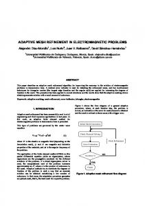
In [10], an algorithm is devised to solve a system of nonlinear equations, L(u) = f . Starting on a coarse grid, given an initial guess, the system is linearized and the linearized FOSLS functional is then minimized on a finite element space. At this point, several AMG V-cycles are performed until there is little to gain in accuracy-per-computational-cost. The system is then relinearized and the minimum of the new linearized FOSLS functional is searched for in the same manner. After each set of linear solves, the relative difference between the computed linearized functional and the nonlinear functional is checked. If they are close and near the minimum of the linearized functional, then it is concluded that we are close enough to the minimum of the nonlinear functional and, hence, we have a good approximation to the solution on the given grid. Next, the approximation is interpolated to a finer grid and the problem is solved on that grid. This process is repeated until an acceptable error has been reached, or until we have run out of computational resources, such as memory. If, as in the case of the MHD equations, it is a time-dependent problem, the whole process is performed at each time step. This algorithm is summarized in the flow chart, figure 1. 3.1
Adaptive Refinement
In the nested iteration algorithm, we decide when to stay on a current mesh and iterate further or interpolate to a finer grid. In [10], it was assumed that the grid is uniformly refined. In other words, it was assumed that there are 2d more points on the next grid than the one before, where d is the dimension of the problem. This is generally not the case when the grids are refined
4
Adler, Manteuffel, McCormick, Nolting, Ruge, and Tang
Fig. 1. Flow chart of nested iteration algorithm.
locally. On a given mesh, after enough Newton steps and linear iterations have been performed, the nonlinear functional is calculated in each element. This indicates in which region of the domain the functional and, hence, the error is large compared to the rest of the domain. Then, the best use of new degrees of freedom is to concentrate them where the error is large. Since the goal of the algorithm is to increase the accuracy-per-computational-cost, we do not want to over solve in areas where the error is already small. The adaptive scheme that we describe here is an efficiency based refinement method, called ACE, that was developed in [12–14]. This scheme estimates both the reduction in the functional and the computational cost that would result from any given refinement pattern. These estimates are used to establish a refinement pattern that attempts to optimize the Accuracy-per-Computational cost (Efficiency), which gives rise to the acronym ACE. The square of the functional value on each element, ǫi , is computed and is ordered such that the local functional value is decreasing: ǫ1 ≥ ǫ2 ≥ . . . ≥ ǫN l ,
(17)
where Nl is the total number of elements on level l. Next, we predict the reduction of the squared functional and the estimated computational work that would result if we were to refine a given percentage of the elements with the most error. Denote the percentage by r ∈ (0, 1] and the number of elements to be refined by r ∗ Nl . Define f (r) to be the squared functional value in the r ∗ Nl elements with largest error, that is, P i