An efficient ILS heuristic for the Vehicle Routing Problem ... - CiteSeerX

An efficient ILS heuristic for the Vehicle Routing Problem with Simultaneous Pickup and Delivery Anand Subramanian, Luiz Satoru Ochi Instituto de Computac¸a˜ o Universidade Federal Fluminense {anand, satoru}@ic.uff.br

Luc´ıdio dos Anjos Formiga Cabral Departamento de Inform´atica Universidade Federal da Para´ıba [email protected]

Technical Report – RT 07/08 Instituto de Computac¸a˜ o – UFF

Abstract This paper deals with the Vehicle Routing Problem with Simultaneous Pickup and Delivery (VRPSPD). A procedure based on the Iterated Local Search (ILS) metaheuristic that uses the Variable Neighborhood Descent (VND) method for performing the local search is proposed. According to literature, the most successful algorithms for the VRPSPD are pure or hybrid versions of the Tabu Search metaheuristic. Our objective here is to show that the ILS can also produce highly competitive results. The algorithm developed was tested on benchmark problems available in the VRPSPD literature and it was found capable of improving several of the known solutions.

1. Introduction The Vehicle Routing Problem (VRP) is a well-known combinatorial optimization problem proposed in the late 1950’s and it is still one of the most studied in the field of Operations Research. The great interest in the VRP is due to its practical importance as well as the high level of difficulty in solving it. Recognized as NP-hard, the VRP with Pickup and Delivery (VRPPD), i.e., the problem where objects or people should be collected and distributed, constitutes an important class of the VRP [3]. The most VRPPD variants studied in the literature are: VRP with Backhauls, VRP with mixed Pickup and Delivery; Dial-a-ride Problem; and the VRP with Simultaneous Pickup and Delivery (VRPSPD). In this work, our interest lies in the VRPSPD, which can be described as follows. Let G = (V, E) be a complete and directed graph with a set of vertices V = 0, ..., n, where the vertex 0 represents the depot (V0 = {0}) and the remaining ones the clients. Each edge (i, j) ∈ E has a non-negative cost ci j satisfying the triangular inequality. Each client i ∈ V −V0 has a demand qi ∈ D for delivery and pi ∈ P for pickup, 1

Instituto de Computac¸a˜ o – UFF

Technical Report RT–07/08

where D and P are the sets containing the amount of a certain cargo (or people) to be distributed and collected respectively. Let C = 1, ..., m be the set of available vehicles with capacity Q . The VRPSPD consists in constructing a set up to m routes with the following requisites: (i) all the pickup and delivery demands should be accomplished; (ii) the capacity of the vehicle should not be exceeded; (iii) only one vehicle can visit a determined client; (iv) the sum of costs should be minimized. A number of applications of the VRPSPD can be found in the beverage industry, where filled bottles are delivered while the empty ones are collected; in grocery stores, where pallets or containers are collected for re-use in merchandise transportation, etc. On the other hand, some clients can demand that the delivery and pickup services should performed at the same time, since, if it is carried out separately, it may imply in additional costs and operational efforts for these customers. Thus, one should consider not only the Distribution Logistics, but also the management of the reverse flow. It is in this context, that the concept of Reverse Logistics arises, which can be defined as the process of planning, implementing and controlling the return of raw materials, inventories under process, finished products and information related to the point of consumption until the point of origin. Therefore, the Distribution Logistic and Reverse Logistic should act together with an aim to guarantee the synchronization between the pickup and delivery operations, as well as their impact on the company’s supply chain, resulting in the customer’s satisfaction and minimization of the operational efforts. According to literature, the most successful algorithms for the VRPSPD are pure or hybrid versions of the Tabu Search metaheuristic. Our objective here is to show that the ILS can also produce highly competitive results. The algorithm proposed in this paper consists of an extension of the ILS heuristic developed in [23] for the VRPSPD with time limits to accomplish a route. Two new perturbation mechanisms are incorporated into this procedure. This paper is organized as follows. Section 2 lists some works related to the VRPSPD. Section 3 deals with the proposed algorithm, describing the constructive and local search procedures, as well as the perturbation mechanisms adopted. Section 4 contains the results obtained and a comparison with the ones found in the literature. Section 5 presents the concluding remarks of this work. 2. Related Works The VRPSPD was first treated in [15], where the author dealt with a case study carried over in public library’s distribution system. The procedure utilized to solve this problem involved the following stages: (i) clients are first clustered in such a way that the vehicle capacity is not exceeded in each group; (ii) one vehicle is assigned to every cluster (iii) Traveling Salesman Problem (TSP) is solved for each group of clients. The cluster-first-route-second approach was applied in [12], in which the routes are clustered by solving an assignment problem and then improved by applying a 3-opt procedure. Some insertion-based heuristics, also capable of solving the problem with, multi-depots are suggested in [22]. Two of them are basically greedy heuristics while a third one extends these procedures by adopting a cluster insertion strategy. Recently the same authors have developed another procedure [18] which involves solutions with certain degree of feasibility. In [9] the VRPSPD is treated under various aspects of reverse logistics and the author proposes a constructive heuristic based on the cheapest feasible insertion criterion, radial surcharge, and the residual 2

Instituto de Computac¸a˜ o – UFF

Technical Report RT–07/08

capacity, where the last one is an adaptation of the load-base approach. The author also investigates the relation between the VRPSPD and other VRP variants. Two methods based on Genetics Algorithms were implemented in [24], where the first one is inspired on the Random Key Method while the second one consists in an improvement heuristic that applies Or-opt movements. An Ant Colony based algorithm was developed in [10]. The same is divided in four main steps: (i) first, a candidate list is formed for each customer; (ii) next, a feasible solution is found and initial pheromone trails on each arc is calculated using it; (iii) routes are constructed and the pheromone trails are modified by both local and global pheromone update; (iv) the routes are improved using the 2-opt movement. In [21] a Large Neighborhood Heuristic (LNS) associated with a procedure similar to the VNS metaheuristic is developed. The authors also solved several variants of the VRPPD. The Tabu Search (TS) metaheuristic has been widely used to solve the VRPSPD. A hybrid procedure is presented in [7] where TS and Variable Neighborhood Descent (VND) are combined. In [17] it is proposed a TS algorithm involving the following neighborhood structures: reallocation, interchange (swap), crossover and 2-opt. TS was also implemented in [11], for the case where only one vehicle is considered. A local search procedure based on the record-to-record travel approximation and tabu lists was proposed in [6]. In [5] multiple neighborhood structures were employed in a hybrid heuristic that combines the principles of the Simulated Annealing and TS metaheuristics In [4] some constructive and local search heuristics are suggested as well as a TS procedure that uses a variable neighborhood structure, in which the node-exchange-based and arc-exchange-based movements were combined. A constructive procedure based on the sweep algorithm is presented in [25]. The authors also propose a reactive TS with the following neighborhood structures: reallocation of a client (shift), exchanging two clients between two different routes (exchange) and reversing the route direction (reverse). A hybrid algorithm which combines the TS and Guided Local Search metaheuristics is developed in [26]. In [23] an ILS based heuristic for the VRPSDP with time limits is proposed. A VND procedure is used in the local search phase while the Double-Bridge perturbation is applied as a diversification movement. An exact approach based on the branch-and-price technique was utilized in [8]. Two different strategies are used to solve the subpricing problem: (i) exact dynamic programming and (ii) state space relaxation. The authors managed to find the optimum solution for instances up to 40 clients. The same technique is applied in [2], where the authors consider the VRPSPD with time-windows constraints. Table 1 summarizes the VRPSPD related works mentioned in this section, describing their main contributions and/or approaches. It can be seen that the interest in the VRPSPD considerably grew up in the past decade. Among the different approaches proposed, the heuristics are the most used so far. In addition, it is possible to verify that, in the last five years, the metaheuristics are being widely employed in the literature. One the other hand, the exact strategies have not been much explored when compared to the heuristics methods. To the best of our knowledge, the TS based heuristics proposed in [25] and [26] have obtained the best known results in most of the benchmark problems available in the VRPSPD

3

Instituto de Computac¸a˜ o – UFF

Technical Report RT–07/08

literature.

Work

Table 1. VRPSPD related works Year Contributions and/or Approach

Min [15]

1989

First Work Case study in a public library

Halse [12]

1992

Cluster-first, route-second strategy 3-opt procedure

Salhi and Nagy [22]

1999

Insertion based heuristics

Dethloff [9]

2001

Constructive heuristic based on cheapest insertion, radial surcharge and residual capacity

Angelelli and Mansini[2]

2001

Branch-and-price for the VRPSPD with TW

Vural [24]

2002

Genetic Algorithm

Gokc¸e [10]

2003

Ant Colony

Ropke and Pisinger [21]

2004

Large Neighborhood Search

Nagy and Salhi [18]

2005

Heuristics with different levels of feasibility

Crispim and Brandao [7]

2005

TS + VND

Dell’amico et al. [8]

2005

Branch-and-price based on dynamic programming and state space relaxation

Chen and Wu [6]

2006

Record-to-record travel + Tabu Lists

Montan´e and Galv˜ao [17]

2006

TS Algorithm

Gribkovskaia et al. [11]

2006

TS for the VRPSPD with a single vehicle

Bianchessi and Righini [4]

2007

Constructive and Local Search Heuristics TS + VNS

Wassan et al. [25]

2008

Reactive TS

Subramanian and Cabral [23]

2008

ILS Heuristic for the VRPSPD with Time Limit Time Limit

Zachariadis et al. [26]

2009

TS + Guided Local Search

3. Solution Procedure The proposed algorithm (ILS-VND) works as follows. The procedure is executed MaxIter times, where a initial solution is generated by a greedy heuristic and then it is improved by a procedure based on the ILS metaheuristic which realizes a local search by means of a VND heuristic. The pseudocode is described in the Alg. 1, where s∗ corresponds do the best solution, v is the number of vehicles imputed and γ is a parameter treated in details in Subsection 3.1. 3.1 Constructive Procedure

The method employed for building a feasible initial solution involves a greedy approach and is an adaptation of the insertion heuristic developed in [9]. 4

Instituto de Computac¸a˜ o – UFF

Technical Report RT–07/08

Algorithm 1 ILS-VND 1: Procedure ILS-VND(MaxIter, MaxIterILS, γ, v, seed) 2: LoadData( ); 3: f ∗ := ∞; 4: for k :=1,..., MaxIter do 5: s := GenerateInitialSolution(γ, v, seed); 0 6: s := s; 7: iterILS := 0; 8: while iterILS < MaxIterILS do 9: s := VND(N(.), f (.), r, s) {r = n0 of neighborhoods} 0 10: if f (s) < f (s ) then 0 11: s := s; 0 12: f (s ) := f (s); 13: iterILS := 0; 14: end if; 0 15: s := Perturb(s ); 16: iterILS := iterILS + 1; 17: end while; 0 18: if f (s ) < f ∗ then 0 ∗ s := s ; 19: 0 ∗ 20: f := f (s ); 21: end if; 22: end for; 23: return; 24: end ILS-VND. Algorithm 2 GenerateInitialSolution 1: Procedure GenerateInitialSolution(seed, γ, v) / 2: s := 0; 3: Initialize© the Candidate List(CL) ª 4: Let s = s1 , . . . , sv be the set composed by v empty routes; 5: t := 1; 6: while t ≤ v do 7: st := e ∈ CL selected at random; 8: Update CL; 9: t := t + 1; 10: end while; 11: while CL 6= 0/ do 12: Evaluate the value of each cost g(e) for e ∈ CL; 13: gmin := min{g(e)|e ∈ CL}; 14: n := client e associated to gmin ; 15: s := s ∪ {n}; 16: Update CL; 17: end while; 18: return s; 19: end GenerateInitialSolution.

The pseudocode of the constructive procedure is shown in Alg. 2. To begin with, the number of vehicles v to be considered for constructing the initial solution is pre-determined. Then, all routes are filled with a client e, chosen at random from the Candidate List (CL). Later, the clients belonging to the CL are evaluated according to the insertion criterion expressed by the eq. (1). 5

Instituto de Computac¸a˜ o – UFF

Technical Report RT–07/08

¡ ¢ g (ev ) = cik + ck j − ci j − γ (c0k + ck0 )

(1)

The first part of eq. (1) is related to the well-known cheapest feasible insertion criterion, which consists of a greedy approach that takes into account the least additional cost regarding the insertion of the client k between the clients i and j of the route v. Naturally, only the feasible insertions are admitted. The second part corresponds to a surcharge used to avoid late insertions of clients remotely located. The cost from the depot and back is weighted by a factor γ ∈ [0, 1]. The client e associated to gmin is then added to the solution s. The constructive procedure ends when all the clients have been added to the solution s. 3.2 Local Search

The local search phase (Alg. 3) is performed by a heuristic based on the VND algorithm. The variable neighborhood descent method [16] systematically modifies the neighborhood structures that belong to a set N in a deterministic way. In the proposed algorithm, a set of ten neighborhood structures was utilized. Most of them were employed in [5], except for the Reverse movement which was applied in [18] and [25]. Just the feasible movements are admitted, i.e., the ones that do not violate the maximum load constraints. Therefore, every time an improvement occurs, one should check whether this new solution is feasible or not. Among the ten neighborhoods adopted here in a exhaustive fashion, six perform movements between different routes and four inside the routes. The N set of neighborhoods (between the routes) is described next. The other four are presented later in this Subsection. Shift(1,0) – N (1) – A client c is transferred from a route r1 to a route r2 . The vehicle load is checked as follows. All clients located before the insertion’s position have their loads added by qc (delivery demand of the client c), while the ones located after have their loads added by pc (pick-up demand of the client c). It is worth mentioning that certain devices to avoid unnecessary infeasible movements can be employed. For instance, before checking the insertion of c in some certain route, a preliminary verification is performed in r2 to evaluate the vehicle load before leaving, ∑i∈r2 qi + qc , and when arriving, ∑i∈r2 pi + pc , the depot. If the load exceeds the vehicle capacity Q, then all the remaining possibilities of inserting c in this route will be always violated. Crossover – N (2) – The arc between adjacent clients c1 and c2 , belonging to a route r1 , and the one between c3 and c4 , from a route r2 , are both removed. Later, an arc is inserted connecting c1 and c4 and another is inserted linking c3 and c2 . The procedure for testing the vehicle load is more complex in comparison to Shift(1,0). At first, the initial (l0 ) and final (l f ) vehicle loads of both routes are calculated. If the values of l0 and l f do not exceed the vehicle capacity Q then the remaining loads are verified through the following expression: li = li−1 + pi − qi . Hence, if li surpasses Q, the movement is infeasible. Swap(1,1) – N (3) – Permutation between a client c1 from a route r1 and a client c2 , from a route r2 . The loads of the vehicles of both routes are examined in the same manner. For example, in case of r2 , all clients situated before the position that c2 was found (now replaced by c1 ), have their values added by qc1 and subtracted by qc2 , while the load of the clients positioned after c1 increases by pc1 and decreases by pc2 . 6

Instituto de Computac¸a˜ o – UFF

Technical Report RT–07/08

Shift(2,0) – N (4) – Two consecutive clients, c1 and c2 , are transferred from a route r1 to a route r2 . The vehicle load is tested as in Shift(1,0). Swap(2,1) – N (5) – Permutation of two consecutive clients, c1 and c2 , from a route r1 by a client c3 from a route r2 . The load is verified by means of an extension of the approach used in the neighborhoods Shift(1,0) and Swap(1,1). Swap(2,2) – N (6) – Permutation between two consecutive clients, c1 and c2 , from a route r1 by another two consecutive c3 and c4 , belonging to a route r2 . The load is checked just as Swap(1,1). Algorithm 3 VND 1: Procedure VND(N(.), f (.), r, s) 2: {Let r be the number of neighborhoods structures} 3: k := 1; {current neighborhood} 4: while k ≤ r do 0 5: Find the best neighbor s of s ∈ N k ; 0 6: if f (s ) < f (s) then 0 s := s ; 7: 0 8: f (s) := f (s ); 9: k := 1; 10: {intensification in the modified routes} 0 s := Or-opt(s); 11: 00 0 12: s := 2-opt(s ); 000 00 13: s := Exchange(s ); 0000 000 14: s := Reverse(s ); 0000 15: if f (s ) ≤ f (s) then 0000 16: s := s ; 0000 17: f (s) := f (s ); 18: end if; 19: else 20: k := k + 1; 21: end if; 22: end while; 23: return s; 24: end VND.

In case of improvement of the current solution, one should aim to further refine the quality of the routes that contributed to reduce the objective function, that is, those which participated in the last betterment move. Hence, the following different neighborhoods are explored: Or-opt – Introduced in [19] for the TSP, where one, two or three consecutive clients are removed and inserted in another position of the route. 2-opt – Two nonadjacent arcs are removed and another two are added to form a new route. Exchange – Permutation between two clients. Reverse – This movement reverses the route direction if the value of the maximum load of the corresponding route is reduced.

7

Instituto de Computac¸a˜ o – UFF

Technical Report RT–07/08

3.3 Perturbation Mechanism

A set P of three perturbation mechanisms were adopted. Whenever the Perturb() function is called, one of the movements described below is randomly selected. Ejection Chain – P(1) – Applied in [20] for the classical version of the VRP, this movement was employed here as perturbation mechanism and it works as follows. A client from a route r1 is transferred to a route r2 , next, a client from r2 is transferred to a route r3 and so on. The movement ends when one client from the last route rv is transferred to r1 . The clients are chosen at random and the movement is applied only when there are up to 12 routes. It has been noticed that the application of the Ejection Chain, in most cases, had no effect when there are more than 12 routes. Double-Swap – P(2) – Two Swap(1,1) movements are performed in sequence randomly. Double-Bridge – P(3) – Introduced in [14], this perturbation was originally developed for the TSP and consists in cutting four edges of a given route and inserting another four. In our case, the double-bridge movement is randomly applied in all routes. When there are a large number of routes this perturbation is applied in just some of them. This prevents exaggerated perturbations which may lead to unpromising regions of the solution space. As stated in [13], several applications of the ILS for the TSP have employed this type of perturbation, and it has been noted to be effective for different instance sizes. 4. Computational Results The proposed algorithm, ILS-VND, was coded in C++ programming language and executed in a PC Intel Core 2 Quad 2.50 GHz with 3.2 GB of RAM memory and operating system Ubuntu Linux 8.04 (kernel 2.6.24-17). The procedure was tested in benchmark problems found in the literature related to the VRPSPD. A comparison was made with the best known results. The number of iterations (MaxIter) and perturbations allowed (MaxIterILS), was 15 and 30 respectively. They were calibrated empirically after preliminary tests with different values. Thirty executions were performed for each one of the different parameterizations of γ. In the instances proposed in [9] and [17] the value of γ varied in the interval [0, 1] with increment of 0.10, while in the instances proposed in [22] the value was varied in the interval [0, 0.5] with increment of 0.05. The results found by the ILS-VND in the instances generated in [9] are shown in Table 2, where n is the number of clients; vi represents the number of vehicles initially imputed; v f corresponds to the number of vehicles of the final solution; Best Sol. indicates the best solution found by the ILS-VND; t is the execution time related to the run where the Best Sol. was found; Avg. Sol. represents the average solution obtained by the ILS-VND associated with the value of γ in which the Best Sol. was determined; Avg. t corresponds to the average execution runtime; and Gap is the deviation of the Avg. Sol with respect to the Best Sol. Table 3 shows a comparison between the solutions obtained by the ILS-VND and the best ones reported in the literature (as per our knowledge), namely those found in [21] and [26]. From Table 2 it is possible to affirm that the ILS-VND demonstrated a consistent performance, since the average gap between the best solutions and the average solutions was only 0.14% with the highest value in the instances SCA3-7 and SCA8-7. It can be observed from Table 3 that among the 40 instances, the ILS-VND has improved the results of 5 instances and equaled another 35, with an average gap of 8

Instituto de Computac¸a˜ o – UFF

Technical Report RT–07/08

Table 2. Results obtained in Dethloff’s instances Problem

n

vi

vf

Best Sol.

t∗

Avg. Sol.

SCA3-0

50

5

4

635.62

0.90

SCA3-1

50

4

4

697.84

1.12

SCA3-2

50

4

4

659.34

SCA3-3

50

4

4

SCA3-4

50

4

SCA3-5

50

SCA3-6

Avg. t ∗

Gap (%)

γ

637.88

0.36

0.40

0.86

697.84

0.00

0.00

1.32

1.19

659.34

0.00

0.00

1.36

680.04

1.13

680.04

0.00

0.10

1.34

4

690.50

1.32

690.50

0.00

0.00

1.52

4

4

659.90

1.17

659.90

0.00

0.10

1.41

50

4

4

651.09

1.23

651.09

0.00

0.00

1.44

SCA3-7

50

4

4

659.17

1.69

663.93

0.72

1.00

1.82

SCA3-8

50

4

4

719.47

1.08

719.47

0.00

0.00

1.25

SCA3-9

50

4

4

681.00

1.03

681.00

0.00

0.00

1.23

SCA8-0

50

9

9

961.50

2.52

966.13

0.48

0.10

2.90

SCA8-1

50

9

9

1049.65

2.98

1050.70

0,10

0.60

3.38

SCA8-2

50

9

9

1039.64

3.42

1040.70

0.10

0.40

3.86

SCA8-3

50

9

9

983.34

3.44

983.62

0.03

0.80

3.90

SCA8-4

50

9

9

1065.49

2.74

1066.34

0.08

0.90

3.59

SCA8-5

50

9

9

1027.08

3.44

1031.02

0.38

0.70

3.82

SCA8-6

50

9

9

971.82

2.48

972.33

0.05

0.00

3.21

SCA8-7

50

9

9

1051.28

5.34

1058.89

0.72

0.40

5.41

SCA8-8

50

9

9

1071.18

2.05

1071.18

0.00

0.00

2.74

SCA8-9

50

9

9

1060.50

3.10

1062.07

0.15

0.60

3.34

CON3-0

50

4

4

616.52

2.02

617.35

0.13

1.00

2.43

CON3-1

50

4

4

554.47

1.83

554.47

0.00

1.00

2.10

CON3-2

50

4

4

518.00

2.10

519.72

0.33

0.70

1.98

CON3-3

50

4

4

591.19

1.34

591.19

0.00

0.00

1.54

CON3-4

50

4

4

588.79

1.79

589.50

0.12

0.90

2.19

CON3-5

50

4

4

563.70

1.71

563.78

0.01

0.50

2.09

CON3-6

50

4

4

499.05

1.93

500.36

0.26

1.00

2.36

CON3-7

50

4

4

576.48

1.52

577.08

0.10

0.60

1.86

CON3-8

50

4

4

523.05

1.51

523.05

0.00

0.10

1.81

CON3-9

50

4

4

578.24

1.58

580.56

0.40

0.70

2.02

CON8-0

50

9

9

857.17

3.74

857.89

0.08

0.90

4.14

CON8-1

50

9

9

740.85

2.82

740.87

0.00

0.90

3.73

CON8-2

50

9

9

712.89

2.46

713.33

0.06

1.00

2.86

CON8-3

50

10

10

811.07

2.82

811.77

0.09

0.80

3.53

CON8-4

50

9

9

772.25

3.37

772.25

0.00

0.80

4.30

CON8-5

50

9

9

754.88

3.30

756.88

0.26

0.40

3.68

CON8-6

50

9

9

678.92

3.04

681.81

0.43

0.80

3.68

CON8-7

50

9

9

811.96

2.73

812.98

0.13

0.30

3.24

CON8-8

50

9

9

767.53

3.42

768.59

0.14

0.80

3.70

CON8-9

50

9

9

809.00

3.60

809.90

0.11

0.70

4.26

(*) CPU time in seconds in a PC Intel Core 2 Quad 2.5 GHz.

-0.01%. The times presented in Table 3 (and also Tables 5 and 7) give an idea of the computational effort demanded, but since they are referred to machines with distinct configurations, it is not possible to make a direct comparison among the respective algorithms. Table 4 presents the results obtained on the instances generated in [22] and Table 5 shows a comparison between the ILS-VND and the best known results found in the literature, namely those determined 9

Instituto de Computac¸a˜ o – UFF

Technical Report RT–07/08

Table 3. Comparison between ILS-VND and literature results in Dethloff’s instances Problem

Ropke and Pisinger Sol.

v

t∗

Zachariadis et al. Sol.

v

ILS-VND

Gap(%)

t ∗∗ .

Sol.

v

t ∗∗∗

SCA3-0

636.1

-

232

636.06

4

2.83

635.62

4

0.90

-0.08

SCA3-1

697.8

-

170

697.84

4

2.12

697.84

4

1.12

0.00

SCA3-2

659.3

-

160

659.34

4

2.58

659.34

4

1.19

0.00

SCA3-3

680.6

-

182

680.04

4

3.13

680.04

4

1.13

0.00

SCA3-4

690.5

-

160

690.50

4

2.68

690.50

4

1.32

0.00

SCA3-5

659.9

-

178

659.90

4

2.56

659.90

4

1.17

0.00

SCA3-6

651.1

-

171

651,09

4

4.40

651.09

4

1.23

0.00

SCA3-7

666.1

-

162

659.17

4

2.98

659.17

4

1.69

0.00

SCA3-8

719.5

-

157

719.47

4

3.98

719.47

4

1.08

0.00

SCA3-9

681.0

-

167

681.00

4

3.86

681.00

4

1.03

0.00

SCA8-0

975.1

-

98

961.50

9

3.21

961.50

9

2.52

0.00

SCA8-1

1052.4

-

95

1050.20

9

3.55

1049.65

9

2.98

-0.05 0.00

SCA8-2

1039.6

-

83

1039.64

9

4.67

1039.64

9

3.42

SCA8-3

991.1

-

94

983.341

9

3.29

983.34

9

3.44

0.00

SCA8-4

1065.5

-

84

1065.49

9

2.68

1065.49

9

2.74

0.00 0.00

SCA8-5

1027.1

-

96

1027.08

9

4.50

1027.08

9

3.44

SCA8-6

972.5

-

93

971.82

9

2.67

971.82

9

2.48

0.00

SCA8-7

1061.0

-

92

1052.17

9

4.32

1051.28

9

5.39

-0.08

SCA8-8

1071.2

-

85

1071.18

9

3.43

1071.18

9

2.05

0.00

SCA8-9

1060.5

-

86

1060.50

9

4.12

1060.50

9

3.10

0.00

CON3-0

616.5

-

171

616.52

4

3.89

616.52

4

2.02

0.00

CON3-1

554.5

-

190

554.47

4

2.97

554.47

4

1.83

0.00

CON3-2

521.4

-

176

519.26

4

3.32

518.00

4

2.10

-0.24

CON3-3

591.2

-

177

591.19

4

2.78

591.19

4

1.34

0.00

CON3-4

588.8

-

173

589.32

4

3.12

588.79

4

1.79

0.00

CON3-5

563.7

-

179

563.70

4

3.45

563.70

4

1.71

0.00

CON3-6

499.1

-

195

500.80

4

2.98

499.05

4

1.93

0.00

CON3-7

576.5

-

226

576.48

4

2.40

576.48

4

1.52

0.00

CON3-8

523.1

-

174

523.05

4

5.02

523.05

4

1.51

0.00

CON3-9

578.2

-

163

580.05

4

3.14

578.24

4

1.58

0.00

CON8-0

857.2

-

86

857.17

9

3.40

857.17

9

3.74

0.00

CON8-1

740.9

-

81

740.85

9

3.73

740.85

9

2.82

0.00

CON8-2

716.0

-

84

713.14

9

2.87

712.89

9

2.46

-0.04

CON8-3

811.1

-

91

811.07

10

3.82

811.07

10

2.82

0.00

CON8-4

772.3

-

87

772.25

9

2.98

772.25

9

3.37

0.00

CON8-5

755.7

-

94

756.91

9

5.76

754.88

9

3.30

-0.11

CON8-6

693.1

-

96

678.92

9

4.00

678.92

9

3.04

0.00

CON8-7

814.8

-

94

811.96

9

2.46

811.96

9

2.73

0.00

CON8-8

774.0

-

94

767.53

9

4.21

767.53

9

3.42

0.00

CON8-9

809.3

-

92

809.00

9

3.87

809.00

9

3.60

0.00

(*) CPU time in seconds in a PC Pentium IV 1.5 GHz. (**) CPU time in seconds in a PC Pentium IV 2.4 GHz. (***) CPU time in seconds in a PC Intel Core 2 Quad 2.5 GHz.

in [26] and [25]. Analyzing Table 4, it can be verified that the average gap between the best solutions and the average solutions of the ILS-VND was 1.60%, with the highest value in the instance CMT11X. Table 5 shows that among the 14 instances listed, the ILS-VND algorithm was capable of improving the 10

Instituto de Computac¸a˜ o – UFF

Technical Report RT–07/08

Table 4. Results obtained in Salhi and Nagy’s instances Problem

n

vi

vf

Best Sol.

t∗

Avg. Sol.

CMT1X

50

3

3

466.77

1.10

CMT1Y

50

3

3

466.77

1.08

CMT2X

75

6

6

684.21

CMT2Y

75

6

6

CMT3X

100

5

CMT3Y

100

CMT12X

100

CMT12Y

Avg. t ∗

Gap (%)

γ

467.61

0.16

0.30

1.64

467.00

0.07

0.35

1.42

6.99

689.57

0.70

0.35

7.07

684.21

5.84

686.74

0.37

0.10

5.57

5

721.40

7.77

726.17

0.66

0.50

6.80

5

5

721.40

6.40

726.32

0.68

0.50

7.37

6

5

662.22

8.02

673.91

1.74

0.05

7.28

100

6

5

662.22

6.05

673.12

1.46

0.10

7.32

CMT11X

120

5

4

839.39

12.58

879.36

4.55

0.45

14.51

CMT11Y

120

5

4

841.88

14.80

878.68

4.19

0.45

14.99

CMT4X

150

7

7

852.83

50.72

866.28

1.55

0.40

48.99

CMT4Y

150

7

7

852.46

46.06

864.41

1.38

0.45

49.10

CMT5X

199

11

10

1030.55

53.51

1054.29

2.25

0.15

49.20

CMT5Y

199

11

10

1031.17

58.74

1059.83

2.70

0.30

54.00

(*) CPU time in seconds in a PC Intel Core 2 Quad 2.5 GHz.

Table 5. Comparison between ILS-VND and literature results in Salhi and Nagy’s instances Problem

Wassan et al. Sol.

v

Zachariadis et al. t∗

Sol.

v

ILS-VND

Gap(%)

t ∗∗

Sol.

v

t ∗∗∗

CMT1X

468.30

3

48

469.80

3

2.89

466.77

4

1.10

-0.33

CMT1Y

458.96

3

69

469.80

3

3.85

466.77

4

1.08

1.68

CMT2X

668.77

6

94

684.21

6

7.42

684.21

6

6.99

2.31

CMT2Y

663.25

6

102

684.21

6

8.02

684.21

6

5.84

3.16

CMT3X

729.63

5

294

721.27

5

11.62

721.40

5

6.80

0.02

CMT3Y

745.46

5

285

721.27

5

13.53

721.40

5

7.37

0.02

CMT12X

644.70

5

242

662.22

5

11.80

662.22

5

8.02

2.71

CMT12Y

659.52

6

254

662.22

5

7.59

662.22

5

7.32

0.41 0.09

CMT11X

861.97

4

504

838.66

4

17.78

839.39

4

12.58

CMT11Y

830.39

4

325

837.08

4

14.26

841.88

4

14.80

1.38

CMT4X

876.50

7

558

852.46

7

27.75

852.83

7

50.72

0.04

CMT4Y

870.44

7

405

852.46(1)

7

31.20

852.46

7

46.06

0.06(2)

CMT5X

1044.51

9

483

1030.55

10

51.67

1030.55

10

53.51

0.00

CMT5Y

1054.46

9

533

1030.55

10

58.81

1031.17

10

58.74

0.06

(1) A better result (852.35) was found in [6]. (2) Gap with respect to the result found in [6]. (*) CPU time in seconds in a Sun-Fire-V440 with a UltraSPARC-IIIi 1062 MHz processor. (**) CPU time in seconds in a PC Pentium IV 2.4 GHz. (***) CPU time in seconds in a PC Intel Core 2 Quad 2.5 GHz.

result of one instance and equaling another one, resulting in an average gap of 0.83% with respect to the best results found in the literature. It is important to emphasize that the gap in the instances CMT3X, CMT3Y, CMT4X, CMT4Y CMT11X and CMT5Y was up to 0.09%. Table 6 presents the results found in the instances proposed in [17], while Table 6 illustrates a comparison between the results determined by ILS-VND and those found in [17] and [26]. From Table 7, it is observed that the average gap between the average solutions and the best solutions was 0.70%, with the highest gap in the instance r1 2 1. When comparing the results found in the literature with the ones

11

Instituto de Computac¸a˜ o – UFF

Technical Report RT–07/08

˜ Table 6. Results obtained in Montane´ and Galvao’s instances n

vi

vf

Best Sol.

t∗

Avg. Sol.

r101

100

12

12

1010.90

10.51

1020.74

0.97

0.20

r201

100

3

3

666.20

6.24

666.39

0.03

0.20

7.10

c101

100

16

16

1220.26

12.73

1222.48

0.18

0.70

10.73

c201

100

5

5

662.07

4.18

662.19

0.02

0.10

4.76

rc101

100

10

10

1059.32

9.48

1063.27

0.37

0.40

11.28

Problem

Gap (%)

γ

Avg. t ∗ 12.74

rc201

100

3

3

672.92

4.21

672.92

0.00

0.60

25.28

r1 2 1

200

23

23

3371.29

95.79

3420.79

1.47

0.60

86.38

r2 2 1

200

5

5

1665.58

24.13

1678.78

0.79

0.20

24.35

c1 2 1

200

29

28

3640.20

95.17

3654.78

0.40

0.90

89.76

c2 2 1

200

10

9

1728.14

41.94

1735.44

0.42

0.40

38.52

rc1 2 1

200

25

23

3327.98

76.30

3364.22

1.09

0.40

83.71

rc2 2 1

200

5

5

1560.00

34.28

1563.65

0.23

1.00

35.03

r1 4 1

400

55

54

9695.77

546.39

9787.71

0.95

0.30

480.51

r2 4 1

400

11

10

3574.86

231.73

3623.95

1.37

1.00

235.71

c1 4 1

400

63

63

11124.68

524.35

11193.29

0.62

1.00

505.96

c2 4 1

400

16

15

3575.63

293.18

3618.43

1.20

0.50

276.70

rc1 4 1

400

53

52

9602.53

550.90

9699.70

1.01

0.30

502.54

rc2 4 1

400

11

11

3416.61

291.15

3468.34

1.51

0.40

266.75

(*) CPU time in seconds in a PC Intel Core 2 Quad 2.5 GHz.

˜ Table 7. Comparison between ILS-VND and literature results in Montane´ and Galvao’s instances Problem

Montan´e and Galv˜ao Sol.

r101 r201 c101 c201 rc101 rc201 r1 2 1

v

1042.62 12 671.03

t∗ 12.20

3

12.02

1259.79 17

12.07

5

12.40

1094.15 11

666.01

12.30

674.46

3

12.07

3447.20 23

55.56

Zachariadis et al.

ILS-VND

Gap(%)

v

t ∗∗

Sol.

v

t ∗∗∗

1019.48 12

10.5

1010.90 12

10.51

Sol. 666.20

3

8.7

1220.99 16

10.2

5

5.7

1059.32 10

662.07

12.9

672.92

666.20

-0.84

3

6.24

0.00

1220.26 16

12.73

-0.06

5

4.18

0.00

1059.32 10

9.48

0.00

3

4.21

0.00

662.07

3

10.5

672.92

3393.31 23

61.8

3371.29 23

95.79

-0.65 -0.48

r2 2 1

1690.67

5

50.95

1673.65

5

47.4

1665.58

5

24.13

c1 2 1

3792.62 29

52.21

3652.76 28

66.3

3640.20 28

95.17

-0.34

c2 2 1

1767.58

65.79

1735.68

60.9

1728.14

41.94

-0.43

rc1 2 1

3427.19 24

58.39

3341.25 23

45.3

3327.98 23

76.30

-0.40

rc2 2 1

1645.94

52.93

1562.34

62.4

1560.00

34.28

-0.15

9 5

9 5

9 5

r1 4 1

10027.81 54 330.42

9758.77 54 315.3

9695.77 54 546.39

-0.65

r2 4 1

3695.26 10 324.44

3606.72 10 273.6

3574.86 10 231.73

-0.88

c1 4 1

11676.27 65 287.12 11207.37 63 283.5 11124.29 63 524.35

-0.74

c2 4 1

3732.00 15 330.20

3630.72 15 336.0

3575.63 15 293.18

-1.52

rc1 4 1

9883.31 52 286.66

9697.65 52 145.8

9602.53 52 550.90

-0.98

rc2 4 1

3603.53 11 328.16

3498.30 11 345.0

3416.61 11 291.15

-2.34

(*) CPU time in seconds in a PC Athlon XP 2.0 GHz. (**) CPU time in seconds in a PC Pentium IV 2.4 GHz. (***) CPU time in seconds in a PC Intel Core 2 Quad 2.5 GHz.

determined by the ILS-VND (Table 7), one can notice that the ILS-VND had improved the results of 14 instances and equaled another 4, leading to an average gap of -0.58%. It is worth mentioning that even 12

Instituto de Computac¸a˜ o – UFF

Technical Report RT–07/08

the average solution obtained by the ILS-VND in the instances c2 2 1, c1 4 1, c2 4 1 and rc2 4 1 was better than the best ones reported by the literature. 1

Probability

0.8

0.6

0.4

0.2

0 20

40

60

80 100 120 Time to target value (s)

140

160

180

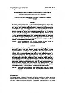
Figure 1. Cumulative probability distribution plot for the time to target solution of the instance r101.

1

Probability

0.8

0.6

0.4

0.2

0 50

100 150 Time to target value (s)

200

250

Figure 2. Cumulative probability distribution plot for the time to target solution of the instance c2 2 1.

13

Instituto de Computac¸a˜ o – UFF

Technical Report RT–07/08

1

Probability

0.8

0.6

0.4

0.2

0 50

100

150 200 250 300 Time to target value (s)

350

400

450

Figure 3. Cumulative probability distribution plot for the time to target solution of the instance rc2 4 1.

An empirical analysis was done in order to illustrate the convergence behavior of the ILS-VND algorithm. In all the cases the value of the best known solution found in the literature was chosen as the target value (stopping criterion). The method employed to plot the empirical distribution for the time to target solution follows the one described in [1]. A probability pi = (i − 1/2)/n is associated with the i-th sorted running time ti and n points zi = (ti , pi ) are plotted, where n is the number of executions, which in our case was n = 100. From Fig. 1 it can be observed that in 80% of the executions the time to target solution was up to 60 seconds. The graph displayed in Fig. 2 shows that for about 80% of the runs the time to find the target solution was up to 125 seconds. In Fig. 3 one can verify that in about 90% of the cases the target was found in less than 225 seconds. These results are encouraging, particularly in the largest instances, since it illustrates, along with the results shown in Table 6, that the proposed algorithm systematically produces good quality solutions in an acceptable time. 5. Concluding Remarks This paper dealt with the Vehicle Routing Problem with Simultaneous Pickup and Delivery. In order to solve it, a hybrid algorithm based on the Iterated Local Search metaheuristic, which uses a VND procedure in the local search phase, was proposed. It is an extension of the heuristic developed in [23] for the VRPSPD with lime limits in which two new perturbation mechanisms were added, specifically, Ejection Chain and Double Swap. The algorithm developed was tested in 72 instances reported in the literature and it was found capable of improving the result of 20 instances and had equaled the solution of another 41. In the 40 instances 14

Instituto de Computac¸a˜ o – UFF

Technical Report RT–07/08

generated in [9], the ILS-VND improved the results of 5 instances and equaled 35, with an average gap of -0.01% with respect to the best results indicated in the literature. In the 14 instances formulated in [22], one result was improved, while another one equaled the best known solution. In addition, the gap in another 5 cases was up to 0.09%. In the 18 instances proposed by [17], the ILS-VND improved the solution of 14 instances and equaled another 4, with an average gap of -0.58%. The main characteristic of these test-problems is the fact of having some instances with more clients than the other ones proposed in [9] and [22]. Hence, the empirical results obtained are very promising since it shows the efficiency of the proposed algorithm in solving instances with higher dimensions. Finally, for future work, one can suggest: (i) incorporating more efficient procedures to reduce the dependence of the factor γ for generating the initial solution, (ii) searching for alternatives to reduce the computational effort in some neighborhoods in such a way that the local search performance is not compromised, (iii) implementing other perturbation mechanisms, (iv) performing hybridizations, (v) combining exact and heuristic methods and (vi) developing parallel strategies for the proposed algorithm. References [1] R. M. Aiex, M. G. C. Resende, and C. C. Ribeiro. Probability distribution of solution time in GRASP: An experimental investigation. Journal of Heuristics, 8:343–373, 2002. [2] E. Angelelli and R. Mansini. Quantitative Approaches to Distribution Logistics and Supply Chain Management, chapter A branch-and-price algorithm for a simultaneous pick-up and delivery problem, pages 249–267. Springer, Berlin-Heidelberg, 2002. [3] G. Berbeglia, J.-F. Cordeau, I. Gribkovskaia, and G. Laporte. Static pickup and delivery problems: a classification scheme and survey. Top, 15:1–31, April 2007. [4] N. Bianchessi and G. Righini. Heuristic algorithms for the vehicle routing problem with simultaneous pick-up and delivery. Computers & Operations Research, 34(2):578–594, 2007. [5] J. F. Chen. Approaches for the vehicle routing problem with simultaneous deliveries and pickups. Journal of the Chinese Institute of Industrial Engineers, 23(2):141–150, 2006. [6] J. F. Chen and T. H. Wu. Vehicle routing problem with simultaneous deliveries and pickups. Journal of the Operational Research Society, 57(5):579–587, 2005. [7] J. Crispim and J. Brandao. Metaheuristics applied to mixed and simultaneous extensions of vehicle routing problems with backhauls. Journal of the Operational Research Society, 56(7):1296–1302, 2005. [8] M. Dell’Amico, G. Righini, and M. Salanim. A branch-and-price approach to the vehicle routing problem with simultaneous distribution and collection. Transportation Science, 40(2):235–247, 2006. [9] J. Dethloff. Vehicle routing and reverse logistics: the vehicle routing problem with simultaneous delivery and pick-up. OR Spektrum, 23:79–96, 2001. [10] E. I. G¨okc¸e. A revised ant colony system approach to vehicle routing problems. Master’s thesis, Graduate School of Engineering and Natural Sciences, Sabanci University, 2004.

15

Instituto de Computac¸a˜ o – UFF

Technical Report RT–07/08

[11] I. Gribkovskaia, Ø. Halskau, G. Laporte, and M. Vlcek. General solutions to the single vehicle routing problem with pickups and deliveries. European Journal of Operational Research, 180:568– 584, 2007. [12] K. Halse. Modeling and solving complex vehicle routing problems. PhD thesis, Institute of Mathematical Statistics and Operations Research, Technical University of Denmark, Denmark, 1992. [13] H. R. Lourenc¸o, O. C. Martin, and T. St¨utzle. Handbook of Metaheuristics, chapter Iterated Local Search, pages 321–353. Kluwer Academic Publishers, Norwell, MA, 2002. [14] O. Martin, S. W. Otto, and E. W. Felten. Large-step markov chains for the traveling salesman problem. Complex Systems, 5:299–326, 1991. [15] H. Min. The multiple vehicle routing problem with simultaneous delivery and pick-up points. Transportation Research, 23(5):377–386, 1989. [16] N. Mladenovi´c and P. Hansen. Variable neighborhood search. Computers & Operations Research, 24(11):1097–1100, 1997. [17] F. A. T. Montan´e and R. D. Galv˜ao. A tabu search algorithm for the vehicle routing problem with simultaneous pick-up and delivery service. European Journal of Operational Research, 33(3):595– 619, 2006. [18] G. Nagy and S. Salhi. Heuristic algorithms for single and multiple depot vehicle routing problems with pickups and deliveries. European Journal of Operational Research, 162:126–141, 2005. [19] I. Or. Traveling salesman-type combinational problems and their relation to the logistics of blood banking. PhD thesis, Northwestern University, USA, 1976. [20] C. Rego and C. Roucairol. Meta-heuristics Theory and Applications, chapter A Parallel Tabu Search Algorithm Using Ejection Chains for the Vehicle Routing Problem, pages 253–295. Kluwer, Dordrecht, 1996. [21] S. R¨opke and D. Pisinger. A unified heuristic for a large class of vehicle routing problems with backhauls. Technical Report 2004/14, University of Copenhagen, 2004. [22] S. Salhi and G. Nagy. A cluster insertion heuristic for single and multiple depot vehicle routing problems with backhauling. Journal of the Operational Research Society, 50:1034–1042, 1999. [23] A. Subramanian and L. A. F. Cabral. An ILS based heuristic for the vehicle routing problem with simultaneous pickup and delivery. Proceedings of the Eighth European Conference on Evolutionary Computation in Combinatorial Optimisation, Lecture Notes in Computer Science, 4972:135–146, 2008. [24] A. V. Vural. A GA based meta-heuristic for capacited vehicle routing problem with simultaneous pick-up and deliveries. Master’s thesis, Graduate School of Engineering and Natural Sciences, Sabanci University, 2003. [25] N. A. Wassan, A. H. Wassan, and G. Nagy. A reactive tabu search algorithm for the vehicle routing problem with simultaneous pickups and deliveries. Journal of Combinatorial Optimization, 15(4):368–386, 2008.

16

Instituto de Computac¸a˜ o – UFF

Technical Report RT–07/08

[26] E. E. Zachariadis, C. D. Tarantilis, and C. T. Kiranoudis. A hybrid metaheuristic algorithm for the vehicle routing problem with simultaneous delivery and pick-up service. Expert Systems with Applications, 36(2):1070–1081, 2009.

17