An Efficient Multipolling Mechanism for IEEE 802.11 Wireless LANs Shou-Chih Log∗ Guanling Leegg Wen-Tsuen Cheng g
gg
Department of Computer Science, National Tsing Hua University, Taiwan Department of Computer Science and Information Engineering, National Dong Hwa University, Taiwan
Email:
[email protected]
ABSTRACT To expand the support for applications with QoS requirements in Wireless Local Area Networks (WLANs), the 802.11E task group was formed to enhance the current IEEE 802.11 Medium Access Control (MAC) protocol. The multipolling mechanism was discussed in the task group, but some problems remain unsolved. In this paper, we show a novel design of the multipolling mechanism with the advantages of high channel utilization and low implementation overhead. In our proposed mechanism, wireless stations use a priority-based contention scheme to coordinate in themselves the transmission order on the channel. Moreover, we propose a polling schedule mechanism for our proposed multipoll to serve real-time traffic with constant and variable bit rates. The bounded delay requirement of the real-time traffic can be satisfied in our scheduling model. We establish an admission test to estimate the system capacity and to determine whether a new connection can be accepted. We study the performance of our proposed mechanism analytically, as well as through simulated experiments. The results show that the proposed mechanism is efficient than the one discussed in the IEEE 802.11E task group. Keyword: Multipolling, Polling Schedule, IEEE 802.11, Wireless LAN, Medium Access Control
1 INTRODUCTION With the increasing use of portable computers, handsets, and wireless networks, the trend on providing wireless data services has emerged [13]. The wireless communication bandwidth has been largely increased with the advances of channel modulation techniques. The transmission of real-time multimedia data in the wireless networks becomes feasible. The support for real-time services particularly with Quality of Service (QoS) guarantees is a challenge in the wireless networks [8]. The Wireless Local Area Network (WLAN) with high speed and low cost access to the Internet is an excellent platform for providing real-time services. IEEE 802.11 [15] is an international WLAN standard, which covers the specification for the Medium Access Control ∗
To whom all correspondence should be sent.
1
(MAC) sub-layer and the Physical (PHY) layer. The 802.11 WLAN can offer broadband data access through 11Mbps IEEE 802.11b and 54Mbps IEEE 802.11a technologies. The 802.11 WLAN consists of Basic Service Sets (BSS), each of which is composed of wireless stations (STA). The WLAN can be configured as an ad hoc network (an independent BSS) or an infrastructure network (composed of an access point and the associated STAs). The channel access for the STAs in a BSS is under the control of a coordination function. The 802.11 MAC protocol provides two coordination functions: Distributed Coordination Function (DCF) and Point Coordination Function (PCF). The DCF is a contention-based access scheme using Carrier Sense Multiple Access with Collision Avoidance (CSMA/CA). The carrier sensing can be performed both at the physical layer and at the MAC sublayer. Priority levels for access to the channel are provided through the use of Interframe Spaces such as SIFS and DIFS. The backoff procedure is used for collision avoidance, where each STA waits for a backoff time (a random time interval in units of slot times) before each frame transmission. The PCF provides contention-free frame transmission in an infrastructure network by using the Point Coordinator (PC), operating at the access point (AP), to determine which STA currently gets the channel access. The DCF and the PCF can coexist by alternating the Contention Period (CP), during which the DCF is performed, and the Contention-Free Period (CFP), during which the PCF is performed. A CFP and a CP are together referred to as a CFP Repetition Interval or a Superframe. The performance analysis of the DCF was studied in [2][3][10]. The performance of DCF degrades in high traffic loads due to serious collisions. The CSMA/CA is not suitable for data traffic at higher channel speeds as explored in [2] due to the large waste on the backoff time. The influence of various sizes of the backoff time on the channel throughput was observed in [19], and the optimal setting of the backoff time was studied in [5]. The service differentiation and fairness issues over the DCF access scheme were discussed in [1][4][23]. A common technique is to adjust the backoff time according to the traffic priority. The PCF based on a polling scheme is suitable for time-bounded real-time traffic. The simple polling schedules for voice traffic and video traffic were presented in [10] and [22], respectively. Some complex polling schedules were proposed in [6][7][9][14][20]. To expand the support for applications with QoS requirements, the IEEE 802.11E task group [16] is proceeding to build the QoS enhancements of the 802.11 MAC. The techniques of providing prioritized and parameterized QoS data deliveries have been discussed in the task group. An enhanced DCF was proposed, where each traffic flow is assigned with a different backoff time whose value decreases with increasing traffic priority, to achieve the prioritized QoS data delivery. To guarantee the bounded delay requirements in the parameterized QoS data delivery, the Hybrid
2
Coordination Function (HCF) was proposed [12]. In the HCF, a STA can be guaranteed to issue the frame transmission even during the CP by using the Contention-Free Burst (CFB). The CFB can be considered a temporary CFP, during which the transmissions of STAs are coordinated by the polling scheme as the PCF. Moreover, the multipolling mechanism (called Contention-Free Multipoll, CF-Multipoll) was proposed [11] to reduce the polling overhead that the traditional PCF suffers from. In the multipoll, the PC can poll more than one STA simultaneously using a single polling frame. In this paper, we consider how to efficiently serve real-time traffic in the IEEE 802.11 WLAN by using the multipolling mechanism. Our primary contributions are as follows. We propose a novel multipolling mechanism which can increase the channel utilization and is robust in the mobile and error-prone environments. The proposed mechanism can be used in the PCF and the HCF. Moreover, we provide a polling schedule to guarantee the bounded delay requirements of real-time flows. The admission control to limit the number of real-time flows that can be served together is presented too. The reminder of this paper is organized as follows. Section II gives a survey of previous work on the polling schemes for serving real-time traffic. Section III describes our proposed multipolling mechanism. In Section IV, we present a polling schedule to efficiently serve real-time traffic. The performance evaluations are shown in Section V. Finally, we present the conclusion in Section VI.
1.1 Acronyms The acronyms that will be frequently used in the paper are listed below: BSS: basic service set CBR: constant bit rate CP: contention period CF-Multipoll: contention-free multipoll CFP: contention-free period CP-Multipoll: contention period multipoll DCF: distributed coordination function DIFS: distributed interframe space HCF: hybrid coordination function NAV: network allocation vector PC: point coordinator PCF: point coordination function
3
PIFS: point interframe space SIFS: short interframe space STA: wireless station TXOP: transmission opportunity VBR: variable bit rate
2 RELATED WORK Real-time traffic is usually associated with QoS requirements like delay and jitter bounds. Using a centralized coordinator to schedule real-time flows can properly meet their QoS requirements. The polling scheme is a common technique to schedule the transmissions of real-time flows. In the IEEE 802.11 WLAN, the PC maintains a polling list and polls each STA by sending a polling frame (CF-Poll frame) according to the polling list during the CFP. The polling scheme used in the IEEE 802.11 has some limitations [17]: low channel throughput due to the overhead of polling frames, possible repeated collisions if multiple PCs are operating on the same channel in overlapping physical space, and difficulty of correlating the polling rate with the real-time packet arrival rate. To reduce the overhead of polling frames, the multipolling mechanism was discussed in the 802.11E task group. The PC can poll a polling group, which is composed of several flows from different STAs, at a time. Each flow in the same polling group will initiate its own transmission in order (polling order) after receiving the multipolling frame. The polling order in the CF-Multipoll presented in the proposal [11] is specified in the time domain. That is, an individual time interval is assigned to each flow in the polling group. However, this specification method is unpractical. Once a polled STA fails to receive the multipolling frame due to channel errors or move into one other BSS, the time interval allocated to this STA becomes wasted. Also, a polled STA may not fully utilize the allocated time interval when there are not enough data to be transferred. To reduce the failures in receiving the polling frames, the SuperPoll using replicated polling frames was proposed in [14]. In this approach, each polled STA will attach a polling frame to the current transmitted data frame, and the polling frame contains the polling messages of the remaining polled STAs. Clearly, a latter STA in the polling group gets the more probability to receive its polling message. However, the redundant polling frames occupy more channel space. In this paper, we will propose a new multipolling mechanism which can overcome the above problems. To serve constant bit rate (CBR) and variable bit rate (VBR) traffic by the polling scheme, the schedule of polling frames is an important task. A deadline-driven schedule based on a smooth
4
traffic model, where the number of packets that can be arrived in a certain time interval is limited, was proposed in [9]. The PC sends polling frames at appropriate points of time for satisfying the delay requirements of traffic flows. In [6], a STA with real-time traffic will be polled once during each CFP. The polled STA will be allocated with an enough period of time to transmit its data frames. The length of the time is determined by the traffic specification and the maximum delay requirement. However, the length of the time may be over allocated. In [20], STAs are separated into two groups: active group and idle group according to whether there are any pending data ready to be sent. A STA in the active group and a STA in the idle group can simultaneously respond to the polling from the PC by using signals of different strengths. However, this approach does not work well in overlapping BSSes.
3 CONTENTION-BASED MULTIPOLLING MECHANISM In the PCF or the HCF, each STA in the polling list takes a polling frame when polled. This polling scheme is called SinglePoll throughout the paper. Clearly, the number of polling frames for a polling list can be reduced if a multipolling mechanism is used. Here, we propose an efficient multipolling mechanism that has the advantages of high channel utilization and low implementation overhead. Our proposed multipolling mechanism called Contention Period Multipoll (CP-Multipoll) incorporates the DCF access scheme into the polling scheme. Immediate access when medium is idle >= DIFS DIFS
DIFS PIFS SIFS
Busy Medium Defer Access
Backoff Time
Next Frame
Slot time Decrement backoff as long as medium is idle for a slot time
Fig. 1. Basic access method in the DCF.
3.1 DCF Access Scheme At first, we introduce the basic DCF access scheme. Some of the introduced concepts will be used later. In the DCF, any contending STA for the channel will select a backoff time in units of slot times and execute the backoff procedure as follows. If the channel is sensed idle for a DIFS period, a STA starts the transmission immediately. Otherwise, a STA should defer until the channel becomes idle for a DIFS period and then the backoff time is decreased. If the channel is idle for a slot time, a STA decreases the backoff time by one, else freezes the backoff time. When the backoff time becomes zero, a STA begins the frame transmission. If a collision occurs, the STA duplicates the backoff time used in the last transmission and executes the backoff procedure
5
again. This access scheme is outlined in Fig. 1. In the DCF, the virtual carrier sensing by using the Network Allocation Vector (NAV) is performed at the MAC sub-layer. The information on the duration of a frame exchange sequence for one STA is included in the frame header (duration field) and is announced to other STAs. Other contending STAs will wait for the completion of the current frame exchange by updating their NAVs according to the announced duration information. Fig. 2 shows the scenario where the RTS (Request To Send) and CTS (Clear To Send) frames are exchanged before the data frame transmission. Other STAs defer their channel access by setting their NAVs according to the duration field in the RTS, the CTS, or the data frame. The exchange of RTS/CTS frames can also avoid the hidden terminal problem [10]. DIFS
Source
RTS
Data SIFS
Destination Other
SIFS
SIFS
ACK
CTS
NAV(RTS) NAV(CTS)
DIFS
NAV(Data)
Defer Access
Backoff After Defer
Fig. 2. RTS/CTS and NAV Setting.
3.2 Basic Idea The basic idea of CP-Multipoll is to transform the polling order into the contending order which indicates the order of winning the channel contention. We assign different backoff time values to the flows in the polling group and let the corresponding STAs execute the backoff procedures after receiving the CP-Multipoll frame. The contending order of these STAs is the same as the ascending order of the assigned backoff time values. Therefore, to maintain the polling order in a polling group, we can assign the backoff time value incrementally according to the expected polling order. The CP-Multipoll has the following advantages: a polled STA can hold the channel access flexibly depending on the size of local buffered data, so it becomes easy to deal with the data burst; if a polled STA makes no response to the CP-Multipoll, other STAs in the same polling group will detect the channel idle right away and advance the starting of channel contention. Therefore, the CP-Multipoll can decrease the waste of channel space and can afford any polling error. We have to take the following issues into account when the backoff procedure is incorporated into the CP-Multipoll:
6
1. The channel contention during the CP-Multipoll should be protected from the interference of other STAs, which are performing the backoff procedures in the DCF mode, in the neighboring BSSes. 2. The repeated collisions may occur if multiple PCs are performing the CP-Multiple and operating on the same channel in the overlapping space. For example, each of two neighboring STAs simultaneously receives a CP-Multipoll frame with the same backoff time assignment from a different PC. 3. There might exist internal collisions among polled STAs if two polled STAs cannot listen to the transmission each other in the BSS. We provide the following solutions for the above problems: z
As mentioned before, the backoff procedure in the DCF starts the decrement of backoff time after the channel is detected idle for a DIFS period. To deal with the first problem, we make the backoff procedure to be immediately executed in the CP-Multipoll without any deferment. We call it the restricted backoff procedure. The STAs executing the normal backoff procedures after a DIFS period have the less chance to win the channel contention than the STAs executing the restricted ones.
z
For the second problem, we avoid assigning the same backoff time values in the CP-Multipoll among neighboring BSSes if possible. We provide a randomized algorithm to assign the backoff time as introduced in the next subsection.
z
We use the NAV mechanism introduced before to solve the third problem. When a polled STA gets the channel access, the RTS/CTS frames are exchanged between the STA and the PC. The duration information carried in these frames can reserve the channel usage. PC
CP-Multipoll(A, B, C, D)
CP-Multipoll(A) (-2)
(-2)
(-1)
STA A STA B STA C STA D
CP-Multipoll(C)
A's frames
B's frames (-2)
C's RTS
(-3)
C's frames
collision D's frames
(-2)
(-2)
frame transmission
backoff decrement
defer access
Fig. 3. An example of CP-Multipoll.
3.3 A Scenario Example with Error Recovery We explain how the CP-Multipoll works and how the polling errors are recovered using the
7
example shown in Fig. 3. Assume four STAs A, B, C, and D are polled together using the CP-Multipoll. The backoff time values of these four STAs are assumed 1, 2, 3, and 4, respectively. All these four STAs will perform the restricted backoff procedures simultaneously after receiving the CP-Multipoll frame. To confirm that the PC can take the right of channel access back after sending the CP-Multipoll frame, the PC also performs the restricted backoff procedure with backoff time 5. Assume STA A fails to receive the CP-Multipoll frame. This polling error makes no impact on other STAs. When STA B wins the channel contention, RTS/CTS frames with proper duration information are exchanged. Assume STA C cannot listen to any other STA’s channel activity and fails to set its NAV. STA C tries to send the RTS frame; meanwhile, STA B transfers its data frames. An internal collision1 occurs in this case. We specify that a polled STA can at most retransmit the RTS frame three times before receiving the CTS frame. The failure of the RTS/CTS exchange happens when there is an internal collision or when the channel condition is bad. STA C will stop any further action in this case. To recover this error, we explicitly deal with this STA using another poll after the current CP-Multipoll. Assume STA D can set its NAV properly. STA D defers its frame transmission till STA B’s one. After the PC’s backoff time reaches zero, which indicating the end of the current CP-Multipoll, the PC records the STAs which fail in the previous CP-Multipoll. These STAs (STAs A and C in our example) will be polled individually using the CP-Multipoll with a single member in the polling group. The reason why the individual poll is used for the failed STA is that the STA may be in a bad situation and cannot coordinate its transmission properly with others. Involving these failed STAs in the same polling group may cause further internal collisions. octets: 2 Frame Control
2 Duration / ID
6 BSSID
2 Record Count (0-255)
8×RecordCount
4
Poll Record (8 octets)
FCS
AID
TCID
Backoff
(2 octets)
(2 octets)
(2 octets)
TXOP Limit (2 octets)
Fig. 4. The frame format of the CP-Multipoll frame.
3.4 Access Procedure The PC can specify the Transmission Opportunity (TXOP) for each polled STA to limit the amount of uploaded data frames. The TXOP proposed in the IEEE 802.11E task group is a bounded-duration time interval when a particular STA has the right to initiate transmission on the 1
Another case for the internal collision is when a polled STA in one BSS hears the transmission of a STA in another
BSS. The polled STA may postpone its transmission and then collides with other polled STAs.
8
channel. That is, a polled STA can continue sending data frames including those retransmitted frames due to channel errors till its TXOP ends. The frame format of the CP-Multipoll frame is shown in Fig. 4. Each flow in a polling group has its corresponding poll record. The Record Count field is set to the number of poll records. The Poll Record field specifies which STA and how long a STA can perform the frame transmission. The AID subfield contains an association identifier which identifies a STA in the BSS. The TCID subfield specifies the priority of the flow that the polled STA can serve. The Backoff subfield specifies the backoff time value. The TXOP Limit subfield specifies the maximum duration in which the polled STA can transmit frames. We define a null CP-Multipoll frame as one with Record Count set to 0. The null CP-Multipoll frame can cancel the activities of polled STAs in the previous CP-Multipoll. The tasks performed by the PC and the polled STA during the CP-Multipoll are shown in Fig. 5. The channel state is indicated by CCA (Clear Channel Assessment) as described in the standard [15]. In the environment with overlapping BSSes, the frame collision may occur between neighboring BSSes. To confirm that a STA in the overlapping BSS can receive the polling frame, the PC performs the backoff procedure if the channel is sensed busy. That is, we perform an initial backoff before sending the polling frame. The initial backoff decrement starts when the channel is sensed idle for a PIFS period. This can raise the priority of the PC over other STAs to win the channel contention. The backoff time assignment in the initial backoff is dependent on the number of PCs operating in the overlapping space. Before the PC serves those unsuccessfully polled STAs, it sends a null CP-Multipoll frame to cancel any pending polled STA in the BSS. A STA in the BSS will stop the unfinished actions in the previous CP-Multipoll when receiving a null CP-Multipoll frame. To avoid assigning the same backoff time values in the CP-Multipoll among neighboring BSSes, two approaches can be used. One is to use the Inter Access Point Protocol (IAPP) discussed in the IEEE 802.11F task group [16] to coordinate the backoff time assignment. The other is to use a distributed algorithm as introduced below. Let h denote the number of PCs operating in the overlapping space. If one of these PCs generates a CP-Multipoll frame with n poll records, we generate n distinct random numbers from the interval [1, BTmax], where BTmax denotes the maximum possible backoff time and is equal to h×n. Then we sort such generated numbers in ascending order and make the ith number to be the backoff time (bti) of the STA with polling order i (1 ≤ i ≤ n). To guarantee that the PC can re-get the channel access right, the PC also executes the same backoff procedure with backoff time btn + 1 after sending the CP-Multipoll
9
frame. In an independent BSS (i.e., h = 1), the perfect backoff time assignment is with bt1 = 1 and bti = bti-1 + 1 for i ≥ 2.
No
Polled STA's actions
PC's actions
CP-M ultipoll is received
Perform the initial backoff if CCA(busy)
In the poll records ? (AID field)
1. Set internal backoff time BT 2. Send a CP-M ultipoll frame
Yes 1. Set backoff time BT (Backoff subfield) 2. Set max transmission duration (TXOP Limit subfield) 3. Determine the actual transmission duration
CCA idle
busy 1. Response any RTS with CTS 2. Record successful STAs
Backoff time decrement BT = 0
CCA
idle Backoff time decrement
Send a null CP-M ultipoll frame
busy
Set NAV after receiving a frame
Poll unsuccessful STAs individually End
failed & retry < 3 failed & retry >= 3
BT = 0 Frame transmission
RTS/CTS exchange successful Frame transmission
End
No
Pending data for the designated flow ? (TCID subfield)
Transmit a null data frame
Yes
Transmit a data frame
Yes
TXOP end or no more data ?
No
Return
Fig. 5. Flow chart for the CP-Multipoll.
4 POLLING SCHEDULE FOR REAL-TIME SERVICES To make our multipolling mechanism more practical in the real system, we provide the mechanism of polling schedule on real-time flows. In the polling schedule, we will decide when a flow will be polled and how many packets a flow can upload when served according to its delay requirement and its packet arrival rate. We alternate the CFP and the CP in our system to serve
10
both real-time and non-real-time traffic. In the CFP, the types of data frames: DATA+CF-Poll, DATA+CF-ACK, and DATA+CF-Poll+CF-ACK can piggyback the polling message or/and the acknowledgement message. We will take advantage of these types of data frames to reduce the number of control frames exchanged. We consider three types of traffic: CBR, VBR, and ABR (arbitrary bit rate) traffic to be served in the system. The CBR (e.g., audio stream) and VBR (e.g., video stream) traffic is served by using our proposed CP-Multipoll during the CFP. The ABR (e.g., WWW browsing) traffic is served by using the basic DCF scheme during the CP. We will focus on the polling schedule of real-time traffic (CBR and VBR) during the CFP. A STA can request the polling service from the PC by sending the Reservation Request (RR) frame as described in the proposal [11]. We will not discuss this issue in detail here. Throughout the downlink (uplink) is for transmitting AP-to-STA (STA-to-AP) traffic. CFP Repetition Interval or Superframe Contention-Free Period / PCF DOWN Phase
UP1 Phase
UP2 Phase
serve downlink flows and possible some uplink flows serve uplink CBR and VBR flows
Contention Period / DCF free contention
Recovery Phase
serve downlink and uplink ABR flows
serve uplink VBR flows with burst data serve unsuccessfully polled flows
Fig. 6. Our proposed scheduling model.
4.1 Scheduling Model 4.1.1 Basic Idea Conceptually, the PC in our scheduling model will serve the real-time flow periodically to meet its delay requirement. When a flow is served, we allocate enough service time to the flow according to the packet arrival rate. We divide the CFP into four service phases as shown in Fig. 6. In the first phase (DOWN Phase), the PC mainly serves downlink flows. In the meanwhile, if the addressed recipient of the downlink data frame is the STA which has an ongoing uplink flow, we use the type of data frame DATA+CF-Poll to serve this uplink flow too. The uplink flow can transmit at most one data frame when polled by a downlink data frame. Also, the (+)CF-ACK data format may be involved in the frame exchange sequence according to the acknowledgement policy. Throughout, if the destinating address of a downlink flow is the same as the originating address of an uplink flow, these two flows are called coupling flows each other. In the second phase (UP1 Phase), the PC uses the CP-Multipoll to serve uplink flows (CBR and VBR ones) whose service times are not finished yet after the DOWN phase. Each of these flows will be polled once in this phase. In the third phase (UP2 Phase), the PC continues serving uplink flows (mainly VBR ones) which have burst data by the CP-Multipoll. In the final phase (Recovery Phase), the PC serves
11
those uplink flows failing in the UP1 and UP2 phases individually using the CP-Multipoll with a single member in the polling group.
4.1.2 Polling Structure For a real-time flow fi, we use di to denote the maximal packet delay in time units. To serve flow fi with delay bound di, a periodic schedule is used. We associate each flow a constant service interval according to its delay bound. The service interval is defined as the time interval between consecutive points of time when the same flow starts being served in the different CFPs. Let tSF denote the nominal length in time units of a superframe. The service interval of flow fi is expressed as I i ⋅ t SF , where Ii is an interval index and is equal to ⎡d i / t SF ⎤ . That is, flow fi will be served every Ii CFPs. The usage of interval index can increase the system capacity (i.e., the amount of flows that can be served together) as will be indicated in our experiments. Our polling list is maintained by an array of flow lists. All flows with the same interval index are recorded in the same flow list. We maintain two polling lists for downlink and uplink flows. At the beginning of each CFP, the PC chooses maximal ⎡N ( x ) / x ⎤ downlink (uplink) flows from each flow list in the downlink (uplink) polling list to serve. N(x) is the number of flows in the flow list with interval index x. For example, all the flows in the flow list with interval index 1 will be served in each CFP, while half flows in the flow list with interval index 2 will be served in each CFP. The PC will keep track of the location in each flow list where the polling stopped, and resumes polling at that same point next time. We specify the service time of each flow within the CFP using the number of packets allowed to be transmitted. Hence, each flow fi in the polling list is associated with the following information: basic quantum (bi), extra quantum (ei), remaining quantum (ri), more data (MDi), and traffic type. bi and ei record the maximal number of packets that could be served in UP1 and UP2 phases for flow fi, respectively. ri dynamically reflects the number of packets that can be served in the remaining time before the current CFP ends. MDi is set to 1 if there is more buffered packet for flow fi and 0 otherwise. The traffic type is either CBR or VBR. In the following we present how to use these data structures in our polling schedule. The process to serve the real-time flows is outlined in the procedure body. Procedure. Polling Schedule Begin Initialization: choose the downlink and uplink flows that will be served in the next CFP from the polling lists and collect these flows into sets DOWN and UP, respectively. 12
DOWN Phase: for each flow fi in DOWN send maximal bi + ei packets; poll the coupling flow fj in UP, if any, by the frame format DATA+CF-Poll; coupling flow fj can respond one packet when polled and maximal bi + ei packets in total; UP1 Phase: update UP as UP – {fi ∈ UP| ri = 0}; poll those flows in UP by the CP-Multipoll; add the unsuccessfully polled flows into the set FAIL; respond maximal min[bi ,ri] packets for each flow fi in UP; UP2 Phase: update UP as the set {fi ∈ UP| MDi = 1}; poll those flows in UP by the CP-Multipoll if there is residual time in the CFP; add the unsuccessfully polled flows into the set FAIL; respond maximal ri packets for each flow fi in UP; Recovery Phase: poll those flows in FAIL individually by the CP-Multipoll if there is residual time in the CFP; respond maximal ri packets for each flow fi in FAIL; End. Each flow fi can transmit up to bi + ei packets during the CFP when served. Hence, ri has an initial value equal to bi + ei and is decreased by one after one packet of flow fi is served. The setting of bi and ei will be discussed latter. We first serve all downlink packets and possible some uplink packets of the coupling flows. Then we serve at most bi packets for each uplink flow in the UP1 phase. An uplink VBR flow having more buffered data after the UP1 phase will send a piggyback to inform more packets. The PC then sets MDi of this flow to 1. If there is residual time in the current CFP, the PC will enter the UP2 phase and serve at most ei packets for each the VBR flow having more buffered data. Also, the PC will enter the Recovery phase if there is residual time in the CFP. The PC needs to well control the polling not to exceed the CFP boundary. After the end of the current CFP, ri and MDi will be reset. We use an example to explain the above process. In Fig. 7, we have two polling lists with three downlink flows and four uplink flows, respectively. Each flow is associated with the fields: flow ID, bi and ei values, and traffic type. At the beginning, we have DOWN = {D1, D2, D3} and UP = {U1, U2, U3}. U3 and U4 will be served alternately in each CFP. Assume D1 and U1 are coupling flows. In the DOWN phase, one packet of U1 is uploaded using the embedded CF-Poll in
13
D1. In the UP1 phase, U2 and U3 are served using a CP-Multipoll frame. U3 indicates the event of burst data and continues being served in the UP2 phase. Here, we assume no polling error occurs and the Recovery phase is skipped. The flow will send a null data frame if no more data can be sent. Moreover, if the bi and ei values exceed the number of buffered packets available, the flow will release the remaining service time which will be shared by other flows automatically.
1
D1 1 0 CBR
2
D3 1 1 VBR
D2 1 0 CBR
U1 1 0 CBR
U2 1 0 CBR
2
U3 1 1 VBR
U4 1 1 VBR
UP1
DOWN SIFS SIFS
SIFS SIFS
D2-1
D3-2
D1-1+ CF-Poll
1
D3-1
UP2 Slot
CP-Multipoll (U2, U3)
U1-1
CP-Multipoll (U3) U2-1
SIFS
Slot
U3-1 Slot
U3-2 Slot
Fig. 7. An example of the polling schedule. The maximal number of packets that can be transmitted by an uplink flow, denoted by MAXpackets, will be reflected in the TXOP Limit subfield of the CP-Multipoll frame. The relationship of these two is shown in (1). pi denotes the payload length of a real-time packet in bits. lf_head is the length of the frame header (MAC+PHY) for a real-time packet in bits. B denotes the channel transmission rate. tACK is the time to transmit an ACK frame on the channel. φACK is set to 1 if an ACK frame needs to be acknowledged for each transmitted packet and 0 otherwise. The term SIFS is added, since the data delivery on the channel is a form of a SIFS-separated frame exchange sequence. Throughout we use ltype and ttype to denote the length of a “type” frame in bits and time units, respectively. TXOP Limit = MAX packets (( p i + l f _ head ) / B + SIFS + φ ACK (t ACK + SIFS ))
(1)
The setting of bi and ei follows the rule: when a flow is being served, all its packets arriving in the last service interval should be transferred to meet its delay requirement. The packet arrival of any flow is characterized by the parameters: maximum (λmax), minimum (λmin), and mean (λmean) bit rates. A CBR flow has a constant bit rate (i.e., λmax = λmin = λmean), while the bit rate of a VBR flow varies from λmin to λmax. Therefore, it is easy to estimate the amount of packets that will arrive during a service interval for a CBR flow, while it is not for a VBR flow. Here, we use the maximal packet arrival rate λmax to limit the bound of bi + ei. We specify that the amount of packets arriving with rate λmean is served in the UP1 phase and the remaining packets are served in the UP2 phase.
14
Hence, bi and ei can be expressed as (2) and (3), respectively. Note that ei is 0 for CBR traffic. (2)
bi = ⎡I i ⋅ t SF ⋅ λmean / pi ⎤
(3)
ei = ⎡I i ⋅ t SF ( λmax − λmean ) / pi ⎤
4.2 Admission Test We now consider the admission test for a new real-time connection request. The admission test is based on the estimation of the system capacity. A connection will be divided into one or two flows on the basis of uplink or downlink. In the admission test, we assume that average bi packets will be sent when the admitted flow is served. We will measure the maximal number of flows that can be served in a CFP. Let Tdata,i and TACK,i denote the time to transmit bi data packets and the ACK frames for the acknowledgements of these data packets, respectively when flow fi is served. For a downlink or an uplink flow, Tdata,i has the value as shown in (4). Tdata , i = bi (( p i + l f _ head ) / B + SIFS )
(4)
In our scheduling model, an explicit ACK frame is needless during the DOWN phase by using the piggyback. The piggyback happens when we alternate the downlink and uplink packets. Hence, we need to estimate the number of pair of packets (downlink and uplink packets) that can be alternated during the DOWN phase for a flow. Given STA A, the number of possible downlink packets destined to STA A during the DOWN phase can be approximated as NA, where NA =
∑b / I
i i ∀ f i is a downlink flow to A
.
Assume that STA A can issue more than one uplink flow. All these uplink flows of STA A have the opportunity to be polled by these NA downlink packets. Assume that the times to be polled by these downlink packets are inversely proportional to the flow’s interval index. That is, an uplink flow with a shorter service interval gets more times to be polled. In number, an uplink flow fi of STA A will be polled average wi times during the DOWN phase, where wi =
1 / Ii ∑ 1 / Ii ∀ f i is a uplink flow from A
NA.
For a downlink flow fi, we can compute the corresponding wi by the similar way, and induce the fact that downlink flow fi can poll average wi packets from its coupling flows. Let bi denote the number of explicit ACK frames needed for flow fi and has the following value. bi = max[0, bi − wi ]
Hence, TACK,i has the value as shown in (5).
15
T ACK , i = φ ACK (bi (t ACK + SIFS ))
(5)
When bi is zero, it means that all uplink packets of flow fi have been transmitted during the DOWN phase. Hence, those uplink flows whose bi values are not zero will be polled in the UP1 phase. Let LCBR(VBR) denote the number of CBR (VBR) flows that will be served in the UP1 phase and has the following value. Note that 1/Ii represents the probability of a flow to be served in each CFP. LCBR (VBR ) =
∑1 / I
i ∀ f i is a CBR(VBR) uplink flow and bi ≠ 0
Let Tmultipoll_x,i denote the time taken to deal with the CP-Multipoll for flow fi in the UPx phase. We distribute the total overheads on transmitting the CP-Multipoll frames and performing the backoff procedures to each polled flow. We can get the following values. ⎧Tmultipoll _ 1,i = ⎡( LCBR + LVBR ) / L g ⎤ ⋅ t p _ head /( LCBR + LVBR ) + t poll _ record + Diff bt ⋅ Slot + t RTS + t CTS + 2 SIFS ⎪ ⎨ ⎪Tmultipoll _ 2,i = ⎡LVBR / 2 L g ⎤ ⋅ 2t p _ head / LVBR + t poll _ record + Diff bt ⋅ Slot + t RTS + t CTS + 2 SIFS ⎩
Lg is the size of the polling group used in the CP-Multipoll. tp_head is the time to transmit the frame header of a CP-Multipoll frame (excluding the poll records). The first added term in Tmultipoll_x,i represents the fraction of time on transmitting the frame headers that is distributed to a polled flow. Diffbt is the average difference in the assigned backoff time between consecutive polled flows. The last three terms are the time to exchange the RTS/CTS frames before the transmission of data frames. In the UP2 phase, assume half VBR flows on average will continue being polled. Therefore, the time taken to deal with the CP-Multipoll for any type of flow can be expressed in (6). φType is set to 0.5 for a VBR flow and 0 for a CBR flow. For a new admitted flow, the admission test is to check if the sum of service time for those admitted flows satisfies the condition in (7), where ∆r denotes the length of the time reserved for the Recovery phase. + φ type Tmultipoll _ 2,i , fi is an uplink flow ⎧T Tmultipoll ,i = ⎨ multipoll _ 1,i fi is a downlink flow ⎩0,
∑ (T
data ,i ∀ the admitted flow f i
+ T ACK ,i + Tmultipoll ,i ) / I i ≤ t CFP − ∆ r
(6) (7)
5 PERFORMANCE EVALUATIONS In order to evaluate the performance of our proposed mechanism, we first use an analytical model to explore the performance of CP-Multipoll. Then we measure the performance of the polling schedule through simulation programs. The system parameters of our considered environment are listed in Table 1. These values are referred to the IEEE 802.11b standard [15]. We 16
assume that a STA can issue only one traffic flow in our performance evaluation. That is, the same STA cannot appear more than once in the polling group. Table 1. System Parameters Parameter
Value
Parameter
Value
Channel rate
11 Mbps
DIFS
50 µs
PHY header
192 bits
PIFS
30 µs
MAC header
272 bits
Superframe
25 ms
Slot
20 µs
CFP_Max_Duration 20 ms
SIFS
10 µs
5.1 Analytical Model 5.1.1 Polling Efficiency We analyze the average uplink date rate contributed by polled STAs after the PC sends a polling frame. We compare the CP-Multipoll with the single polling mechanism (mainly, SinglePoll) and other multipolling mechanisms (mainly, CF-Multipoll [11] and SuperPoll [14]). We consider the environment with overlapping BSSes. In the overlapping BSS, we distinguish the STAs associated with one BSS from the STAs associated with neighboring BSSes by using the terms “internal STAs” and “external STAs”, respectively. Moreover, a STA that will cause an internal collision is called non-behaved STA; otherwise, the STA is called behaved one. First, we introduce the terminology used in the performance analysis. z
frame_num: maximal number of data frames allowed to be transmitted in a TXOP.
z
ltype: number of bits in a “type” frame.
z
ttype: transmission time on the channel for a “type” frame.
z
single-poll: the single polling frame in the SinglePoll (i.e., CF-Poll frame).
z
n: poll size (i.e., the number of poll records in a multipolling frame).
z
n-poll: the multipolling frame with n poll records.
z
ERRtype: probability that a “type” frame is dropped due to bit errors.
z
α: probability that a STA has no data to send when polled.
z
β: probability that a STA becomes a non-behaved STA.
z
h: number of PCs operating in the overlapping space.
z
InitBT: initial backoff time.
z
E: polling efficiency. We make the following assumptions in our analysis:
17
1. The PC always performs the initial backoff before sending any polling frame. 2. The data frame is transmitted without any acknowledgement. When a STA is polled, the STA either sends a half of frame_num data frames on average, or sends a null data frame if no data to send. 3. There is an equal probability BER (Bit Error Rate) for a bit error to occur due to the channel noise (interference, fading or multipath). Hence, ERRtype can be expressed as 1 − (1 − BER) ltype . 4. A STA becomes a non-behaved one if the STA fails to receive the CTS frame from the PC. That is, β = ERRCTS. Let AvgD and AvgT denote the total number of bits in the data frames successfully sent from the polled STAs and the average complete time in time units for a poll, respectively. The polling efficiency is defined as E = AvgD/AvgT, which indicates the average uplink data rate during a poll. First, we analyze the polling efficiency of Singlepoll. In the SinglePoll, a polled STA contributes data frames if the STA successfully receives a CF-Poll frame and has pending data frames to be successfully transmitted. The polled STA may suffer the frame error due to the interference from external STAs. Therefore, AvgD = (1 − α ) ⋅ frame _ num / 2 ⋅ l data _ frame ⋅ (1 − ERRdata _ frame ) ⋅ (1 − ERRsingle - poll )
The polled STA will give a response to the PC after a SIFS period for a successful CF-Poll. If a polled STA does not respond to the PC after a PIFS period for a failed CF-Poll, the PC takes over the channel control and may send the next CF-Poll frame. In the HCF, the RTS/CTS frames should be exchanged before the data transmission to prevent the interference from other STAs. Since, the HCF is being substituted for the PCF in the 802.11E, we consider the SinglePoll of the HCF in our analysis. Therefore, AvgT = InitBT + (t single- poll + PIFS ) ⋅ ERR single- poll + [t single- poll + SIFS + t RTS + t CTS + 2 SIFS + (1 − α ) ⋅ frame _ num / 2 ⋅ (t data _ frame + SIFS ) + α ⋅ (t null _ frame + SIFS )] ⋅ (1 − ERRsingle- poll )
P n ,m m ultipo lling fram e
m: fail
P n ,m -1 m -1: fail
2: fail
... P n ,2
1: fail P n ,1
0: fail P n ,0
Fig. 8. The state diagram of the multipolling mechanism. Next, we analyze the polling efficiency of the multipolling mechanism. We use a state diagram to represent the situation after sending a multipolling frame with poll size n. In Fig. 8, the
18
state m:fail (0 ≤ m ≤ n) represents that there are m STAs in the polling group failed to receive the multipolling frame. Let Pn,m denote the probability of the state m:fail. Let Dn,m and Tn,m denote the amount of uplink data frames in bits and the total time duration in time units under the state m:fail, respectively. Generally, we have the following values: n Pn ,m = ( ) ⋅ ( ERRn − poll ) m ⋅ (1 − ERRn − poll ) n − m m AvgD = ∑m = 0 Pn ,m ⋅ Dn ,m n
AvgT = InitBT + ∑m = 0 Pn ,m ⋅ Tn ,m n
For the CF-Multipoll, the external STAs in the overlapping BSS will have their TXOPs overlap the ones allocated to the internal STAs. We assume that the interference from external STAs has been included in the parameter BER. Hence, D n ,m = (n − m ) ⋅ (1 − α ) ⋅ frame _ num / 2 ⋅ l data _ frame ⋅ (1 − ERRdata _ frame )
Also, each successive TXOP starts a SIFS period after the predecessor's TXOP limit expires in the CF-Multipoll. Note that the time spent by a polled STA is fixed regardless of the number of pending data frames. Hence, Tn , m = t n − poll + n ⋅ SIFS + n ⋅ frame _ num ⋅ (t data _ frame + SIFS )
In the CP-Multipoll, there are two processing phases: one is for the normal multipoll and the other is for the error recovery. In the normal phase, there are (n−m) STAs successfully receiving the multipolling frame under the state m:fail. Among these STAs, (1−β)(n−m) STAs are behaved STAs and β(n−m) STAs are non-behaved ones. Each non-behaved STA is assumed to destroy one data frame transmitted by a behaved one. In the recovery phase, m STAs failed to receive the multipolling frame and β(n−m) non-behaved STAs will be served individually using the CP-Multipoll with poll size one. The analysis of this phase is similar to the one in the SinglePoll. Hence, Dn,m has the following value: D n ,m = D nnormal + D nre,mcov ery ,m D nnormal = ((1 − β ) ⋅ (n − m) ⋅ frame _ num / 2 − β ( n − m )) ⋅ (1 − α ) ⋅ ,m l data _ frame ⋅ (1 − ERRdata _ frame )
D nre,mcov ery = ( m + β (n − m )) ⋅ (1 − α ) ⋅ frame _ num / 2 ⋅ l data _ frame ⋅ (1 − ERRdata _ frame ) ⋅ (1 − ERR1− poll )
The length of the time of the normal phase is dominated by the transmission time of those (1−β)(n−m) behaved STAs. The total backoff time consumed in the normal phase is h×n+1 regardless of the value m. Hence,
19
Tn ,m = T nnormal + T nre,mcov ery ,m T nnormal = t n − poll + (h ⋅ n + 1) ⋅ Slot + (1 − β ) ⋅ (n − m) ⋅ (t RTS + t CTS + 2 SIFS + ,m (1 − α ) ⋅ frame _ num / 2 ⋅ (t data _ frame + SIFS ) + α ⋅ t null _ frame ) T nre,mcov ery = (m + β ( n − m )) ⋅ [(t1− poll + 2 Slot ) ⋅ ERR1− poll + (t1− poll + 2 Slot + t RTS + t CTS + 2 SIFS + (1 − α ) ⋅ frame _ num / 2 ⋅ (t data _ frame + SIFS ) + α ⋅ t null _ frame ) ⋅ (1 − ERR1− poll )]
The SuperPoll can poll a group of STAs together as the CF-Multipoll and the CP-Multipoll. In the SuperPoll, the polled STA will attach the poll records of those polled ones whose polling orders are after it to its current transmitted data frame. This scheme can be considered as one with replicated poll records. To keep the correct polling order, each polled STA in the polling group should monitor the channel and check whether the previous STA has finished sending a data frame. If a polled STA fails to receive its poll record, the next following STA in the polling group will wait for a time out before its own frame transmission. However, the situation where some STAs cannot listen to other STAs’ channel activities is not considered. This may cause inconsistent setting of timers among polled STAs and may cause internal collisions. We do not evaluate the performance of SuperPoll. Here, we extend the CF-Multipoll with the replication of poll records as the SuperPoll and call this scheme CF-Multipoll+. We can use the same state diagram to formulate the polling efficiency of CF-Multipoll+. We do not show the detail here and only show the numerical results in the next subsection. Table 2. Poll-Related Parameters Parameter
Value 3
frame_num ldata_frame (octets)
200(default), 400, 600, 800
lnull_frame (octets)
34
lsingle-poll (octets)
34
ln-poll (octets)
16+8n
n
1~20
BER
10-3, 10-4, 10-5(default), 10-6
α
0.2(default), 0.4, 0.6, 0.8
h
1, 2(default), 3, 4
InitBT (us)
90 (default), 110, 130, 150
5.1.2 Numerical Results In the following, we use the numerical results to show the performance comparisons. We show the performance improvement of CP-Multipoll in percentage over other schemes. The
20
parameter settings related to the polling schemes are listed in Table 2. First, we compare the CP-Multipoll with the SinglePoll. In Figs. 9a-9f, we show the performance improvement with the variances of different parameters. We found that the improvement value of CP-Multipoll becomes larger with the increasing poll size. This justifies the benefit of CP-Multipoll on reducing the overhead of polling frames. Fig. 9a shows that the improvement value decreases as BER increases. The reason is that the performance improvement is mainly from the normal phase of CP-Multipoll. As the channel errors become serious, less STAs are polled together while more STAs are polled individually in the recovery phase. Even the SinglePoll will outperform the CP-Multipoll when BER = 10-3 and n ≤ 3. We define the gain of a polling frame as the polling efficiency divided by the size of the polling frame. The CP-Multipoll can poll more STAs than the SinglePoll when their polling frames are of the same size. Hence, the gain of a CP-Multipoll frame is higher than that of a SinglePoll frame. Fig. 9b shows that the improvement value increases as α increases. This indicates that the gain of the CP-Multipoll frame becomes significant when most of polled STAs have no data to send. It is worth sending a CP-Multipoll frame if some of STAs in the polling group have data to send, while it is not worth sending a SinglePoll frame if there is no data to send. Fig. 9c shows that the improvement value becomes small when the size of a data frame is getting large. The reason is that the loss of data frames due to internal collisions becomes larger with the increasing frame size. Fig. 9d shows that the CP-Multipoll performs better than the SinglePoll when the channel rate B becomes larger. The frame transmission time becomes small as B increases. Since more frames are transmitted in the CP-Multipoll than in the SinglePoll, the CP-Multipoll gets more decrement in the AvgT value. Fig. 9e shows the effect of InitBT. Each polled STA suffers the deferment of length InitBT in the SinglePoll, while all the STAs in the polling group suffer the common deferment of length InitBT. Hence, a polled STA in the CP-Multipoll suffers less deferment than one in the SinglePoll. As the time of the initial backoff increases, the improvement value becomes more significant. Fig. 9f shows the effect of the number of PCs operating in the overlapping space. As h increases, a wide range of backoff time is used in the CP-Multipoll. Hence, the improvement value decreases as h increases. Even the SinglePoll outperforms the CP-Multipoll when h = 4 and n = 2.
21
28
44
24
40 36
Improvement (%)
Improvement (%)
20 16 12 8 4
BER = BER = BER = BER =
0 -4
10E-3 10E-4 10E-5 10E-6
32 28 24 20 16
α α α α
12 8 4
-8
0 2
4
6
8
10
12
14
16
18
20
2
4
6
8
n (Poll Size)
10
(a)
14
16
18
20
(b) 44 40
24
36
Improvement (%)
Improvement (%)
12
n (Poll Size)
28
20 16 12 8
data_frame data_frame data_frame data frame
4 0 2
4
6
8
10
12
14
= = = =
16
200 400 600 800 18
32 28 24 20 16 12
B= B= B= B=
8 4 0 2
20
4
6
n (Poll Size)
8
10
12
14
10 20 30 40
Mbps Mbps Mbps Mbps
16
18
20
n (Poll Size)
(c)
(d)
44
36
40
32
36
28
32
Improvement (%)
Improvement (%)
= 0.2 = 0.4 = 0.6 = 0.8
28 24 20 16
InitBT = InitBT = InitBT = InitBT =
12 8 4
90 110 130 150
24 20 16 12 8
h= h= h= h=
4 0
1 2 3 4
-4
0 2
4
6
8
10
12
14
n (Poll Size)
16
18
20
2
4
6
8
10
12
14
16
18
20
n (Poll Size)
(e) (f) Fig. 9. Comparison between SinglePoll and CP-Multipoll. Next, we compare the CP-Multipoll with the CF-Multipoll. We show the performance improvement of CP-Multipoll with the variances of different parameters in Figs. 10a-10f. In general, the CP-Multipoll has a great improvement over the CF-Multipoll. This reveals the fact that the unutilized TXOPs in the CF-Multipoll become a fetal problem. Fig. 10a shows that the improvement value increases as BER increases. The CP-Multipoll can be up to 2 to 3 times the polling efficiency of CF-Multipoll when BER = 10-3. The reason is that the amount of unutilized TXOPs increases when the channel errors become worse. The same situation occurs when most of STAs have no data to send. Hence, the improvement value increases as α increases (see Fig. 10b).
22
The length of a TXOP is directly proportional to the size of a data frame, so the amount of unutilized TXOPs increases with the increasing frame size. The CF-Multipoll suffers more performance degradation as the frame size increases (see Fig. 10c). The length of a TXOP is inversely proportional to the channel rate. Hence, the CF-Multipoll suffers more performance degradation as the channel rate decreases (see Fig. 10d). Since there has the same influence for InitBT on the CF-Multipoll and the CP-Multipoll, the improvement value almost remains unchanged as shown in Fig. 10e. Fig. 10f shows that the improvement value decreases as h increases, because a wide range of backoff time is used in the CP-Multipoll. 150
Improvement (%)
130 120 110
10E-3 10E-4 10E-5 10E-6
Improvement (%)
BER = BER = BER = BER =
140
100 90 80 70 60 50 40 2
4
6
8
10
12
14
16
18
200 190 180 170 160 150 140 130 120 110 100 90 80 70 60 50 40
α α α α
2
20
4
6
8
(a)
14
16
18
20
(b)
180 170 160 150 140 130 120 110 100 90 80 70 60 50 40
100
data_frame data_frame data_frame data_frame
= = = =
200 400 600 800
B= B= B= B=
90
Improvement (%)
Improvement (%)
12
n (Poll Size)
n (Poll Size)
80 70
10 20 30 40
Mbps Mbps Mbps Mbps
60 50 40 30 20 10 0
2
4
6
8
10
12
14
16
18
20
2
4
6
n (Poll Size)
8
10
12
14
16
18
20
18
20
n (Poll Size)
(c)
(d) 100
100
80 70
90 110 130 150
h= h= h= h=
90
Improvement (%)
InitBT = InitBT = InitBT = InitBT =
90
Improvement (%)
10
= 0.2 = 0.4 = 0.6 = 0.8
60 50 40
80 70
1 2 3 4
60 50 40 30
30
20
20 2
4
6
8
10
12
14
n (Poll Size)
16
18
20
2
4
6
8
10
12
14
16
n (Poll Size)
(e) (f) Fig. 10. Comparison between CF-Multipoll and CP-Multipoll.
23
Next, we compare the CP-Multipoll with the CF-Multipoll+. Before that, we first examine whether there is any improvement of the CF-Multipoll+ over the CF-Multipoll. In Fig. 11, we found that the CF-Multipoll still outperforms the CF-Multipoll+ under different BER values. This indicates that the replicated poll records become an overhead on the channel utilization and decrease the polling efficiency instead. Even if we change the values of other parameters, this situation remains. Consequently, the CP-Multipoll will outperform the CF-Multipoll+.
Polling Efficiency (Mbps)
4
3
CF-Multipoll (BER = 10E-3) CF-Multipoll (BER = 10E-5) CF-Multipoll+ (BER = 10E-3) CF-Multipoll+ (BER = 10E-5)
2
1
0 2
4
6
8
10
12
14
16
18
20
n (Poll Size)
Fig. 11. Comparison between CF-Multipoll and CF-Multipoll+.
5.2 Simulation Model We measure the polling schedule on real-time traffic through simulations. We consider a simulated environment with an independent BSS. That is, InitBT is set to 0 and h is set to 1. Moreover, only uplink traffic is considered for simplifying the simulation model. The simulation time in our experiments is 5 minutes.
5.2.1 Models and Measurements The wireless channel condition is modeled as a two-state Markov process with good and bad states. The duration of these two states is exponentially distributed with parameters 30ms and 10ms, respectively. The bit error rates (BERs) of these two states (BERgood and BERbad) are assumed to be 10-10 and 10-5, respectively. Table 3. Traffic Parameters Parameter
CBR Voice
VBR Video
Maximum bit rate
64 Kbps
420 Kbps
Minimum bit rate
64 Kbps
120 Kbps
Mean bit rate
64 Kbps
240 Kbps
Payload length
200 octets
800 octets
Maximum packet delay
25 ms
75 ms
24
Three traffic models are considered and the traffic parameters are summarized in Table 3. CBR Voice Traffic: The voice traffic is modeled as a two-state Markov process with talkspurt and silence states. The duration of these two states is assumed to be exponentially distributed with parameters 1s and 1.35s, respectively. VBR Video Traffic: The video traffic is modeled as a multiple-state model where a state generates a continuous bit stream for a certain holding duration (with mean 160ms) [21]. The bit rate values of different states are obtained from a truncated exponential distribution with a minimum and a maximum bit rates. ABR Data Traffic: There are 20 STAs to generate asynchronous data traffic at a mean aggregate rate of 5 Mbps. The performance measurements considered in our simulations are defined as follows. Packet delay: The time duration for a packet from entering the local queue to the beginning of successful transmission. Packet dropped probability: The fraction of discarded packets caused by transmission failures or violating the delay bound. Capacity: The fraction of channel bandwidth used by all STAs to successfully transmit their pure payload data.
5.2.2 Simulation Results To verify the correctness of our simulation programs, we measure the saturated polling efficiency for the CBR flow both through the simulation and the analytical models. In the saturated polling efficiency, a polled STA always has pending data to be transmitted (i.e., α = 0). In our simulation program, a smaller poll size will be used if there is no enough time left in the CFP. Fig.
6
90
5.9
80
Number of real-time flows
Polling Efficiency (Mbps)
12 shows that the results are quite close and the simulated result has a 1% inaccuracy.
5.8 5.7 5.6 5.5 5.4
Analytical
5.3
Simulated
5.2 5.1 5
CBR (Ideal) CBR (Real) VBR (Ideal) VBR (Real)
70 60 50 40 30 20 10
2
3
4
5
6
7
8
9
n (Poll Size)
Fig. 12. Analysis vs. Simulation.
10
0
1
2
3
4
5
∆r (ms)
Fig. 13. System capacity.
25
To verify the accuracy of the admission test, we estimate the system capacity under the ideal channel state both through the derived formula and the simulation program. We measure the maximal number of real-time flows that can be served when the average packet dropped probability is about 0.01. The channel state is always set to BERgood during the simulation. We show the system capacity under different lengths of ∆r in Fig. 13. The ideal cases are gotten from the admission test while the real ones are gotten from the simulation. For example, the system can accommodate 52 CBR flows or 18 VBR flows in the real case when ∆r = 2ms. The average differences between the two cases for CBR and VBR traffic are both 2. Though there exists some inaccuracy, the system capacity can be roughly estimated using the admission test.
Dropped Probability
0.07
Interval Index = 1 Interval Index = 2 Interval Index = 3
0.06 0.05 0.04 0.03 0.02 0.01 0 60
61
62
63
64
65
66
67
68
69
70
Number of CBR flows
Fig. 14. Effect of the interval index. To show the fact that the usage of interval index can increase the system capacity, we perform the experiment with 10 VBR flows and increasing number of CBR flows. Fig. 14 shows that more CBR flows can be accommodated in the system, given an acceptable packet dropped probability, when a larger interval index is used. The average (packet dropped probability, packet delay) values of VBR flows are (0.016, 12.3), (0.017, 24.5), and (0.018, 36.3) for interval indexes 1, 2, and 3, respectively. Though we sacrifice the quality of VBR flow, it is in the acceptable range that the user expects. In Fig. 15, we show the performance with the increasing number of real-time flows. The experiment is performed with CBR flows and VBR flows separately. If the flows have been served and there is residual time in the CFP, this residual time will be combined into the CP. The average packet delay is roughly equal to the half of maximum packet delay as shown in Fig. 15a. The capacity of CBR traffic decreases with the increasing number of real-time flows as shown in Fig. 15c. The reason is that the channel throughput (about 3 Mbps) in the CFP is smaller than that (about 5 Mbps) in the CP. The length of the CP increases as the number of real-time flows decreases. Also, some residual time in the recovery phase will be combined into the CP, because
26
the error rate is low. Hence, the capacity with the recovery phase is slightly higher than that without the recovery phase. However, the packet dropped probability with the recovery phase is high particularly when the traffic load exceeds the system capacity (see Fig. 15b). The reason is that more packet loss comes from the flows that have long service intervals and are not served in time. Removing the recovery phase in this case can increase the service time of other flows. For the VBR traffic, the channel throughput in the CFP is larger than that in the CP. Hence, the capacity increases with the increasing number of real-time flows. Moreover, the service interval of VBR traffic will dominate the system performance. Therefore, removing the recovery phase (the service interval will be decreased) can increase the capacity and decrease the packet dropped probability when the traffic is over loaded (more than 20 VBR flows). 60
0.8
1
0.7
40
CBR(∆r = 2 ms) CBR(∆r = 0 ms) VBR(∆r = 2 ms) VBR(∆r = 0 ms)
30 20
0.1
CBR(∆r = 2 ms) CBR(∆r = 0 ms) VBR(∆r = 2 ms) VBR(∆r = 0 ms)
0.01
20
30
40
50
60
70
80
90
10
100
20
30
40
50
60
70
80
90
10
100
20
Number of real-time flows
Number of real-time flows
(a)
0.4
0.2
0.001 10
0.5
0.3
10 0
CBR(∆r = 2 ms) CBR(∆r = 0 ms) VBR(∆r = 2 ms) VBR(∆r = 0 ms)
0.6
C a p a c ity
D ro p p e d Pro b a b ility
Pa c k e t D e la y (m s )
50
30
40
50
60
70
80
90
100
Number of real-time flows
(b) (c) Fig. 15. Experiments on CBR and VBR flows (poll size = 4).
In Fig. 16, we show the performance comparison between the schedule using the CP-Multipoll and the one using the SinglePoll. The voice and video services using the SinglePoll are discussed in [10] and [22], respectively. For a fair comparison, we perform our polling schedule always using interval index 1. As can be seen, the CP-Multipoll can increase the capacity than the SinglePoll, which is identical to the result in the analytical model. 0.8 0.7
Capacity
0.6
CBR (Multipoll) CBR (SinglePoll) VBR (Multipoll) VBR (SinglePoll)
0.5 0.4 0.3 0.2 10
20
30
40
50
60
70
80
90
100
Number of real-time flows
Fig. 16. Comparison between multipoll and single-poll (poll size = 4, interval index = 1)
27
6 CONCLUSION In this paper, we propose an efficient multipolling mechanism and a polling schedule to serve the real-time traffic with bounded delay requirements. The proposed multipolling mechanism can significantly increase the performance than the single polling one, since a less amount of control frames is used. The contention feature of our proposed mechanism makes the implementation easy and can ease off the repeated collisions in the overlapping BSS. Moreover, the proposed mechanism can be easily incorporated into the HCF access scheme that is being substituted for the PCF in the IEEE 802.11E. The proposed polling schedule can support for real-time services like audio and video communications in wireless LANs. The contention-based multipoll used in the scheduling model can easily deal with the burst data of VBR traffic. The performance evaluations show that the scheduling model can fulfill the delay requirements and improve the channel utilization. In the future, we will consider a mechanism to maintain the polling order in the polling list based on the flow’s priority or emergency level. Also we will integrate our proposed techniques into the Internet QoS architecture (IntServ and DiffServ) [18], and consider the issue of the end-to-end QoS.
REFERENCE [1] I. Aad and C. Castelluccia, “Differentiation Mechanisms for IEEE 802.11,” Proc. IEEE INFOCOM, Vol. 1, pp. 209-218, 2001 [2] G. Anastasi and L. Lenzini, “QoS Provided by the IEEE 802.11 Wireless LAN to Advanced Data Applications: a Simulation Analysis,” Wireless Networks, Vol. 6, No. 2, pp. 99-108, March 2000. [3] G. Bianchi, “Performance Analysis of the IEEE 802.11 Distributed Coordination Function,” IEEE Journal on Selected Areas in Communications, Vol. 18, No. 3, March 2000. [4] A. Banchs, X. Perez, M. Radimirsch, and H. J. Stuttgen, “Service Differentiation Extensions for Elastic and Real-Time Traffic in 802.11 Wireless LAN,” IEEE Workshop on High Performance Switching and Routing, pp. 245-249, 2001. [5] F. Cali, M, Conti, and E. Gregori, “Dynamic Tuning of the IEEE 802.11 Protocol to Achieve a Theoretical Throughput Limit,” IEEE/ACM Trans. on Networking, Vol. 8, Issue 6, pp. 785-799, December 2000. [6] C. Coutras, S. Gupta, and N. B. Shroff, “Scheduling of Real-Time Traffic in IEEE 802.11 Wireless LAN,” Wireless Networks, Vol. 6, No. 6, pp. 457-466, December 2000. [7] S. Choi and K. G. Shin, "A Cellular Wireless Local Area Network with QoS Guarantee for Heterogeneous Traffic", ACM Mobile Networks and Applications, vol. 3, no. 1, pp.89-100, 1998. [8] D. Chalmers and M. Sloman, “A Survey of Quality of Services in Mobile Computing Environments,” IEEE Communications Surveys, Second Quarter, 1999.
28
[9] S. Choi and K. G. Shin, “A Unified Wireless LAN Architecture for Real-Time and Non-Real-Time Communication Services,” IEEE/ACM Trans. on Networking, Vol. 8, Issue 1, pp. 44-59, February 2000. [10] B. P. Crow, I. Widjaja, J. G. Kim, and P. T. Sakai, “IEEE 802.11 Wireless Local Area Networks,” IEEE Communications Magazine, Vol. 35, Issue 9, pp. 116-126, September 1997. [11] M. Fischer, “QoS Baseline Proposal for the IEEE 802.11E,” IEEE Document, 802.11-00/360, November 2000. [12] M. Fischer, “EHCF Normative Text,” IEEE Document, 802.11-01/110, March 2001. [13] D. J. Goodman, “The Wireless Internet: Promises and Challenges,” Computer, Vol. 33, Issue. 7, pp. 36-41, July 2000. [14] A. Ganz and A. Phonphoem, “Robust SuperPoll with Chaining Protocol for IEEE 802.11 Wireless LANs in Support of Multimedia Applications,” Wireless Networks, Vol. 7, No. 1, pp. 65-73, January 2001. [15] IEEE, “IEEE std 802.11 – Wireless LAN Medium Access Control (MAC) and Physical Layer (PHY) specifications,” 1999. [16] IEEE 802.11 Task Group, http://grouper.ieee.org/groups/802/11/ [17] R. C. Meier, “An integrated 802.11 QoS Model with Point-controlled Contention Arbitration,” IEEE Document, 802.11-00/448, November 2000. [18] I. Mahadevan and K. M. Sivalingam, “Quality of Service Architectures for Wireless Networks: IntServ and DiffServ Models,” 4th International Symposium on Parallel Architectures, Algorithms, and Networks, pp. 420-425, 1999. [19] M. Natkaniec and A. R. Pach, “An Analysis of the Backoff Mechanism used in IEEE 802.11 Networks,” Proc. the fifth IEEE Symposium on Computers and Communications, pp. 444-449, 2000. [20] O. Sharon and E. Altman, “An Efficient Polling MAC for Wireless LANs,” IEEE/ACM Trans. on Networking, Vol. 9, No. 4, pp. 439-451, August 2001. [21] S. T. Sheu and T. F. Sheu, "A bandwidth allocation/sharing/extension protocol for multimedia over IEEE 802.11 ad hoc wireless LANs," IEEE Journal on Selected Areas in Communications, vol. 19, no. 10, pp. 2065-2080, October 2001. [22] T. Suzuki and S. Tasaka, “Performance Evaluation of Integrated Video and Data Transmission with the IEEE 802.11 Standard MAC Protocol,” IEEE Globecom’99, pp. 580-586. [23] N. H. Vaidya, P. Bahl, and S. Gupta, “Distributed Fair Scheduling in a Wireless LAN,” Proc. the sixth Annual International Conference on Mobile Computing and Networking, pp. 167-178, August 2000.
29