An Entropy-Based Position Projection Algorithm for Motif Discovery

Hindawi Publishing Corporation BioMed Research International Volume 2016, Article ID 9127474, 11 pages http://dx.doi.org/10.1155/2016/9127474

Research Article An Entropy-Based Position Projection Algorithm for Motif Discovery Yipu Zhang, Ping Wang, and Maode Yan Department of Automation, School of Electronics and Control Engineering, Chang’An University, Xi’an 710064, China Correspondence should be addressed to Yipu Zhang; [email protected] Received 17 May 2016; Revised 20 September 2016; Accepted 5 October 2016 Academic Editor: Zhirong Sun Copyright © 2016 Yipu Zhang et al. This is an open access article distributed under the Creative Commons Attribution License, which permits unrestricted use, distribution, and reproduction in any medium, provided the original work is properly cited. Motif discovery problem is crucial for understanding the structure and function of gene expression. Over the past decades, many attempts using consensus and probability training model for motif finding are successful. However, the most existing motif discovery algorithms are still time-consuming or easily trapped in a local optimum. To overcome these shortcomings, in this paper, we propose an entropy-based position projection algorithm, called EPP, which designs a projection process to divide the dataset and explores the best local optimal solution. The experimental results on real DNA sequences, Tompa data, and ChIP-seq data show that EPP is advantageous in dealing with the motif discovery problem and outperforms current widely used algorithms.

1. Introduction Motif discovery problem is an issue of discovering short similar nucleotide segments with a common biological function, which is crucial for understanding the structure and function of gene expression. Quickly and accurately locating motif is a challenging problem in computational biology. A challenge of motif discovery problem is described as follows [1]: find a motif of length 𝑙 in 𝑡 gene sequences. Each sequence is 𝑛 nucleotides long and contains one motif instance with up to d mutations to the true motif. Over the past decades, numerous algorithms have been proposed to identify motifs in several to dozens of promoter sequences from coregulated or homologous genes [2]. These algorithms can be divided into two categories: One is exact algorithms, which use consensus sequences to represent motifs [3]. Recent exact algorithms mainly concentrate on pattern-driven algorithms [4–8]. They scan all sequence patterns of length 𝑙 with an initial search space of O(4l ) and report all possible solves. These pattern-driven based algorithms are able to deal with larger amount of sequences like ChIP-seq data [2, 9]. However, they are exponential-time algorithms that need a great deal of time to search for the larger l and inefficient for handling dozens of sequences. The other category is approximate algorithms, which use the position weight matrixes (PWMs) to represent motifs

[10]. The approximate algorithms commonly establish probability training model and score a statistical measure to identify biological signals from background. A particularly successful class of approximate algorithms is developed based on Gibbs sampling [11] and MEME [12]. MEME finds motifs by optimizing the PWMs using the Expectation Maximization (EM), which still defines three types of motif discovery sequence model: OOPS, ZOOPS, and TCM, corresponding to one occurrence per sequence, zero or one occurrence per sequence, and zero or more occurrences per sequence, respectively. The probability training algorithms have been widely used due to its simplicity and stability. The primary advantage of approximate algorithms is the speedy runtime and minimal memory consumption. Random Projection [13] is a projection-based approximate algorithm which projects all substrings of length 𝑙 into the buckets by hashing and then derives the consensus sequences to select some valid buckets. VINE [14] is a graph-based motif discovery algorithm which finds motif by clustering cliques in a 𝑡-graph. APMotif [15] applies Affinity Propagation to cluster and then employs an effective EM refinement to search for optimal motifs. However, the performances of these algorithms strongly depend on the starting positions, which cause the convergence easy to fall into local optimum, and the training iteration executes much slower when the width of motif increases in the larger data.

2

BioMed Research International taat GAGAATGGttat tTAGGGCGTccgtgca acTAGATTCAaaacga agaaatTGATGTGGtt cgttaGTGAGTGGctg

GAGAATGG TAGGGCGT TAGATTCA TGATGTGG GTGAGTGG

NA : 03131001 ] [ ] NC : [ [ 00000110 ] ] [ [ NG : [ 21413043] ] NT : [ 31011401]

fA : 0.0 0.6 0.2 0.6 0.2 0.0 0.2 0.2 ] [ ] fC : [ [ 0.0 0.0 0.0 0.0 0.0 0.2 0.2 0.0] ] [ ] fG : [ [ 0.4 0.2 0.8 0.2 0.6 0.0 0.8 0.6] fT : [ 0.6 0.2 0.0 0.2 0.2 0.8 0.0 0.2]

(a)

(b)

(c)

(d)

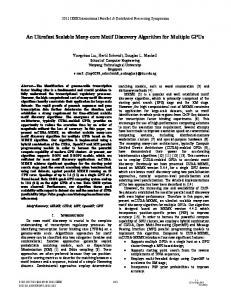
Figure 1: The process of calculating the PFM. (a) The input sequences. (b) The aligned substrings. (c) The count matrix. (d) The position frequency matrix.

In order to overcome these shortcomings, in this paper, we propose an entropy-based position projection algorithm for motif discovery, named EPP. We design a projection method to divide the dataset into candidate subsets by utilizing the relative entropy in each position of motif. Then, EPP filters the candidate subsets and refines the subsets by searching all the possible instances. We consider intramotif dependency in statistics model and calculate the average loglikelihood ratio to combine the short motif. Our algorithm can apply to OOPS, ZOOPS, and TCM sequence model through the threshold setting. Experimental results on real DNA sequences, Tompa data, and ChIP-seq data demonstrate that EPP is advantageous to deal with the motif discovery problem and outperforms current widely used approximate algorithms.

2. Materials and Methods 2.1. Notations. Given an input set of sequences S = {𝑆𝑖 | 𝑖 = 1, 2, 3, . . . , 𝑡} over the alphabet Σ, the length of sequence 𝑆𝑖 is 𝑛𝑖 , the length of the motif to be discovered is 𝑙, and the number of mutations allowed is 𝑑. The substring, 𝑥𝑖𝑗 = (𝑠𝑖𝑗 , 𝑠𝑖,𝑗+1 , . . . , 𝑠𝑖,𝑗+𝑙−1 ), starting at position 𝑗 of the 𝑖th sequence is defined as an 𝑙-mer. For sequence 𝑠𝑖 , there are 𝑛𝑖−𝑙+1 substrings of length 𝑙. Let set X be the set of all the substrings of S. 𝑞 is the projection position. Here, |Σ| = 4 for DNA datasets and |Σ| = 20 for the protein sets. 2.2. Motif Representation. Generally, a motif can be drawn from a multinomial distribution [16], 𝐹 = (𝑓1𝑘 , . . . , 𝑓𝑤𝑘 , . . . , 𝑓𝑙𝑘 ) (𝑘 ∈ Σ), where 𝑓𝑤𝑘 represents the probability of nucleotide 𝑘 preference at the 𝑤th position of the motif and 𝑓0𝑘 represents the background probability of nucleotide 𝑘. The position frequency matrix (PFM) F can be obtained by calculating the frequency of each nucleotide 𝑘 (𝑘 ∈ Σ) at each aligned site: 𝑓𝑤𝑘 =

𝑁𝑤𝑘 + 𝜀 , ∑𝑘∈Σ 𝑁𝑤𝑘 + 4𝜀

(1)

where 𝑁𝑤𝑘 is the count of an observed nucleotide 𝑘 at position 𝑤 and 𝜀 indicates the pseudocounts to deal with the zero frequencies. Figure 1 describes how to calculate the PFM through the input sequences. Information content (IC) is a measure to rank the motif conservation [17]. Motifs with higher IC represent they have more specific binding preferences. Suppose we have a motif

built from the PFM of the selected substrings; the information content of the 𝑤th position of the motif is defined as 𝐼𝑤 = ∑ 𝑓𝑤𝑘 log ( 𝑘∈Σ

𝑓𝑤𝑘 ). 𝑓0𝑘

(2)

Due to the independence of the positions of the motif, the information content of motif is 𝑙

𝐼 = ∑ 𝐼𝑤 .

(3)

𝑤=1

The IC can be used to rank motifs with the same length l. However, some researches indicate that the commonly multinomial distribution model may be too simplistic in identifying the binding motifs, while some positions of TF binding motif exert an interdependent effect on binding affinities of TFs [18, 19]. To provide a better result of motifs identification, a more sophisticated model that involves the intramotif dependency should be considered. Intramotif dependency considers that the frequency of nucleotide combinations spanning several positions deviates from the expected frequency under the independent motif distribution [20]. For example, if the frequency of two nucleotides, “GT,” in a pair of positions is much higher or lower than the product of frequency of “G” in the first position and the frequency of “T” in the second position, we infer that these two positions are dependent. Therefore, the log-likelihood of nucleotides 𝑠𝑖 and 𝑠𝑖+1 is 𝑝 (𝑠𝑖 , 𝑠𝑖+1 ) = log

Φ𝑖,𝑖+1 (𝑠𝑖 , 𝑠𝑖+1 ) , Φ0 (𝑠𝑖 , 𝑠𝑖+1 )

(4)

where Φ𝑖,𝑖+1 represents the probability of the nucleotide pair at 𝑖th and (𝑖 + 1)th position of the motif and Φ0 represents the background probability of the nucleotide pair. Then, the conditional probability of the substring 𝑥 is 𝑝 (𝑥 | 𝐹) = log

∑𝑙𝑤=1 ∑𝑘∈Σ 𝑓𝑤𝑘 ⋅ ∑𝑙−1 𝑤=1 ∑𝑘1 ,𝑘2 ∈Σ Φ𝑤,𝑤+1 (𝑘1 , 𝑘2 ) 𝑝0 (𝑥)

,

(5)

where 𝑝0 (𝑥𝑖𝑗 ) is the joint probability under the corresponding background distribution 𝑓0 . In this paper, we use the third-order Markov model to characterize the background sequence and improve the sensitivity and specificity of identifying motifs. The probability of the substring

BioMed Research International

3

𝑥 (𝑠𝑖𝑗 , 𝑠𝑖,𝑗+1 , . . . , 𝑠𝑖,𝑗+𝑙−1 ) in the background under a thirdorder Markov model is 𝑝0 (𝑥) = 𝑝 (𝑠𝑖 ) 𝑝 (𝑠𝑖+1 | 𝑠𝑖 ) 𝑝 (𝑠𝑖+2 | 𝑠𝑖,𝑠𝑖+1 ) ⋅ ⋅ ⋅ 𝑝 (𝑠𝑖+𝑙−1 | 𝑠𝑖+𝑙−2 , 𝑠𝑖+𝑙−3 , 𝑠𝑖+𝑙−4 ) .

(6)

So the information content can be represented as 𝐼 = avg ∑ 𝑝 (𝑥 | 𝐹) log (

𝑝 (𝑥 | 𝐹) ). 𝑝0 (𝑥)

(7)

Based on the substring statistical significance representation, we present a novel entropy-based position projection algorithm (EPP). EPP aims to solve the motif identification problem and make a good trade-off between accuracy and efficiency, which is detailedly described as follows. EPP Algorithm Step 1 (the cluster projection process). Since the random initial state contains too much noise information, how to choose a good initial state to make refinement quickly converge to a local optimal solution becomes essential. Obviously, the (𝑛𝑖 − 𝑙 + 1)𝑡 ways of selecting the l-mers from all substrings to constitute the initial state are too large. Here, we designed a cluster projection method to initialize the parameters: (1) Draw all the substrings from dataset S to form a new set X, X = {𝑥𝑛 | 𝑛 = ∑(𝑛𝑖 − 𝑙 + 1)}, where 𝑥𝑛 represents an 𝑙-mer. (2) Calculate the relative entropy of each position in the set X: 𝐻𝑤 = ∑ 𝑓𝑤𝑘 log ( 𝑘∈Σ

𝑓𝑤𝑘 ), 𝑓0𝑘

(𝑤 = 1, . . . , 𝑙) .

(8)

(3) Select the position 𝑞 of the maximum relative entropy as the projection position, 𝑞 = argmax𝑤=1,...,𝑙 {𝐻𝑤 }. The collection set X is divided into four subsets through the projection process: the first subset 𝑋1 contains all the 𝑙-mers of appearing base “A” in position 𝑞. Similarly, the subsets 𝑋2 , 𝑋3 , and 𝑋4 contain all the 𝑙-mers of appearing bases “C,” “G,” and “T” in position 𝑞, respectively. (4) We set two thresholds max size and min size to check the size of the subsets {𝑋1 , 𝑋2 , 𝑋3 , 𝑋4 }. For example, if |𝑋1 | < min size, we abandon 𝑋1 . That is, 𝑋1 is too small to contain enough motif instances, which means a transcription factor cannot be combined with sufficient sequences; if |𝑋1 | > max size, the subset has much unnecessary background noise, the algorithm should be back to (2), and we find a new projection position to further divide 𝑋1 ; if min size ≤ |𝑋1 | ≤ max size, we consider 𝑋1 is qualified and store it into a candidate set {𝑐𝑚 }. The setting of max size and min size will be described in next section. Figure 2 shows an example of the cluster projection process. Figure 2(a) describes the set X derived from S; we choose the fifth position for projection. Figure 2(b) shows the four subsets divided from X; the fifth positon of each subset is the observing letters “A,” “C,” “G,” and “T,” respectively.

Then, we calculated relative entropy and chose the second, the third, and the fourth position of each subset to project. After several projection processes (Figure 2(c)), we obtain a candidate set {𝑐𝑚 } as shown in Figure 2(d). In the worst case, the maximum number of candidate subsets is 𝑛/min size 𝑛 is the number of all substrings (𝑙mer). However, in practice, the number of candidate subsets will be much less than this number, such that when the number of substrings is 105 , the number of candidate subsets is ultimately only a few hundred. Step 2 (filter the candidate set). The candidate set {𝑐𝑚 } is constituted by a series of cluster subsets which form by the similar substrings of the same letters at several positons. However, the candidate set still contains the useless subsets made up by the background. It will cost a lot to refine these background subsets and it is necessary to filter them. Because the projection process calculates the relative entropy to choose the position, it can measure the statistical significance but cannot reflect the complexity of substrings. In order to evaluate the complexity of each subset, we employ the common single-string score [21] as another measure. 𝑙 1 𝑙 ) 𝐽 (𝑚) = ( ) ∏ ( 𝑙 4 𝑘∈Σ ∑𝑤=1 𝑓𝑤𝑘

∑𝑙𝑤=1 𝑓𝑤𝑘

.

(9)

So we filter each subset of {𝑐𝑚 } by computing the complexity function (9) and the content information (7) as follows: (1) Calculate the complexity score of each subset in {𝑐𝑚 }, denoted by 𝐽(𝑚): 𝐽 (𝑚) =

1 ∑ 𝐽 (𝑚) , |𝑚|

(10)

where |𝑚| represents the cardinality of {𝑐𝑚 } and 𝜑𝐽 represents the radius of complexity. 󵄨 󵄨 𝜑𝐽 = max (󵄨󵄨󵄨󵄨max (𝐽 (𝑚) − 𝐽 (𝑚))󵄨󵄨󵄨󵄨 , 󵄨󵄨 󵄨 󵄨󵄨min (𝐽 (𝑚) − 𝐽 (𝑚))󵄨󵄨󵄨) . 󵄨 󵄨

(11)

(2) Calculate the content information of each class in {𝑐𝑚 }, denoted by 𝐼(𝑚): 𝐼 (𝑚) =

1 ∑ 𝐼 (𝑚) . |𝑚|

(12)

Similarly, let 𝜑IC be the radius of IC: 󵄨 󵄨 𝜑IC = max (󵄨󵄨󵄨󵄨max (𝐼 (𝑚) − 𝐼 (𝑚))󵄨󵄨󵄨󵄨 , 󵄨󵄨 󵄨 󵄨󵄨min (𝐼 (𝑚) − 𝐼 (𝑚))󵄨󵄨󵄨) . 󵄨 󵄨

(13)

(3) For each candidate subset in {𝑐𝑚 }, if it satisfies 󵄨 󵄨󵄨 󵄨󵄨𝐽 (𝑚) − 𝐽 (𝑚)󵄨󵄨󵄨 > 𝜑𝐽 && 󵄨 󵄨

󵄨 󵄨󵄨 󵄨󵄨𝐼 (𝑚) − 𝐼 (𝑚)󵄨󵄨󵄨 > 𝜑IC , 󵄨 󵄨

(14)

this subset is considered qualified and saved into G = {𝐺V }.

4


(a)

GGCGTGT GCGTGTT CGTGTTT GTGTTTC .. .

𝐒

AGTCTAT GTCTATT TCTATTT .. .

...GGCGTGTTTCCCTTTTAGGAAAAGTGATT... ...CTAATTTACCCAGAAAGGAAATTTCCTT... ...AGTTAGTCTATTTTTTCATTTATATAGTA... .. .

𝐒→ 𝐗

GCATTGG CATTGGT ATTGGTT

...GATAGGGCTTTCTGAGCTCTCCTCCCCCT... ...ATAGTTATTGCCATCCTTTAGCATTGGTT...

TAGGAAA TTTTAGG AGTGATT ACCCAGA .. .

(b)

GTTTCCC ATTTCCT TAGTCTA AGGGCTT .. .

q21 = 2

(c)

q1 = 5

TTTAGGA AAAAGTG AAGTGAT CCCAGAA .. .

q22 = 2

CCATCCT

TAGCATT

𝐗

GGCGTGT AAAGTGA CTAATTT GTTATTG .. .

q23 = 3

q24 = 4

AGCATTG

TATTGCC

...A...A...

...C...A...

...G...A...

...T...A...

...A...C...

...C...C...

...G...C...

...T...C...

...A...G...

...C...G...

...G...G...

...T...G...

...A...T...

...C...T...

...G...T...

...T...T...

.. .

.. .

.. .

.. .

.. .

.. .

.. .

.. .

.. .

.. .

.. .

.. .

.. .

.. .

.. .

.. .

.. .

.. .

.. .

···

.. .

···

(d)

···

{cm }

Figure 2: The process of cluster projection.

Step 3 (refine the qualified subsets). Assume each qualified subset 𝐺V corresponds to a motif; the substrings of the qualified subset should be the motif instances. In fact, we found that the qualified subset contains several fake motif instances generated by the background sequences, while some instances may be missed by the projection and filter processes and are not in the qualified subsets. Therefore, in this step, we remove the fake instances and add the missing ones to refine each qualified subset. As the previous study [22], we know the instances 𝑀1 and 𝑀2 of the same motif should be satisfied 𝐷𝐻(𝑀1 , 𝑀2 ) ≤ 2𝑑, where 𝐷𝐻(⋅) is the function of measuring the hamming distance between two substrings. For each qualified subset in 𝐺V , if the substring of the qualified subset satisfies the hamming distance less than or equal to 2d from the others, we keep it in the subset; otherwise, we remove it from the subset. For each fixed 𝑙, the value of 𝑑 is usually set as 𝑑 < 𝑙 = 2. In this way, the real motif instances must be in one qualified subset. Then, we search all the possible instances from X and add them into 𝐺V . The possible instances should satisfy the following two conditions. First, the instance 𝑥 satisfies 1 𝐷𝐻 (𝑥, 󵄨󵄨 󵄨󵄨 ∑ 𝑔) ≤ 2𝑑, 󵄨󵄨𝐺V 󵄨󵄨 𝑔∈𝐺V

(15)

where |𝐺V | is the cardinality of 𝐺V and 𝑔 represents one instance in 𝐺V . Second, adding the instance 𝑥 increases the information content (7) of 𝐺V . These limiting conditions greatly reduce the search space, and we can obtain the refinements for each qualified subset after removing and adding the substrings. In addition, if the qualified subset is too small (less than min size), it indeed does not make sense to contain the real motif instances. We will not refine the small qualified subset and drop it. Step 4 (predict the longer motif). See each qualified subset as a seed, its PWM can be computed by the steps above, while the corresponding motif with high information content can also be calculated. However, the qualified subsets may represent the similar motifs with a few letters varying as previous studies [23, 24]. In order to eliminate redundant motif information and expand the short motif to form longer motif, we combine the similar motifs having the long common-overlap segments by utilizing a metric of computing the average log-likelihood ratio (ALLR) [25]: ALLR (𝑥1 [𝑤1 ] , 𝑥2 [𝑤2 ]) =

∑𝑘 𝑁𝑤2 𝑘 ln (𝑓𝑤1 𝑘 /𝑓0𝑘 ) + ∑𝑘 𝑁𝑤1 𝑘 ln (𝑓𝑤2 𝑘 /𝑓0𝑘 ) ∑𝑘 𝑁𝑤1 𝑘 + 𝑁𝑤2 𝑘

,

(16)


5

Input: the dataset S, motif length 𝑙. Output: the motifs set 𝐶 (1) X ← all the substrings length 𝑙 from S (2) {𝑐𝑚 } ← 0 // the candidate set (3) {𝐺V } ← 0 // the qualified set (4) 𝑞𝑢𝑒𝑢𝑒 ← X (5) WHILE queue is not empty DO (6) 𝑐 ← DEQUENE(queue) (7) IF |𝑐| < min size (8) abandon c (9) IF min size ≤ |𝑐| ≤ max size (10) {𝑐𝑚 } ← 𝑐 (11) IF |𝑐| > max size (12) select position 𝑞 in 𝑐 𝑎 =A 𝑎 =C 𝑎 =G 𝑎 =T (13) {𝑐(𝑥𝑖 𝑞 ), 𝑐(𝑥𝑖 𝑞 ), 𝑐(𝑥𝑖 𝑞 ), 𝑐(𝑥𝑖 𝑞 )} ← 𝑝𝑎𝑟𝑡𝑖𝑡𝑖𝑜𝑛(𝑐) 𝑎 =A 𝑎 =C 𝑎 =G 𝑎 =T (14) ENQUENE{𝑐(𝑥𝑖 𝑞 ), 𝑐(𝑥𝑖 𝑞 ), 𝑐(𝑥𝑖 𝑞 ), 𝑐(𝑥𝑖 𝑞 )} (15) For each 𝑐𝑚 do (16) IF |𝐽(𝑚) − 𝐽(𝑚)| > 𝜑𝐽 && |𝐼(𝑚) − 𝐼(𝑚)| > 𝜑IC (17) {𝐺V } ← 𝑐𝑚 (18) For each 𝐺V do (19) IF 𝐷𝐻(𝑥, 𝑔) > 2𝑑 (20) remove 𝑥 from 𝐺V (21) IF 𝑥 can increase 𝐼 = avg ∑ 𝑝(𝑥 | 𝐹) log(𝑝(𝑥 | 𝐹)/𝑝0 (𝑥)) (22) add 𝑥 into 𝐺V (23) evaluate the PWM ΘV and 𝐼V . (24) combine the similarly 𝐺V (25) add 𝑥motif formed by ΘV of top 𝐼V to C. (26) return C Algorithm 1

where 𝑓0𝑘 is the background frequency of base 𝑘 and 𝑁𝑤1 𝑘 /𝑁𝑤2 𝑘 and 𝑓𝑤1 𝑘 /𝑓𝑤2 𝑘 are the count and frequency of base 𝑘 at the 𝑤1 th/𝑤2 th position of 𝑥1 /𝑥2 . Since the length of predicted motifs may be different, we use the minimum distance between motifs among all possible overlaps of motifs 𝑥1 and 𝑥2 that the aligned segment is 6. Thus, we calculate the similarity score of 𝑥1 and 𝑥2 by (17), where 𝑙𝑠 denotes the length of the segment: sim (𝑥1 , 𝑥2 ) 𝑙𝑠 −1

= max ( ∑ ALLR (𝑥1 [𝑤1 + ℎ] , 𝑥2 [𝑤2 + ℎ])) . 𝑤1 ,𝑤2

(17)

ℎ

Suppose the number of motifs to find is 𝑢; when a new motif is found, we first check whether there is a similar motif. If the similar motif exists, we combine them and obtain the longer motif; if the similar motif does not exist, we keep the new motif and replace the motif with minimum information content. In this way, we ensure the 𝑢 motifs are different which are also have the information contents as high as possible. In practice, we finally combine and generate at least 20 top information content motifs as the outputs. The whole algorithm of EPP is described in Algorithm 1. In Step 1, lines (1) to (14), we make the projections to obtain candidate sets; then lines (15) to (17) are the step to filter candidate sets to get the qualified subsets; lines (18) to

(23) are the step to refine each qualified subset; at last, lines (24) to (26) are the step to combine the similar motifs and output the results.

3. Results and Discussion The parameters we can get from the input dataset include the number of sequences 𝑡 and the length of each sequence 𝑛𝑖 (𝑖 = 1, . . . , 𝑡); the motif length 𝑙 is known (6–30 bps). Based on these parameters, we draw the set X and then start the projection process. The times of projection and the number of the candidate subsets are depending on the parameters of max size and min size. We hope that the candidate subsets containing the true motif have the motif instances as more as possible and have less influence by the background. Thus, for different sequence models, the parameters of max size and min size are flexibly setting in this way. For the OOPS model (one occurrence of motif instance per sequence), we take max size = t and min size = 3𝑡/4; for the ZOOPS model (zeroor one-motif occurrences per dataset sequence), the number of motif instances is less than the number of sequences and we take max size = 𝑡 and min size = t/2; for TCM (two-component mixture) model, there are zero or more nonoverlapping occurrences. Generally, we take max size = 3t/2 and min size = 𝑡. We first use six real DNA datasets to test the performance of our algorithm, including CREB, CRP, MEF2, MYOD, SRF,

6

BioMed Research International Table 1: The information of six DNA datasets.

Datasets

𝑡

𝑛

𝑙

𝑧

𝑧 avg

CREB CRP MEF2 MYOD SRF TBP

17 18 17 17 20 95

200 105 200 200 200 200

8 18 10 6 10 7

19 23 17 21 36 95

1.12 1.28 1 1.23 1.8 1

and TBP [26–28]. These datasets contain the sequences of different species, in which motif length varies from 6 to 18 and the number of motif instances is from 17 to 95. Note that, in CREM and CPR datasets, some sequences have two motifs, and in MYOD and SRF datasets, the number of motifs is more than two in some sequences. Using these datasets to test, we can check the performance and stability of our algorithm in different species. And the site information tagged in the dataset can help us have a better performance analysis and compare with other algorithms. The information of the six datasets is shown in Table 1. Where 𝑡 represents the sequence number, 𝑛 is the sequence length, 𝑙 is the motif length, 𝑧 is the number of motif instances in the dataset, and 𝑧 avg is the average number of motif instances in each sequence. We compare EPP algorithm with the widely used algorithms, MEME [10], GAME [29], VINE [14], and APMotif [15]. In order to achieve a fair comparison, we use the same motif length for each dataset and use the prior information as less as possible. We choose groups of different initiate sites for multirunning MEME because of the sensitive with initiate conditions. For the genetic-based algorithm GAME, the results are influence by the random seeds; thus, we run the algorithm 20 times and take the average. In each run, the search quantity of motif sets of GAME is 3 × 107 . In order to evaluate the performance of the algorithms, we employ an evaluation method mixing the nucleotide level and the site level [30]. That is, if the predict sites and the real sites are shifting in three bases, it is a true instance. We employ three measures, Precision, Recall, and 𝐹 score [31], which are defined as follows: Precision =

|correct motif| , |motif found|

Recall =

|correct motif| , |ture found|

𝐹 score = 2 ×

(18)

Precision × Recall . Precision + Recall

Here, Precision represents the probability of predicted instances which is influenced by false positive instances. Recall represents the probability of true positive instances. And 𝐹 score is a measure which makes a balance between Precision and Recall, which reduces the influence of false positive. A high 𝐹 score means the algorithm has good performance in both Precision and Recall.

Table 2 shows the results of MEME, GAME, VINE, APMotif, and EPP. It can be seen that EPP has a good performance of Precision on MYOD (0.78) and SRP (0.95). MEME has a high Precision on CREB (0.93), MEF2 (0.93), and TBP (0.83). VINE has a high Precision on CRP (0.94). In the respect of Recall, our algorithm performs well on CREB (0.90), CRP (0.79), MEF2 (0.94), and SFR (0.97). APMotif has the same Recall (0.94) on MEF2 with EPP. And VINE performs well on MYOD (0.86) and TBP (0.87). On the aspect of Precision and Recall, we can see that EPP has relatively small influence by the background. In the predicted instances, the true motif instances occupy a larger proportion. So on the aspect of 𝐹 score, our algorithm has the best performance among the five algorithms; only APMotif has the same value on MEF2. The comparison of Precision, Recall, and 𝐹 score is shown in Figure 3; we can find EPP has a stable performance on the average and performs well than the current widely used motif finding algorithms. Table 3 shows the amount of subsets and the 𝑙-mers in each step, including the total 𝑙-mers, the thresholds of min size and max size, the amount of candidate subsets and qualified subsets, the 𝑙-mers in the qualified subsets, and the reducing number of 𝑙-mers. We can see that the our algorithm eliminates most of the candidate subsets by the projection step and the filter step; only dozens of subsets need to be refined. Meanwhile, the amount of 𝑙-mers has a great reduction, which is more than 90%. Such as TBP dataset, the amount of 𝑙-mers reduces by 99% and only two subsets need the refinement. The running times of the datasets testing above are shown in Table 4. We implement EPP and APMotif in MATLAB under Windows. GAME is implemented in C under Linux. MEME and VINE are implemented through the website version. It is unfair to compare these algorithms implemented in different software, especially compared with website version. But the running time can explain that our algorithm can find the motifs in a reasonable and acceptable time. We report the computational time in the same experiment environment (2.67 G Hz CPU and 4 G memory). From Table 4, we can see that GAME and APMotif are obviously slower than EPP. The web version MEME and VINE are faster than EPP for most datasets. However, MEME needs to run several times for the different start points and VINE is a heuristic algorithm which will be slow with the data size increasing. EPP has the best time efficiency for TBP data because of the reduction of 99% redundant information. Besides the six real DNA datasets, we also use the Tompa data to test our algorithm. Tompa data is a standard data for evaluating new design motif finding method, including three types of data: Real, Generic, and Markov. Here, we select Real data which contains 52 groups of real promoter sequences extracted from TRANSFAC database and involves four species: Drosophila melanogaster (dm), Mouse (mus), Human (hm), and Saccharomyces cerevisiae (yst). It should be noted that some datasets of Tompa only have one sequence, such as dm02r and dm06r. Not each sequence contains the motif, such as dm01r, hm06r, hm11r, mus07r, and yst01r. And for most of the Tompa datasets, each sequence contains more than one motif, like hm08r, hm10r, mus11r, yst03r, and yst05r.


7

Table 2: The comparison of MEME, GAME, VINE, APMotif, and EPP on six DNA datasets. Datasets

P 0.93 0.89 0.93 0.60 0.74 0.83 0.82

CREB CRP MEF2 MYOD SRF TBP Average

MEME R 0.68 0.67 0.82 0.28 0.89 0.69 0.56

GAME R 0.79 0.78 0.80 0.48 0.92 0.77 0.77

P 0.68 0.79 0.82 0.48 0.70 0.78 0.72

F 0.73 0.78 0.81 0.48 0.80 0.77 0.74

VINE R 0.80 0.70 0.88 0.86 0.94 0.87 0.84

P 0.72 0.94 0.88 0.47 0.92 0.74 0.78

Precision comparison

1 0.9

0.9

0.8

0.8

0.7

0.7

0.6

0.5

0.4

0.4

CREB CRP MEF2 MYOD SRF Datasets MEME GAME VINE

P 0.70 0.86 0.84 0.60 0.88 0.72 0.77

APMotif R 0.84 0.72 0.94 0.52 0.90 0.80 0.79

0.3

TBP Average

F 0.76 0.78 0.89 0.56 0.89 0.76 0.78

P 0.74 0.83 0.84 0.78 0.95 0.82 0.83

EPP R 0.90 0.79 0.94 0.68 0.97 0.81 0.85

F 0.81 0.81 0.89 0.82 0.96 0.82 0.85

Recall comparison

0.6

0.5

0.3

F 0.76 0.80 0.88 0.61 0.93 0.80 0.81

1

Recall

Precision

F 0.78 0.76 0.88 0.38 0.81 0.76 0.73


APMotif EPP (a)

TBP Average

APMotif EPP (b)

F score comparison

1 0.9

F score

0.8 0.7 0.6 0.5 0.4 0.3


TBP Average

APMotif EPP (c)

Figure 3: The accuracy comparison of MEME, GAME, VINE, APMotif, and EPP. (a) Precision comparison. (b) Recall comparison. (c) 𝐹 score comparison.

8

BioMed Research International Table 3: The subsets and 𝑙-mers amount of EPP.

Datasets

Total 𝑙-mers

[min size, max size]

The number of candidate subsets

The number of qualified subsets

The 𝑙-mers in qualified subsets

Reducing amount of 𝑙-mers

CREB CRP MEF2 MYOD SRF TBP

3294 1584 3247 3315 3820 18430

[15, 19] [16, 24] [9, 17] [17, 23] [20, 30] [80, 95]

66 31 176 55 73 32

4 5 33 6 13 2

65 104 335 111 310 175

98% 98% 90% 97% 92% 99%

Table 4: The computational time comparison. Datasets CREB CRP MEF2 MYOD SRF TBP

MEME 1.52 0.60 2.01 2.25 2.12 39.05

GAME 134.00 391.04 113.25 96.08 223.56 786.32

VINE 4.82 2.61 7.37 8.25 10.11 55.53

APMotif 71.23 97.04 135.83 68.36 147.29 280.43

EPP 17.52 8.91 21.91 30.27 28.28 10.83

Motifs are difficult to identify for the weak conservation in Tompa data. Thus, we select a part of the datasets to test, which are dm01r, dm02r, dm03r, dm04r, dm05r, and dm06r in Dm species; mus01r, mus03r, mus05r, mus06r, mus11r, and mus12r in Mus species; hm01r, hm07r, hm08r, hm10r, hm17r, hm22r, hm23r, and hm24r in Hm species; yst01r, yst02r, yst03r, yst04r, yst05r, yst06r, yst08r, and yst09r in Yst species (Figure 4). We use the measure based on the nucleotide level to evaluate the performance, because the number of motifs and the length of motifs are different in each sequence. 𝑁PC =

𝑛TP , (𝑛TP + 𝑛FP + 𝑛FN)

(19)

where 𝑛TP (true positive) represents the real sites in the predicted sites; 𝑛FP (false positive) are the fake sites in the predicted sites; 𝑛FN (false negative) represents the fake sites that do not predict. We also choose MEME as the reference algorithm to compare the performances. The length of motif ranges from 6 to 30 bps, and we output the best result. Figure 3 is the results of EPP and MEME. We can see that both EPP and MEME are hard to find the motifs in the one sequence data sets, such as dm02r and dm06r. For the datasets dm03r, dm04r, and dm05r, some sequences have several motifs but some sequences have no motif; for example, the third sequence of dm05r contains 9 motifs. This motif distribution makes it difficult to identify. Thus, both EPP and MEME have poor effect for the Dm spices. For the Hm spices, one notable feature is that the length of motifs changes a lot; for example, the motifs of hm01r range from 7 to 56 bps. We use the fixed motif length as before which can only predict a part of segment overlapping with the true motif. However, for the data motif length changing relatively small, like hm17r (10–17 bps), both EPP and MEME have the best results. And EPP has a higher accuracy than MEME in the Hm spices. For the Mus and the Yst data, most of the datasets contain less than 10 sequences (expect mus11r, yst03r, yst08r, and yst09r),

Table 5: The performance coefficient of MEME, VINE, and EPP on the synthetic datasets. Datasets Width Short Middle Long Short Middle Long

Con Low Low Low High High High

MEME 0.32 0.88 0.98 0.91 0.98 1

Algorithm VINE 0.24 0.72 0.88 0.96 0.99 1

EPP 0.32 0.90 0.98 0.98 0.99 1

and most of the sequences have multiple motifs of different lengths. From the experiment results, we find that EPP and MEME have their own advantages for these two species. Through the experiments above, we can see the existing algorithms have poor performance on Topma data [32]. However, the different algorithms can complement and reinforce each other. For example, for the data mus06r, yst05r, and hm10r, EPP can have an effective prediction but the accuracy of MEME is worse. In recent research, the algorithm like Ensemble which merges the results of different algorithms can improve the accuracy effectively [33]. Moreover, the same results of the different algorithms can also enhance the prediction. In order to show the effect of our algorithm, we also test the synthetic datasets which contain the low and high conservation positions. The synthetic datasets are generated under the following six combinations of three perspectives: (1) motif width: short (8–10 bp), middle (14–16 bp), and long (19– 21 bp); (2) sequence length: 600 and number of sequences: 20; (3) motif conservation: low and high. For each combination, we sample 10 datasets which are generated randomly and embedded with the instances of a random motif. Specifically, in the high conservation aspect, the dominant nucleotide is generated with 0.91 probability on each position of the motif instance (while all other three nucleotides are generated with 0.03 each). In the low conservation aspect, only 60 percent of the positions in the motif instances are as highly conserved as those in the previous high conservation aspect, while the rest 40 percent of the positions are lowly conserved, where the dominant nucleotide is generated only with probability 0.55 (while all other three nucleotides are generated with 0.15 each) in every instance. Table 5 shows the performance coefficient (NPC) of MEME, VINE, and EPP. From the results, we can see that


9 Table 6: Results of the mouse embryonic stem cell data.

Datasets CTCF cMyc Esrrb Klf4 Nanog nMyc Smad1 Oct4 STAT3 Sox2 Tcfcp2l1 Zfx

Length 11 9 11 10 7 10 16 15 9 10 11 10

Seq. # 39601 3422 21644 10872 10342 7181 1126 3775 2546 4525 26907 10336 Dm

0.3 0.25

0.5

0.2

0.4

0.15

0.3

0.1

0.2

0.05

0.1

0 dm01r

dm02r

dm03r

dm04r

dm05r

0 hm01r hm07r hm08r hm10r hm17r hm22r hm23r hm24r Hm data

dm06r

Dm data

EPP MEME

0.3

0.6

0.25

0.5

0.2

0.4 NPC

NPC

EPP MEME

0.15 0.1 0.05 0 mus01r

Weeder TNGCCACCAGGGGGCGCNN CGCACGTGGC GGTCAAGGTCA GGGTGTGGCC CCATTGTCTNNN CGCACGTGGC CCTTTGTTATGCAAAT CTTTGTTATGCAAAT TTTCCNGGAA CATTGTNATGCAAAT CCGGTTCAAACCGG CGCNAGGCCGCG

0.6

NPC

NPC

EPP CCAGAAGAGGGCG GCTCGTGGC GGTCAAGGTCA GGGTGTGGCC CCATTCT CGCACGTGGC CTTTTGTTATTCAAAT CATTGTTATGCAAA TTCCTGGAA TTGTTATGCA CCAGCCTAGCC CTAGGCCGCG

0.3 0.2 0.1

mus03r

mus05r mus06r Mus data

mus011r

mus12r

EPP MEME

0 yst01r

yst02r

yst03r

yst04r yst05r Yst data

yst06r

yst08r

yst09r

EPP MEME

Figure 4: Results of EPP and MEME on Tompa datasets.

all these compared algorithms have good performance on the high conservation dataset. Among these compared algorithms, EPP has the best results on three high conservation datasets (0.98, 0.99, and 1), which are higher than the other three algorithms. For the low conservation datasets, EPP has the highest accuracies among these compared algorithms. However, when the width of motif is short, motif instances are hard to distinguish from the background sequences; the accuracies of all the compared algorithms are low. Meanwhile, we also use 12 TFs in mouse embryonic stem cell ChIP-seq datasets to test our algorithm. ChIP-seq is a technique coupling chromatin immunoprecipitation

experiment with high-throughput sequencing [34, 35], which provides dataset of one or two magnitudes larger than a typical motif discovery dataset and sequences with a high resolution. Therefore, the tradition motif finding algorithms are hard to solve ChIP-seq data for the huge calculation. In order to improve the efficiency of EPP, the original dataset is equally divided into halves: a training set and a testing set. We run the projection and filter steps on the training set to generate the qualified subsets, and then run the refine step to search the instances and construct longer motifs on the testing set. Table 6 shows the results of 12 TFs in mES ChIP-seq datasets discovered by our algorithm with the

10 motifs found by Chen et al. with Weeder [36]. It can be seen that EPP is able to find the motif similar to the published one. Chen et al. report a single motif with Weeder. Besides these primary motifs, our algorithm can find multiple motifs for each TF using the same datasets. For instance, Oct4 and Sox2 often form a heterodimer that binds a Oct4 motif located adjacent to a Sox2 motif, called the Sox-Oct motif [37]. In Sox2 and Oct4 dataset, EPP predicts not only the Sox-Oct composite motif bound by Sox2 and Oct4 complex but also the monomer motifs Sox2 (CCATTGTT) and Oct4 (TATGCAAAT). As discussed by Chen et al., Smad1 and Nanog frequently bind the same regions as Oct4 and Sox2, which raises a particular difficulty for motif discovery [38]. In Smad1 dataset, our algorithm finds motif “CCTTTGTC,” which matches a Sox2 motif and demonstrates the frequent cobinding relationship of Smad1 and Sox2 TFs. Furthermore, our algorithm was able to find the Nanog motif “CCATCAA,” which corresponds to an experimentally validated alternative Nanog motif [39]. In summary, EPP is a competitive algorithm to deal with motif discovery problem; our method has the following advantages: (1) the projection which deals with all the substrings does not miss any information in the data. That is, this step guarantees each substring may exist in a candidate subset. (2) The goal of finding motif is to find the substrings having the maximum IC, and the process of selecting the projection positon is also a part of maximizing IC. (3) The size of candidate subsets depends on the thresholds [min size, max size]. If a candidate subset is too large, it will contain too much background information. We continue to divide it; if a candidate subset is too small, the substring in it may be not enough to represent an effective motif. We abandon it. In some cases, motif instance may exist in the abandoned subset, but it still can make up by other subsets containing the motif instance. In the worst case, the number of the candidate subsets is n/min size, where n is the number of all substrings. However, in practice, this number will drastically reduce. The number of candidate subsets may be only a few hundred for 106 substrings. (4) There are often some meaningless DNA segments in real data, such as duplicate “AAAAAAAAAA” or “CGCGCGCGCG.” These segments will generate the same duplicate substrings which cause redundant computation. Through the projection step of our algorithm, these segments will be very easy to find and discard. In addition, the computation complexity of EPP mainly depends on projection step and refinement step. Suppose the time of projection is ℎ, in each projection, the computation complexity of calculating relative entropy is O(nl); then, the computation complexity of the projection step is O(hnl). Since the order of magnitude of ℎ and 𝑙 is 10, and 𝑛 is usually less than 106 , the order of magnitude of projection is about 108 . In the refinement, the number of qualified subsets is about 102 for 106 substrings. the computation complexity of refinement in each qualified subset is O(nl). So the order of magnitude of refinement is 108 which is totally acceptable.


4. Conclusions We propose a new probability algorithm named EPP for identifying motifs in DNA datasets. EPP presents a new entropy-based position projection to divide original dataset and remove a large amount of redundant information. Experimental results show that EPP is able to efficiently and effectively identify motifs in DNA sequences and ChIP-seq datasets. However, the functions of some motifs are still unknown; the analysis of motifs in these complex transcriptional regions is needed. In addition, with the increase of data size, designing the parallel algorithm to handle big data is also a key issue for the future study.

Competing Interests The authors declare that there is no conflict of interests regarding the publication of this article.

Acknowledgments This work was supported by the Fundamental Research Funds for the Central Universities (nos. 310832161008, 310832163403), the Natural Science Foundation of Shaanxi (nos. 2016JQ6075, 2016JM6059), and the National Natural Science Foundation of China (no. 51505037).

References [1] P. A. Pevzner and S. H. Sze, “Combinatorial approaches to finding subtle signals in DNA sequences,” in Proceedings of the 8th International Conference on Intelligient Systems for Molecular Biology, pp. 269–278, AAAI Press, 2000. [2] F. Zambelli, G. Pesole, and G. Pavesi, “Motif discovery and transcription factor binding sites before and after the nextgeneration sequencing era,” Briefings in Bioinformatics, vol. 14, no. 2, pp. 225–237, 2013. [3] T. D. Schneider, “Consensus sequence zen,” Applied Bioinformaitics, vol. 1, no. 3, pp. 111–119, 2002. [4] S. Tanaka, “Improved exact enumerative algorithms for the planted (l, d)-motif search problem,” IEEE/ACM Transactions on Computational Biology and Bioinformatics, vol. 11, no. 2, pp. 361–374, 2014. [5] Y. Zhang and P. Wang, “A fast cluster motif finding algorithm for ChIP-Seq data sets,” BioMed Research International, vol. 2015, Article ID 218068, 10 pages, 2015. [6] Q. Yu, H. Huo, X. Chen, H. Guo, J. S. Vitter, and J. Huan, “An efficient algorithm for discovering motifs in large DNA data sets,” IEEE Transactions on NanoBioscience, vol. 14, no. 5, pp. 535–544, 2015. [7] C. Jia, M. B. Carson, Y. Wang, Y. Lin, and H. Lu, “A new exhaustive method and strategy for finding motifs in ChIP-enriched regions,” PLoS ONE, vol. 9, no. 1, Article ID e86044, 2014. [8] S. P. Pissis, “MoTeX-II: structured MoTif eXtraction from largescale datasets,” BMC Bioinformatics, vol. 15, no. 1, article 235, 2014. [9] T. L. Bailey, P. Krajewski, I. Ladunga et al., “Practical guidelines for the comprehensive analysis of ChIP-seq data,” PLoS Computational Biology, vol. 9, no. 11, Article ID e1003326, 2013.

BioMed Research International [10] T. L. Bailey and C. Elkan, “Fitting a mixture model by expectation maximization to discover motifs in biopolymers,” in Proceedings of the 2nd International Conference on Intelligent Systems for Molecular Biology, pp. 28–36, California, Calif, USA, 1994. [11] C. E. Lawrence, S. F. Altschul, M. S. Boguski, J. S. Liu, A. F. Neuwald, and J. C. Wootton, “Detecting subtle sequence signals: a gibbs sampling strategy for multiple alignment,” Science, vol. 262, no. 5131, pp. 208–214, 1993. [12] T. L. Bailey, N. Williams, C. Misleh, and W. W. Li, “MEME: discovering and analyzing DNA and protein sequence motifs,” Nucleic Acids Research, vol. 34, supplement 2, pp. W369–W373, 2006. [13] J. Buhler and M. Tompa, “Finding motifs using random projections,” Journal of Computational Biology, vol. 9, no. 2, pp. 225– 242, 2002. [14] C.-W. Huang, W.-S. Lee, and S.-Y. Hsieh, “An improved heuristic algorithm for finding motif signals in DNA sequences,” IEEE/ACM Transactions on Computational Biology and Bioinformatics, vol. 8, no. 4, pp. 959–975, 2011. [15] C. Sun, H. Huo, Q. Yu, H. Guo, and Z. Sun, “An affinity propagation-based DNA motif discovery algorithm,” BioMed Research International, vol. 2015, Article ID 853461, 10 pages, 2015. [16] J. S. Liu, A. F. Neuwald, and C. E. Lawrence, “Bayesian models for multiple local sequence alignment and gibbs sampling strategies,” Journal of the American Statistical Association, vol. 90, no. 432, pp. 1156–1170, 1995. [17] G. Z. Hertz and G. D. Stormo, “Identifying DNA and protein patterns with statistically significant alignments of multiple sequences,” Bioinformatics, vol. 15, no. 7-8, pp. 563–577, 1999. [18] M. L. Bulyk, P. L. F. Johnson, and G. M. Church, “Nucleotides of transcription factor binding sites exert interdependent effects on the binding affinities of transcription factors,” Nucleic Acids Research, vol. 30, no. 5, pp. 1255–1261, 2002. [19] P. V. Benos, M. L. Bulyk, and G. D. Stormo, “Additivity in protein-DNA interactions: how good an approximation is it?” Nucleic Acids Research, vol. 30, no. 20, pp. 4442–4451, 2002. [20] M. Hu, J. Yu, J. M. G. Taylor, A. M. Chinnaiyan, and Z. S. Qin, “On the detection and refinement of transcription factor binding sites using ChIP-Seq data,” Nucleic Acids Research, vol. 38, no. 7, pp. 2154–2167, 2010. [21] S. Mahony, P. V. Benos, T. J. Smith, and A. Golden, “Selforganizing neural networks to support the discovery of DNAbinding motifs,” Neural Networks, vol. 19, no. 6-7, pp. 950–962, 2006. [22] Y. Zhang, H. Huo, and Q. Yu, “A heuristic cluster-based em algorithm for the planted (l, d) problem,” Journal of Bioinformatics and Computational Biology, vol. 11, no. 4, Article ID 1350009, 19 pages, 2013. [23] T. L. Bailey, M. Bodén, T. Whitington, and P. Machanick, “The value of position-specific priors in motif discovery using MEME,” BMC Bioinformatics, vol. 11, article 179, 2010. [24] S. Georgiev, A. P. Boyle, K. Jayasurya, X. Ding, S. Mukherjee, and U. Ohler, “Evidence-ranked motif identification,” Genome Biology, vol. 11, no. 2, 2010. [25] T. Wang and G. D. Stormo, “Combining phylogenetic data with co-regulated genes to identify regulatory motifs,” Bioinformatics, vol. 19, no. 18, pp. 2369–2380, 2003. [26] C. E. Lawrence and A. A. Reilly, “An expectation maximization (EM) algorithm for the identification and characterization of

11

[27]

[28]

[29]

[30]

[31]

[32]

[33]

[34] [35]

[36]

[37]

[38]

[39]

common sites in unaligned biopolymer sequences,” Proteins: Structure, Function, and Bioinformatics, vol. 7, no. 1, pp. 41–51, 1990. J. S. Liu, “The collapsed Gibbs sampler in Bayesian computations with applications to a gene regulation problem,” Journal of the American Statistical Association, vol. 89, no. 427, pp. 958– 966, 1994. E. Blanco, D. Farré, M. M. Albà, X. Messeguer, and R. Guigó, “ABS: a database of Annotated regulatory Binding Sites from orthologous promoters,” Nucleic Acids Research, vol. 34, supplement 1, pp. D63–D67, 2006. Z. Wei and S. T. Jensen, “GAME: detecting cis-regulatory elements using a genetic algorithm,” Bioinformatics, vol. 22, no. 13, pp. 1577–1584, 2006. T.-M. Chan, K.-S. Leung, and K.-H. Lee, “TFBS identification based on genetic algorithm with combined representations and adaptive post-processing,” Bioinformatics, vol. 24, no. 3, pp. 341– 349, 2008. W. M. Shaw Jr., R. Burgin, and P. Howell, “Performance standards and evaluations in IR test collections: cluster-based retrieval models,” Information Processing and Management, vol. 33, no. 1, pp. 1–14, 1997. M. Tompa, N. Li, T. L. Bailey et al., “Assessing computational tools for the discovery of transcription factor binding sites,” Nature Biotechnology, vol. 23, no. 1, pp. 137–144, 2005. J. Hu, B. Li, and D. Kihara, “Limitations and potentials of current motif discovery algorithms,” Nucleic Acids Research, vol. 33, no. 15, pp. 4899–4913, 2005. E. R. Mardis, “ChIP-seq: welcome to the new frontier,” Nature Methods, vol. 4, no. 8, pp. 613–614, 2007. P. J. Park, “ChIP-seq: advantages and challenges of a maturing technology,” Nature Reviews Genetics, vol. 10, no. 10, pp. 669– 680, 2009. X. Chen, H. Xu, P. Yuan et al., “Integration of External Signaling Pathways with the Core Transcriptional Network in Embryonic Stem Cells,” Cell, vol. 133, no. 6, pp. 1106–1117, 2008. A. Reményi, K. Lins, L. J. Nissen, R. Reinbold, H. R. Schöler, and M. Wilmanns, “Crystal structure of a POU/HMG/DNA ternary complex suggests differential assembly of Oct4 and Sox2 on two enhancers,” Genes and Development, vol. 17, no. 16, pp. 2048– 2059, 2003. M. Thomas-Chollier, C. Herrmann, M. Defrance, O. Sand, D. Thieffry, and J. Van Helden, “RSAT peak-motifs: Motif analysis in full-size ChIP-seq datasets,” Nucleic Acids Research, vol. 40, no. 4, article e31, 2012. X. He, C.-C. Chen, F. Hong et al., “A biophysical model for analysis of transcription factor interaction and binding site arrangement from genome-wide binding data,” PLoS ONE, vol. 4, no. 12, Article ID e8155, 2009.

International Journal of

Peptides

BioMed Research International Hindawi Publishing Corporation http://www.hindawi.com

Volume 2014

Advances in

Stem Cells International Hindawi Publishing Corporation http://www.hindawi.com

Volume 2014

Hindawi Publishing Corporation http://www.hindawi.com

Volume 2014

Virolog y Hindawi Publishing Corporation http://www.hindawi.com


Genomics

Volume 2014


Volume 2014

Journal of

Nucleic Acids

Zoology




Volume 2014

Volume 2014

Submit your manuscripts at http://www.hindawi.com The Scientific World Journal

Journal of

Signal Transduction Hindawi Publishing Corporation http://www.hindawi.com

Genetics Research International Hindawi Publishing Corporation http://www.hindawi.com

Volume 2014

Anatomy Research International Hindawi Publishing Corporation http://www.hindawi.com

Volume 2014

Enzyme Research

Archaea Hindawi Publishing Corporation http://www.hindawi.com


Volume 2014

Volume 2014


Biochemistry Research International


Microbiology Hindawi Publishing Corporation http://www.hindawi.com

Volume 2014


Evolutionary Biology Volume 2014


Volume 2014


Volume 2014

Molecular Biology International Hindawi Publishing Corporation http://www.hindawi.com

Volume 2014

Advances in

Bioinformatics Hindawi Publishing Corporation http://www.hindawi.com

Volume 2014

Journal of

Marine Biology Volume 2014


Volume 2014