conjunction with a simple graphical method of inter- pretation, has proven ... the builder to avoid those problems associated with the ... the excavation of the site.
Downloaded 03/08/15 to 129.123.73.40. Redistribution subject to SEG license or copyright; see Terms of Use at http://library.seg.org/
GEOPHYSICS, VOL. 55. (MAY 1990); P. 514--520,10 FIGS.
An evaluation of Bristow's method for the detection of subsurface cavities
Tony Lowry* and Peter N. Shive*
incorporate geologic noise, the maximum depth at which a cavity can be detected is found to be far less than has been reported in field investigations. In this instance the presence of a cylindrical cavity cannot be discerned beyond a depth to the top approximately equal to the diameter of the cavity, and spherical cavities are indistinguishable at depths much greater than the radius. One should note that the noise field generated for this model may not be representative of what would normally be found in the real earth. In the field, the maximum achievable depth of detection will vary depending on the actual geologic conditions and whether some technique is employed to reduce the effects of noise. In any case, a comparison of traverses using various electrode arrays confirms that the Bristow method is the most satisfactory of the applicable electrical resistivity techniques.
ABSTRACT
The Bristow method, an electrical resistivity technique employing a pole-dipole measurement array in conjunction with a simple graphical method of interpretation, has proven an effective means of locating subsurface cavities. There have been questions, however, regarding the limits of the method and whether the Bristow method is indeed the most suitable of the various electrical resistivity techniques for cavity detection. In hopes of resolving some of the controversy surrounding Bristow's method, resistivity traverses are numerically modeled over spherical and cylindrical cavities given a variety of circumstances. Using a slight variation of Bristow's original interpretive technique on modeled data, the size and location of subsurface cavities can be determined with surprising accuracy. However, when the simulation is altered to
imate position of several known passages. More impressively, he discovered two cavities and verified their existence through drilling and excavation. A few years after its introduction, Bates (1973) used Bristow's method to delineate a number of known cavities. After making some slight modifications, he was also able to locate a relatively small target cavity as well as several anomalous regions which did not correspond with any known cavities. Regrettably, no attempt was made to confirm whether the latter were indeed caves. Several field examinations of the Bristow method, exhibiting varying degrees of success, have since been conducted. In the course of their respective explorations of sites of known subsidence, Fountain et al. (1975) were able to detect both air-filled and mud-filled cavities and Smith (1986) located a solution-filled cavity, all of which were confirmed by drilling. Cooper and Bieganousky (1978) and Ballard (1982) achieved results which are perhaps best regarded as inconclusive. Butler and Murphy (1980) were decidedly unsuc-
INTRODUCTION
The presence of solution features or abandoned mine tunnels beneath a highway, dam, or building can pose a serious threat to the stability of the structure. Investigators have experimented with all manner of geophysical techniques in the search for an inexpensive, reliable means of locating cavities before construction begins, thus permitting the builder to avoid those problems associated with the subsidence or collapse of a structural foundation. Of the various methods which have been applied successfully to detect subsurface cavities, a technique designed by C. M. Bristow (1966) has attracted a great deal of attention. This technique, commonly referred to as the Bristow method, consists of an electrical resistivity approach using a pole-dipole array similar to that popularized by Logn (1954) in conjunction with a simple graphical technique used to interpret the resulting data. Using this method in field studies over karst terrains, Bristow was able to describe the approx-
Manuscript received by the Editor November 28, 1988; revised manuscript received November 7, 1989. *Department of Geology and Geophysics, University of Wyoming, P.O. Box 3006, Laramie, WY 82071. © 1990 Society of Exploration Geophysicists. All rights reserved.
514
Downloaded 03/08/15 to 129.123.73.40. Redistribution subject to SEG license or copyright; see Terms of Use at http://library.seg.org/
Cavity Detection by Bristow's Method
cessful in their attempts to locate several artificially emplaced target cavities, but that particular failure might be ascribed to aggravation of the geologic noise as a result of the excavation of the site. Kirk and Werner (1981), based on their own experiences and published accounts of other investigations, claim a success rate for the method of just over 50 percent. The method of intersecting arcs used to interpret the data, however, has drawn criticism from some researchers (Myers, 1975; Creedy, 1975), who argue that it is based on faulty assumptions and that many of the positive results reported using Bristow's method may well be serendipitous. Discussions probing the capabilities of the Bristow method have focused largely on field investigations in which measurement errors and the complexity of geologic conditions can obscure desired information or even lead to false conclusions. One exception is Spiegel et al. (1980), who detail a numerical technique for modeling arbitrary 3-D anomalous bodies underlying an irregular surface terrain. Owen (1983) also refers to model results in his survey of current methods for detection of tunnels and caves. In this paper, numerical methods are used to model electrical resistivity surveys over spherical and cylindrical subsurface cavities. Bristow's interpretive method is applied to the resulting data, permitting a test of the approach with conditions such as the size and placement of the cavity and the nature of the surrounding material carefully controlled. The resolution of the pole-dipole array is compared to that of other electrode arrays. The maximum depth at which one can reasonably expect to detect a cavity is considered, and the consequences of varying the potential-electrode spacing are explored as well. Based on the results of these models, we suggest how to use Bristow's method most effectively to delineate localized inhomogeneities. THE BRISTOW METHOD
The resistivity technique is one of several electrical prospecting methods for mapping the geoelectric structure of the earth's subsurface. An electric current is injected into the ground via two electrodes (the current electrodes), inducing an electrical potential field in the surrounding earth. The earth's response is measured as a potential drop or voltage across another pair of electrodes, referred to as the potential electrodes. This measurement is then expressed as an apparent resistivity-in essence, the resistivity indicated by the measured voltage given the relative positions of the electrodes and assuming the ground has invariant electrical properties throughout. The apparent resistivity at the point midway between the potential electrodes, denoted Pa' is given by 2'TTV ( 1 ) Pa = / - 1- _ 1- _ 1- + 1rl
r2
r3
'
(1)
r4
in which V is the voltage, / is the current, and the distances r are as shown in Figure 1. Of course, the resistivity is not normally homogeneous in a geologic setting; so if one or more of the electrodes is moved, a different apparent resistivity should be indicated, reflecting in some manner the variation in electrical conductivity of the earth. A number of electrode arrangements are commonly used
515
for resistivity surveying, each with its own strengths and weaknesses. The Bristow method employs a pole-dipole electrode array, in which a monopolar current source is approximated by moving the current sink electrode an effectively infinite distance from its counterpart-in practice, anywhere from five to ten times the distance to be surveyed. Voltage readings are taken at progressively greater distances from the stationary current source along a linear traverse. Because the effects of the current sink electrode are minimized, the apparent resistivity calculation for this array becomes Pa
=
2'TT /
V(~).
(2)
r2 - rl
Generally, a resistivity array is intended to function in one of two capacities. Profiling techniques describe lateral variations in resistivity by maintaining a constant electrode spacing while incrementally advancing the electrode array across the area of interest. Sounding is accomplished by centering the array at a single location and gradually increasing the distance between electrodes in order to reflect changes in resistivity with greater depth. The pole-dipole array as employed by Bristow (1966) does not fit neatly into either category; rather, the technique was designed to trace variations in resistivity with increasing radial distance from the source electrode. Bristow (1966) drew upon this conceptualization in developing his method of intersecting arcs for interpretation of the resistivity data. Reasoning that, in an otherwise homogeneous medium, the source of an apparent resistivity high or low should lie along a circular arc incorporating the anomaly and centered about the current source, the intuitive claim was made that for two or more traverses across a given region the source of the respective anomalies should occur at the intersection of the circular arcs extending from them. The resulting interpretive construction is illustrated in Figure 2. Note, however, that the visualization of the apparent resistivity curve as a reflection of how the earth's resistivity behaves with increasing radial distance from the current source is only an approximation. THE MODELING PROCEDURE
The results cited below were modeled using a 3-D integrated finite-difference numerical scheme similar to that introduced by Dey and Morrison (1979) but made slightly more accurate by incorporating singularity removal. Briefly, a desired distribution of geoelectrical properties is approximated as a finite half-space made up of parallelepiped blocks, with each block being assigned its own discrete resistivity value. The partial differential equation which governs the resistivity problem is given by
v . [u(x)V(x)] =
- /8(x - x,),
in which cr is the conductivity (the inverse of the resistivity and a function of spatial position), is electrical potential (likewise a function of position), lis the injected current, 8 is the delta function, and X s is the spatial position of the current source. This equation is discretized and a surface integral is taken about each nodal point, after which a first-order forward finite-difference approximation is substituted for each partial derivative term. The resulting series of linear
Downloaded 03/08/15 to 129.123.73.40. Redistribution subject to SEG license or copyright; see Terms of Use at http://library.seg.org/
516
Lowry and Shive
equations is solved algebraically for the potential at each of the nodal points. Those wishing a more complete explanation of the mathematical procedure, including a discussion of singularity removal, are referred to Lowry et al. (1989). In the course of developing the numerical scheme, the various sources of error were analyzed extensively in order to maximize the accuracy of the technique. Only a very small fraction of the error was due to computational or machine inaccuracy, a somewhat larger portion was numerical error resulting from the discretization of the problem, and perhaps most of the error derived from other sources such as the approximation of boundary conditions on the partial differential equation. The problem posed herein, i.e., the simulation of a spherical or cylindrical cavity in a medium, involves two additional sources of error. First, a sphere or cylinder cannot be modeled exactly using cubic blocks. For our purposes, a grid mesh of one-tenth the diameter of the object was used. Convergence plots employing decreasing mesh sizes suggest that the improvement which results from using a smaller mesh is relatively slight. However, the computational time
necessary to complete a solution increases rapidly as the number of nodes is increased. The second source of error arises because those blocks having centers which fall within the radius of the sphere or cylinder are assigned "very large" but not infinite resistivity values. The latter is the larger contributor to the total error, but it cannot be avoided within the strictures of the finite-difference modeling scheme used. Even so, the error in the model is acceptably small. When compared to analytically derived solutions, average errors along a resistivity traverse are typically less than 1 percent. A more rigorous examination of the error analysis performed on the numerical method is detailed in Lowry et al. (1989). RESULTS
In hopes of achieving a qualitative feel for some of the capabilities and limitations of the Bristow method, poledipole traverses are modeled over simulated cavities given a variety of circumstances. In each case, a cavity of 1.0 m radius is emplaced within a half-space having a resistivity (or, for those simulations incorporating randomly induced statistical noise, a mean resistivity) of 100 ohm-m, a resistivity magnitude appropriate for limestone. The most obvious means of assessing the Bristow method is to apply the technique to modeled data and compare the position of the interpreted cavity as indicated by the method of intersecting arcs to the location of the actual cavity. Figure 3 displays a series of pole-dipole traverses over a cylindrical cavity having a radius of 1.0 m and a depth to the top of 1.0 m. For each traverse the current source has been placed at a different point on the surface, giving some semblance of the redundancy used to find cavities in the field. Note that as the current source is brought closer to the cavity, the resulting electrical anomaly decreases in ampli-
+ FIG. 1. An arbitrary de resistivity electrode array.
81----
~I
A A
A---------' I
+_-.;.i-A
~
I
I
1---
I I
I I
I I
:
I
I
."' 8
-6.
'4
-,
-I
- --, 0 .,
0
,
a
J
4
•
Hc r Laon t a I distance from the center of the cylinder (m)
/'
--_. -
CAYITY IHTEJlPItUATIOH
\
......... _......., /
FIG. 2. The method of intersecting arcs used to locate cavities.
FIG. 3. Pole-dipole traverses over a nonconducting cylinder having depth to top of 1.0 m and radius 1.0 m, for current electrodes placed at various points on the surface. The location and size of the cavity as indicated by application of Bristow's interpretive method to the data are shown, as well as the size and location of the actual simulated cavity.
Downloaded 03/08/15 to 129.123.73.40. Redistribution subject to SEG license or copyright; see Terms of Use at http://library.seg.org/
Cavity Detection by Bristow's Method
tude while becoming increasingly asymmetric (noted previously by Spiegel et al., 1980, based on results from their own mathematical modeling). Heuristically, the decrease in anomaly amplitude as the current electrode is moved closer to the target can be attributed to the fact that the voltage measurement is made at a location farther from the anomaly source. Figure 3 also illustrates the result when the Bristow interpretive technique is applied to the depicted data. The interpreted cavity shown represents the intersection of seven anomaly arcs drawn from seven pole-dipole traverses (including the four illustrated in the figure as well as three additional traverses from current electrodes situated the same distance away on the opposite side of the cylinder). Deciding precisely where to draw boundaries of the anomaly arc depends, of course, on the individual interpreter. We chose to sketch the inner boundary from a subtle inflection at the base of the anomaly (as shown), then measured the radial distance from that point to the point of maximum amplitude of the anomalyand drew the outer boundary equidistantly on the opposite side of the point of maximum amplitude. Comparison of the interpretive cavity with the actual simulated cavity indicates that for this particular case the Bristow method yields a remarkably accurate approximation of not only the location but the size of the cavity as well. By way of comparison, Figure 4 depicts four pole-dipole traverses similar to those in Figure 3 except that they were calculated over a cylindrical cavity having a depth to top of 2 m rather than 1 m. As one might expect, and indeed as Owen (1983) remarked based upon earlier modeling studies, the increased depth results in somewhat broader anomalies
..
~=
"'. 0-
517
having relatively smaller amplitudes. Consequently, the interpreted cavity imparts a slightly less accurate representation of the size of the object than when the cavity was closer to the surface. Nonetheless, the method still gives an excellent approximation of the location. While the Bristow method may not be infallible in predicting the size of a given cavity, obviously the method's critics are incorrect in their assertion that the procedure is fallacious. Myers (1975) cited Bates' observation that the anomaly becomes sharper as the distance between the potential electrodes is decreased as clear evidence that the variations in resistivity being mapped by the method are actually of surface origin. Van Nostrand and Cook (1966), however, note that the voltage drop V in equation (1) represents the line integral of the potential gradient between the two electrodes, making the apparent resistivity Pa an expression of the "average gradient" therein and consequently serving to subdue the cavity-induced anomalies it was designed to resolve. Thus, decreasing the distance between the potential electrodes can be expected to increase the resolution of a given resistivity array, and indeed the results displayed in Figure 5 confirm this. Note that the resolution improves as potential electrode spacing is decreased regardless of the depth of the target. Moreover, this improvement occurs not just for the pole-dipole array but for other electrical resistivity arrays as well, which explains, for instance, why the Schlumberger array tends to be more sensitive to lateral changes in resistivity than the Wenner array. Myers (1975) was accurate, however, in his intimation that the use of closely spaced electrodes would result in a more pronounced expression of surface geoelectrical noise. Figure 6 depicts two pole-dipole traverses, using different potential electrode spacings, over a relatively shallow spherical cavity emplaced in an earth model incorporating randomly generated, uncorrelated Gaussian conductivity noise. A mean conductivity of .01 slm was used with a variance of .001 slm to produce results similar to what one might expect in the field. Obviously the effects of the geologic noise are greatly amplified by the shorter electrode spacing. However, it is equally evident that the concomitant increase in amplitude of
~¥-~-.--~-4--I---I--~~-,.....-.....,----.----l ·8
-8
-4
-3
·2
.,
0
,
2
a
•
B
Ho r i aon t a I distance from the center of the cylinder (m)
"' .
.~ ;:
>
CAYITl INTIEIlPIlLT,lT1QN
.~ ;
t;
..,I"....... ~
c
~
-"Ioi~~~
0.
-e : .4
·3~
·1
~.
.2
.~.
.,
~..
0
D.'
1
~.
•
J.I
•
•.•
4
Horizontal distance frara the center of the sphere (m)
FIG. 4. Pole-dipole traverses over a nonconducting cylinder of depth 2.0 m and radius 1.0 m for current electrodes placed at various points on the surface. As in Figure 3, the location and size of the cavity as indicated by application of Bristow's interpretive technique to the data are shown, along with the size and location of the actual cavity.
FIG. 5. Pole-dipole traverses using various potential electrode spacings over a nonconducting sphere of radius 1 m at depth 1 m. Results are shown for a fixed current electrode location given electrode spacings, indicating a sharpening of the anomaly as the distance between potential electrodes decreases.
Lowry and Shive
Downloaded 03/08/15 to 129.123.73.40. Redistribution subject to SEG license or copyright; see Terms of Use at http://library.seg.org/
518
the cavity-induced anomaly is sufficient to allow the interpreter to distinguish one from the other. Of the various other properties of the Bristow method that might be determined via modeling, the maximum depth at which a cavity can be detected is the one which has stirred the most debate. Several field researchers claim to have successfully detected cavities at incredible depths relative to the size of the void. Bates (1973), for example, "located" a known cavity 8 ft in diameter at a depth of about 120ft, albeit the geophysical results indicated that cave and another slightly larger cavity at about the same depth to be about 50 lateral feet from their expected locations. The discrepancy was attributed to error in surveying the traverse. Based upon brine-tank modeling of his tripotential technique, however, Habberjam (1969) suggested that detection of a spherical cavity beyond a depth to the top equal to the radius of the sphere would require ideal conditions not likely to be found in the real earth; Myers (1975) proposed that a Wenner array could not distinguish a cylindrical cavity at a depth to the top greater than about the diameter of the cylinder. If numerical modeling could verify that the maximum depth of resolution of the technique is as great as has been suggested by field investigations, Bristow's method would represent a distinct improvement over other commonly used electrical resistivity techniques. Unfortunately, criteria for what constitutes the limiting depth of detection of a method can be, and in the past often have been, very arbitrary. One might argue in the case of the Bristow method that so long as the target produces visible anomalies in the apparent resistivity traverse, intersecting arcs could be drawn from those anomalies to locate their source. In the ideal context of a mathematical model, however, any resistive body no matter now small or how deep produces an anomaly which is visible on some scale, so long as the model is accurate and precise enough. Spiegel et al. (1980), for example, present a figure which illustrates the anomaly for a 2 by 2 m square cross-section elongate tunnel at a depth of 40 m. However, the maximum amplitude of the apparent resistivity anomaly is on the order of one-tenth of
1 percent of the resistivity of the host medium. Certainly we are skeptical that an anomaly that small would be observed in the presence of geologic noise. Thus we come to the question at hand: at what point does the geologic noise field obscure the desired signal? Roy and Rao (1977) defined the maximum depth of detectability for an infinitely resistive bed as occurring when the maximum amplitude of the apparent resistivity anomaly dropped below 10 percent of the resistivity of the host medium, on the assumption that a smaller anomaly would be invisible in a "real earth" situation. In order to achieve an intuitive grasp of just how realistic such an assumption would be, we applied the 10 percent cutoff to the Bristow method. Figure 7 is a plot of the apparent resistivity values calculated for pole-dipole traverses over models of a uniform earth having resistivity 100 n'm and containing a spherical cavity of 1 m radius at various depths. If we assume 110 n'm to be the minimum below which the anomaly is lost in the geologic noise, we find that a l m radius spherical cavity at a depth to the top of 1.4 m might be detected using the Bristow method, but given the conditions we have imposed, the cavity with depth to the top of 2 m could not be discerned. Figure 8 depicts a series of pole-dipole traverses made at right angles over models of cylindrical cavities at various depths and normal to their strike. Naturally, the elongation of the resistive void results in a larger electrical anomaly. Nonetheless, given our artificially imposed minimum anomaly amplitude of 110n'm, the cavity would not be detected if the depth to the top was much greater than twice the cylinder radius. If the 10 percent minimum were indeed representative of the level where geologic noise obscures the signal, our results here would seem to discount the various reports indicating the Bristow method can be used to find relatively small cavities at great depth. To test the hypothesis of a 10 percent minimum anomaly amplitude for a target anomaly to be discerned from background geologic noise, we set out to create a noise field large enough to obscure an anomaly with maximum amplitude less than 10 n·m. Figure 9 illustrates four pole-dipole traverses over spheres of 1 m radius under conditions identical to those described in Figure 7, except that a randomly generated Gaussian noise field was introduced into the conductiv-
.'r--------------,
~~
..,
.
~
;
,~
.~ = : ..\'".-.'7 •.•=--,-ra-.,", .•--c.,:--:.,::.• ---:-.,--: .•.:-.-r-.-:r•.•: --",-'-,.•--".--.,~ .•"T--..•.•~. Horizontal dbtance from the center of the sphere (m)
·•..
·~ r--~~F=I==!;? ~
•
FIG. 6. Pole-dipole traverses over a nonconducting sphere of radius 1 m and depth 1 m, in a conductive medium simulating geologic conditions. Results are given using potential electrode spacings of 0.4 m (dotted) and 1.6 m (dashed), demonstrating that the anomaly can be distinguished easily from the amplified effects of geologic noise attendant upon a decreased electrode spacing.
j
:·l-7':"'-.;-""'7:---O::~_:__~7:""'""'!'"""""'7:--..-.;:::::;:::;:;=l -a.' ., -u • ~
·2.'
·2
.,~
.,
0.'
1
~.
I
L'
I
~I
4
Horizontal distance from the center of the sphere (m)
FIG. 7. Pole-dipole traverses over nonconducting spheres of radius 1 m and depths to the top as indicated using a potential electrode spacing of 0.4 m.
Downloaded 03/08/15 to 129.123.73.40. Redistribution subject to SEG license or copyright; see Terms of Use at http://library.seg.org/
Cavity Detection by Bristow's Method ity values. Instead of a homogeneous conductive medium of .01 s/rn, a mean conductivity of .01 slm with a variance of .001 slm was employed. Note that this change has the expected effect: while the anomaly generated by the cavity at 1.4 m depth is still discernible, an interpreter would have difficulty picking out the anomaly generated by the 2 m deep cavity. At this point we are forced to ask whether our noise field is a fair representation of the geoelectrical noise one would expect in the real earth. For illustration, if we assume all variation in resistivity to be the result of variation of porosity in an otherwise homogeneous limestone, we can apply Archie's equation to our numbers. Archie's equation is
1= P
(1-
.
~.
~l! ~;
~
"~! c.
c