1
An Exact Algorithm for Sorting by Weighted Preserving Genome Rearrangements Tom Hartmann, Matthias Bernt, and Martin Middendorf Abstract The preserving Genome Sorting Problem (pGSP) asks for a shortest sequence of rearrangement operations that transforms a given gene order into another given gene order by using rearrangement operations that preserve common intervals, i.e., groups of genes that form an interval in both given gene orders. The wpGSP is the weighted version of the problem were each type of rearrangement operation has a weight and a minimum weight sequence of rearrangement operations is sought. An exact algorithm – called CREx2 – is presented, which solves the wpGSP for arbitrary gene orders and the following types of rearrangement operations: inversions, transpositions, inverse transpositions, and tandem duplication random loss operations. CREx2 has a (worst case) exponential runtime, but a linear runtime for problem instances where the common intervals are organized in a linear structure. The efficiency of CREx2 and its usefulness for phylogenetic analysis is shown empirically for gene orders of fungal mitochondrial genomes.
Index Terms genome rearrangements, transposition, inversion, tandem duplication random loss, mitochondria, fungi, common interval
F
1
I NTRODUCTION 2
During evolution the arrangement of the genes on the genomes of species has been shaped by various types of mutations that modify the order of the genes and/or their orientation. Such mutations are called rearrangement operations, genome rearrangements, or (simply) rearrangements. Inversions (I ), transpositions (T ), and inverse transpositions (iT ) are important types of rearrangements for unichromosomal genomes with an equal gene content. These three types of rearrangements plus the tandem duplication random loss (T DRL) rearrangement are assumed to be major evolutionary mechanisms for the evolution of metazoan mitochondrial gene orders [1], [2], [3]. Gene order analysis aims to infer phylogenetic information by explaining differences in the gene orders of contemporary species [4]. Two central problems in this research area are the sorting problem and the distance problem. Whereas the sorting problem asks for a parsimonious sequence of rearrangements, called a scenario, that transforms one given gene order into another given gene order, the distance problem aims to determine only the number of rearrangements in such a scenario. The computational complexity of these problems depends on the types of the considered rearrangements (see [4] for an overview), e.g., for I as well as for T DRL polynomial time algorithms are known [5], [6], whereas for transposi-
tions the problems are NP-hard [7] and approximation algorithms [8] or greedy heuristics [9] are available. In order to compute realistic reconstructions in a parsimony framework it can be helpful to employ a weighting scheme that reflects the likelihood of the occurrence of different rearrangements during the evolution of different taxa.
•
TH, MM are associated with the Swarm Intelligence and Complex Systems Group, Faculty of Mathematics and Computer Science, University of Leipzig, Augustusplatz 10, D-04109 Leipzig, Germany. E-mail: {thartmann,middendorf}@informatik.uni-leipzig.de
•
MB is associated with the Helmholtz Centre for Environmental Research - UFZ, Permoserstraße 15, D-04318 Leipzig, Germany. E-mail:
[email protected].
3
For inversions efficient algorithms are available that employ weights which depend on the length of the inverted segment [10]. Weighting with respect to the type of rearrangement (I , T , and iT ) as well as weighting with respect to the rearrangement length have been explored in [9]. In [11] the authors present a polynomial sized Integer Linear Program, called GeRe-ILP, that solves the sorting problem for I , T , and iT with predefined weights. The weighted TDRL rearrangement problem has been studied in [6], where the weight of a TDRL has been defined as αk , where α is a parameter and k ∈ N is the number of genes that are influenced by the T DRL. For α = 1 and α ≥ 2 algorithms have been presented in [6]. In addition, it has been shown for α = 1 that it is sufficient to consider T DRLs that influence the whole genome, because the weight of every T DRL is the same in this case.
To find realistic reconstructions it might be useful to consider conserved gene clusters, i.e., groups of genes that are in close proximity in all the given gene orders. The rationale is that gene clusters which have been preserved during evolution, e.g., due to functional constraints or evolutionary inertia, are most likely present also in the ancestral genomes. Therefore, algorithms should enforce scenarios that preserve gene clusters in all intermediate gene orders. Such scenarios and the corresponding rearrangements are called preserving. Rearrangement problems that account for conserved gene clusters, which are usually modeled as common intervals [12], have already been studied in the literature. The idea to make use of common intervals for the comparison of gene orders has been presented in [12], [13]. In particular, the distance problem and the sorting problem for preserving inversions was studied intensively, e.g., see [14], [15], [16], [17], [18]. The main idea of the presented algorithms, e.g., [19], [20], is to use a generating subset of the common intervals. For a recent overview on sorting algorithms that use preserving inversions see [21]. In [16] the distance problem for preserving inversions was shown to be NP-hard. Nevertheless, by using the strong interval tree data structure [19], which encodes all common intervals efficiently, an FPT algorithm with linear runtime for all instances where
4
the common intervals are organized in a linear structure has been proposed in [22], [23]. In [24] it was shown that the algorithm has polynomial average case runtime for general problem instances. For the DCJ rearrangement operation (a generalization of I , T , and iT , see [25]) algorithms for preserving genome rearrangements have been developed that are efficient for problem instances where the common intervals are organized in a nonlinear structure [26]. By detecting patterns in the strong interval tree two algorithms have been described that heuristically compute rearrangement scenarios: one algorithm in [27] and algorithm CREx in [28]. The latter algorithm is more general and considers rearrangements of types I , T , iT , and T DRL. In this paper, we study the weighted sorting problem for two given gene orders, which contain the same set of (unduplicated) genes, for the following types of rearrangements: I , T , iT , and T DRL. It is assumed that each rearrangement has to preserve the common intervals for the two given gene orders and that each type of rearrangement has an assigned weight. We present an exact algorithm, called CREx2, that improves the CREx heuristic in the following aspects: i) CREx2 allows the incorporation of rearrangement weights, and ii) CREx2 provides an exact solution even when the common intervals are organized in a nonlinear structure. CREx2 has a linear runtime if the common intervals are organized in a linear structure and a (worst case) exponential runtime otherwise. The paper is organized as follows. Definitions are given in Section 2. Theoretical results are shown in Section 3 and Section 4. CREx2 is presented in Section 5. Experimental results for CREx2 when applied to mitochondrial gene order data of fungi are presented in Section 6. A conclusion is given in Section 7.
2
P RELIMINARIES
A signed permutation λ of length n, denoted by λ = (λ(1) . . . λ(n)), is a bijection λ : [1 : n] → [1 : n], where each element λ(i) has a sign (+ or −). Signed
permutations are used as a formal model for gene orders in which each element
5
represents a gene and the sign represents its orientation [29]. When the context is clear a signed permutation is simply denoted as a permutation and the + sign of elements is omitted. The set of all signed permutations of length n is denoted by sPn . The signed permutations (1 2 . . . n) and (-n . . . -2 -1) are denoted by ι and -ι, respectively. An interval of a permutation λ is a non-empty set of (unsigned)
elements that are consecutive in λ. I(λ) is the set of all intervals of λ. Let λ be a permutation. A rearrangement ρ for λ is an operation that, when applied to λ, changes the position or sign of some of the elements of λ. The resulting permutation is denoted by ρ ◦ λ. The rearrangements that are considered in this paper can be characterized by the intervals that they influence as described in the following (see also Figure 1). An inversion ρI for λ is an interval X of λ containing the elements whose order is reversed and the sign of every
affected element is switched in ρI ◦ λ. A transposition ρT for λ is a pair (X, Y ) of disjoint intervals X , Y of λ that are consecutive, i.e., X, Y, X ∪ Y ∈ I(λ), such that the order of both intervals is switched in ρT ◦ λ. An inverse transposition ρiT for λ is a pair (X, Y ), where X , Y are two disjoint and consecutive intervals, i.e., X, Y, X ∪ Y ∈ I(λ), such that in ρiT ◦ λ the order of X and Y is switched and in addition the order of the elements in X is reversed and their signs are inverted. In this work two special cases of inverse transpositions are considered: prefix inverse transpositions (piT ), where X = {λ(1), . . . , λ(n−1)}, Y = {λ(n)} and suffix inverse transpositions (siT ), where X = {λ(2), . . . , λ(n)} and Y = {λ(1)}. A tandem duplication random loss is a duplication of an interval of λ, such that the duplicated interval is placed adjacently, followed by a loss of one copy of each redundant gene. Formally, a T DRL ρT DRL for λ is a pair (X, Y ) containing two disjoint subsets X , Y of [1 : n] such that X ∪ Y is an interval in λ, X (respectively Y ) contains the elements that are kept in the left (respectively right) copy in ρT DRL ◦ λ, and ρT DRL ◦ λ 6= λ (see Figure 1 for an example). A T DRL (X, Y )
for λ is called minimal if for all proper subsets X 0 ⊂ X , Y 0 ⊂ Y it holds that (X 0 , Y ) ◦ λ 6= (X, Y ) ◦ λ 6= (X, Y 0 ) ◦ λ. It is not hard to see that for each T DRL (X, Y ) there exists a uniquely defined minimal T DRL (X 0 , Y 0 ) with X 0 ⊆ X and
6
Figure 1. Rearrangements for ι considered in this work (from left to right): ρI = {2, 3, 4}; ρT = ({2, 3}, {4, 5}); ρiT = ({1, 2}, {3, 4}); ρpiT = ({1, 2, 3, 4}, {5}); ρsiT = ({2, 3, 4, 5}, {1}); ρT DRL = ({2, 4}, {1, 3, 5}). Bright and dark gray squares illustrate the sets X and Y , respectively.
Y 0 ⊆ Y , see Example 1.
A sequence for a λ ∈ sPn is a series of rearrangements (ρ1 , . . . , ρl ) such that ρi is a rearrangement for ρi−1 ◦ . . . ◦ ρ1 ◦ λ, i ∈ [1 : l]. Let S = (ρ1 , . . . , ρl ) be a
sequence for λ, then (ρi , . . . , ρj ) with 1 ≤ i ≤ j ≤ l is called a subsequence of S . The application of sequence S to λ is denoted by S ◦ λ. If a sequence S for λ transforms λ into π , i.e., S ◦ λ = π , then S is called a scenario for λ and π . Let R be the set of rearrangements for all λ ∈ sPn . The weight of a rearrangement in R is given by a weight function ω : R → R>0 . In the case that the weight of a rearrangement is determined by its type X ∈ {I, T, iT, T DRL} the corresponding weight is denoted by ωX . If the type X of a rearrangement ρ is ambiguous, i.e., X ⊂ {I, T, iT, T DRL} and |X| ≥ 2, then the weight of ρ
is defined as ω(ρ) := min({ωY : Y ∈ X}). Note that every minimal T DRL is a T DRL and therefore the weight of a minimal T DRL is also denoted by ωT DRL ,
if it is not a transposition. The weight of a sequence (scenario) S for λ (and π ) is given by the sum of the weights of its rearrangements. A scenario for λ and π with minimal weight is called parsimonious. A common interval of a set of permutations is an interval that occurs in each permutation of the given set [12]. The set of all common intervals of a set Π ⊆ sPn is denoted by C(Π). A permutation λ ∈ sPn is consistent with Π if C(Π) = C(Π ∪ λ). Let λ be consistent to Π, then a rearrangement ρ for λ is preserving for Π if ρ ◦ λ is consistent with Π. A sequence (scenario) (ρ1 , . . . , ρl ) for λ (and π ) is
preserving for Π if for all i ∈ [1 : l] the permutation ρi ◦ · · · ◦ ρ1 ◦ λ is consistent
7
with Π. A scenario for λ and π that is preserving for Π and has a minimum weight is called parsimonious preserving scenario for λ and π . A common interval I ∈ C(Π) is strong if every other common interval J ∈ C(Π) is either disjoint,
included in I , or includes I , i.e., I ∩ J = ∅, J ⊆ I , or I ⊆ J . See Example 1 and Figure 2 for examples of common and strong intervals. Example 1. Consider Π = {(1 −2 4 3 −6 5), ι}. The permutation λ = (1 2 3 4 −6 5) is consistent with Π, since C(Π) = C(Π ∪ λ), where the common intervals of Π are {1, 2, 3, 4, 5, 6}, {2, 3, 4, 5, 6}, {1, 2, 3, 4}, {3, 4, 5, 6}, {2, 3, 4}, {1, 2}, {3, 4}, {5, 6}, {1}, {2}, {3}, {4}, {5}, and {6}. The strong common intervals
of Π are {1, 2, 3, 4, 5, 6}, {1, 2}, {3, 4}, {5, 6}, {1}, {2}, {3}, {4}, {5}, and {6}. One sequence for (1 −2 4 3 −6 5) is (ρI = {5, 6}, ρT = ({2}, {3, 4})). For equally weighted rearrangements, e.g., 1 = ωI = ωiT = ωT = ωT DRL , a parsimonious scenario for (1 −2 4 3 −6 5) and ι that is consistent for Π is S = (ρT = ({3}, {4}), ρI = {2}, ρiT = ({6}, {5})) and ω(S) = 3. A T DRL for λ
is ({1, 2, 4, 5}, {3, 6}) and the corresponding minimal T DRL is ({4, 5}, {3, 6}). Since every two strong intervals are either disjoint or one includes the other, the strong intervals of Π form a hierarchy, which is captured by the strong interval tree. Strong interval trees [19], [22] are an important data structure for genome rearrangement analysis [22], [27], [28], since it can encode all O(n2 ) common intervals of a set of permutations with O(n) nodes [22]. Formally, for Π ⊆ sPn and λ ∈ sPn that is consistent with Π a strong interval tree of Π and λ is an ordered and rooted tree where the node set is the set of strong common intervals of Π, the edge set is defined by their minimal inclusion relation, and the child nodes of a node are ordered as the corresponding intervals in λ, see Figure 2. Observe that the following facts hold for a strong interval tree: i) each node is an interval in λ since λ is consistent with Π, ii) the leaves are the single elements 1, . . . , n, and iii) the root is the set {1, . . . , n}. The degree of a node N , denoted by deg(N ), of a rooted tree is the number of its child nodes. Let N be an inner node of the strong interval tree of Π and
8 +
+
-
-
+
-
+
-
-
-
-
+
(a)
-
+
-
(b)
Figure 2. (a): Linear SIT T λ (ι, {λ, ι}) with λ = (−2 1 −5 −3 −4). Linear (prime) vertices are represented by rectangles (respectively ellipses). The sign of a node is shown at the top of the rectangles. The common intervals of {λ, ι} are {1, 2}, {3, 4}, {3, 4, 5}, {1, 2, 3, 4, 5}, {1}, {2}, {3}, {4}, and {5} and each of these intervals is strong as well. The node {5, 3, 4} is linear decreasing since ι|{5,3,4} = (2 1) and the node {3, 4} is linear increasing since ι|{3,4} = (1 2). For equally weighted rearrangements, a parsimonious preserving 0
scenario for λ and ι is S = (ρT = ({3}, {4}), ρI = {3, 4, 5}, ρpiT = ({2}, {1})). (b): Prime SIT T λ (ι, {λ0 , ι}) with λ0 = (−2 4 −1 3 −5). The interval {1, 3, 4} is a prime-sibling. For equally weighted rearrangements, one parsimonious preserving scenario for λ0 and ι is S = (ρI = {1, 2, 4}, ρiT = ({4}, {2, 3}), ρI = {5}).
λ, permutation π ∈ sPn be consistent with Π, and N1 , . . . , Ndeg(N ) be the child
nodes of N in this order. The quotient permutation of N (with respect to π ) is the permutation π|N which satisfies that π|N (i) precedes π|N (j) if and only if the interval Ni is to left of the interval Nj in π for i 6= j . A quotient permutation π|N is linear increasing (linear decreasing) if π|N = (1 . . . deg(N )) (respectively π|N = (deg(N ) . . . 1)) holds. Permutation π|N is prime if it is neither linear increasing
nor linear decreasing. Node N is linear (prime) with respect to π if π|N is linear increasing or linear decreasing (respectively prime). Let Π ⊆ sPn and λ, π ∈ sPn be consistent with Π. The signed strong interval tree (SIT) of Π, λ, and π , denoted by T λ (π, Π), is the strong interval tree of Π and λ, where nodes that are linear with respect to π and leaves have an additional
sign that is determined as follows: i) a linear inner node N gets the sign + (respectively −) if π|N is linear increasing (respectively decreasing) with respect to π , ii) a leaf node gets the sign + if the corresponding element has the same sign in π and λ and the sign − otherwise. Note that no sign is assigned to a prime node. If all inner nodes of a SIT are linear (with respect to π ), then the
9 +
+
+
+
-
-
-
-
+
-
-
+
-
-
+
+
+
+
+
Figure 3. Parsimonious scenario (ρT DRL = ({4, 5}, {2, 3}), ρI = {2, 3, 4, 5}) for λ = (1 −3 −5 −2 −4) and ι that is preserving for {λ, ι}. This scenario is a solution of the wpGSP defined by all rearrangements of type X ∈ {I, T, iT, minimal T DRL}, ω(ρ) = 1 for all rearrangements ρ, and λ and ι. Illustrated are from the left
to the right T λ (ι, {λ, ι}), T ρT DRL ◦λ (ι, {λ, ι}), and T ρI ◦ρT DRL ◦λ (ι, {λ, ι}). Observe that ρT DRL transforms the prime node {2, 3, 4, 5} in T λ (ι, {λ, ι}) into a linear node in T ρT DRL ◦λ (ι, {λ, ι}) that has a − sign.
SIT is called linear. Otherwise, the SIT is called prime. Both types of SITs are considered in this paper because both occur in biological applications. Whereas pairwise comparisons of metazoan mitochondrial gene orders often correspond to instances with linear SITs [30], this is different for fungal mitochondrial gene orders where our investigation shows that instances with linear SIT occur in less than 5% of the cases (for details see Section 6). The sign of a linear node or leaf node N is denoted by S(N ) and −S(N ) is the opposite sign of N , i.e., −S(N ) = + (respectively −S(N ) = −) if S(N ) = − (respectively S(N ) = +). An interval X of λ is called a prime-sibling with respect to π and Π if X is a union of child nodes of a prime node in T λ (π, Π). Figure 2 gives examples for the definitions related to SITs. The weighted preserving Genome Sorting Problem (wpGSP) is to find for a set of rearrangements R, a weight function ω : R → R>0 , and signed permutations λ, π ∈ sPn a parsimonious preserving scenario for λ and π . Figure 3 illustrates a
parsimonious preserving scenario for a given wpGSP.
3
G ENERALIZED P RESERVING R EARRANGEMENTS
In this section some theoretical results for preserving scenarios are shown. In the following, let Π ⊆ sPn and let λ ∈ sPn and π ∈ sPn be consistent with Π.
10
The following proposition is adapted from [22] and it is one reason for the success of the SIT data structure for computing preserving rearrangements. Proposition 1 ([22]). Let I be an interval of a permutation π 0 ∈ Π. Then, I ∈ C(Π) if and only if I is a node of T λ (π, Π) or the union of consecutive child nodes of a linear node of T λ (π, Π). Proposition 1 is the foundation for specifying rearrangements that preserve common intervals in terms of the SIT. Such a specification has been presented for inversions in [22] and the following theorem generalizes this specification. Theorem 1. Let S = (ρ1 , . . . , ρl ) be a sequence for λ, λi := ρi ◦ . . . ◦ ρ1 ◦ λ with i ∈ [1 : l], and λ0 := λ. Then, S is preserving for Π if and only if for all j ∈ [0 : l − 1] each linear node in T λj (π, Π) is a linear node in T λj+1 (π, Π).
Proof: ⇒) Assume that S is preserving for Π, i.e., for all j ∈ [1 : l] the permutation λj is consistent with Π. Let I ∈ C(Π) be a node in T λj (π, Π) with j ∈ [0 : l − 1]. Then, by the definition of the SIT the strong interval I is also a
node in T λj+1 (π, Π), since the nodes in T λj (π, Π) and T λj+1 (π, Π) are the strong intervals of Π. Now, let I ∈ C(Π) be a linear node in T λj (π, Π) with child nodes I1 , . . . , Ideg(I) in that order. Then, the order of the child nodes of I in T λj+1 (π, Π)
is either I1 , . . . , Ideg(I) or its reverse, i.e., Ideg(I) , . . . , I1 . This can be seen by the following argumentation. For a contradiction assume that the order of the child nodes of I in T λj+1 (π, Π) is neither I1 , . . . , Ideg(I) nor Ideg(I) , . . . , I1 . Then, there exist two child nodes Ii and Ii+1 of I that are not consecutive in T λj+1 (π, Π), whereas they are consecutive in T λj (π, Π). By Proposition 1 the set Ii ∪ Ii+1 is a common interval of Π ∪ λj , since it is a union of consecutive child nodes of a linear node, i.e., Ii ∪Ii+1 ∈ C(Π∪λj ). On the other hand, by Proposition 1 it holds that Ii ∪ Ii+1 ∈ / C(Π ∪ λj+1 ), since Ii and Ii+1 are neither consecutive child nodes of a linear node in T λj+1 (π, Π) nor Ii ∪ Ii+1 is a node in T λj+1 (π, Π). The first fact holds, since Ii and Ii+1 are not consecutive in T λj+1 (π, Π). The latter fact holds, since Ii ∪ Ii+1 is not a node in T λj (π, Π) and since both T λj (π, Π) and T λj+1 (π, Π) have the same nodes, i.e., the same strong common intervals of Π. Therefore,
11
Ii ∪Ii+1 ∈ C(Π∪λj ) and Ii ∪Ii+1 ∈ / C(Π∪λj+1 ), which contradicts the assumption
that S is preserving for Π, since C(Π) = C(Π ∪ λj ) 6= C(Π ∪ λj+1 ) = C(Π), i.e., λj+1 is not consistent with Π. Consequently, the order of the child nodes of I in T λj+1 (π, Π) is either unchanged, i.e., I1 , . . . , Ideg(I) , or reversed, i.e., Ideg(I) , . . . , I1 .
In both cases, I is linear in T λj+1 (π, Π), which proves the result. ⇐) Assume that for all j ∈ [0 : l − 1] it holds that each linear node N in T λj (π, Π) is a linear node in T λj+1 (π, Π). Consider a common interval I ∈ C(Π ∪ λj ) with j ∈ [0 : l − 1]. By Proposition 1 strong interval I is a node in T λj (π, Π)
or I is a union of consecutive child nodes of a linear node of T λj (π, Π). If I is a node in T λj (π, Π), then I is also a node in T λj+1 (π, Π), since by the definition of a SIT the nodes of a SIT T σ1 (σ2 , Σ), with Σ ⊆ sPn and σ1 , σ2 ∈ sPn consistent with Σ, are the strong common intervals of Σ, which are not influenced by σ1 or σ2 .
If I is a union of consecutive child nodes of a linear node N in T λj (π, Π), then I ∈ C(Π ∪ λj+1 ), since consecutive child nodes of a linear node in T λj (π, Π) are
also consecutive in T λj+1 (π, Π). This can be seen by the following argumentation. Since N is linear in T λj (π, Π) and T λj+1 (π, Π) the order of the child nodes of N is either unchanged, i.e, N is linear increasing (respectively decreasing) in T λj (π, Π) and T λj+1 (π, Π), or reversed, i.e., N is linear increasing (decreasing)
in T λj (π, Π) and linear decreasing (respectively increasing) in T λj+1 (π, Π). Note that no other case satisfies that N is linear in T λj (π, Π) and T λj+1 (π, Π). If the order of child nodes of N is unchanged, then obviously consecutive child nodes of N in T λj (π, Π) are also consecutive in T λj+1 (π, Π). If the order of child nodes of N is reversed, then each two child nodes N1 , N2 of N that are consecutive in T λj (π, Π) (in that order) are consecutive in T λj+1 (π, Π) in the reversed order. In
both cases it holds that I ∈ C(Π ∪ λj+1 ). Consequently, for all j ∈ [0 : l − 1] λj is consistent with Π, i.e., S is preserving for Π. For the interested reader, the proofs of the following two corollaries of Theorem 1 are given in the supplementary material. The following corollary of Theorem 1 shows that a preserving sequence for λ retains the consecutiveness of the child nodes of linear nodes of T λ (π, Π).
12
Corollary 1. Let S = (ρ1 , . . . , ρl ) be a sequence for λ that is preserving for Π, λi := ρi ◦ . . . ◦ ρ1 ◦ λ with i ∈ [1 : l], and λ0 := λ. Then, for each linear node N in T λj (π, Π) it holds that consecutive child nodes of N are consecutive in T λj+1 (π, Π), where j ∈ [0 : l − 1].
By Corollary 1 a preserving rearrangement can change the SIT only as follows: i) the order of the child nodes of a linear node N is reversed and the sign of N is switched, ii) the sign of a leaf node is switched, and iii) the order of the child nodes of a prime node is permuted. In case iii) the consequences for a prime node N are that either N becomes linear and gets a corresponding sign or N remains prime (and therefore has no sign). The following corollary of Theorem 1 specifies the preserving rearrangements for several types of rearrangements in terms of the SIT. Corollary 2. Let ρ be a rearrangement for λ of type I , T , iT , or minimal T DRL. Then ρ is preserving for Π if and only if one of the following holds: i) ρ = X is of type I where X is a prime-sibling with respect to π and Π or ρ = (X, Y ) is of type T , iT , or minimal T DRL where X and Y are prime-
siblings with respect to π and Π; ii) ρ = X is of type I , where X is a linear node in T λ (π, Π); iii) ρ = (X, Y ) is of type T , where X and Y are the only child nodes of a linear node X ∪ Y in T λ (π, Π); iv) ρ = (X, Y ) is of type iT , where Y is the first or last child of a linear node X ∪ Y in T λ (π, Π).
To describe the consequences of Corollary 2 for finding parsimonious preserving scenarios the following definition is needed. Consider a rearrangement ρ that is preserving for Π and of type I , T , iT , or minimal T DRL. Then ρ = X
or ρ = (X, Y ). Rearrangement ρ acts on a node N of T λ (π, Π) if X (respectively X ∪ Y ) is a node in T λ (π, Π) or is a union of child nodes of a node N in T λ (π, Π).
Corollary 2 shows that each of the considered rearrangements acts on a node of T λ (π, Π). A consequence of Corollary 2 is that a preserving rearrangement of
13
Figure 4. Preserving rearrangements of type I , T , piT , and siT that act on a linear node N and an example of a preserving rearrangement of type T DRL that acts on a prime node N 0 , which is illustrated by an ellipse. Node N , its child nodes N1 , . . . , Ndeg(N ) , and the child nodes N10 , . . . , N50 of N 0 are represented by their signs. Illustrated is the case where all child nodes of N and N 0 are linear. If a child node is prime, then it has no sign. A pentagon illustrates that the node N 0 can either remain prime or it becomes linear (and gets a corresponding sign) by the application of the T DRL. Observe that the rearrangement of type T DRL does not change the signs of the child nodes of N 0 .
type X ∈ {I, T, iT, minimal T DRL} that acts on a linear node N is uniquely determined, i.e., if there exist two rearrangements ρ and ρ0 of type X that act on N , then ρ = ρ0 . Note that uniqueness does not necessarily hold for rearrangements that act on a prime node of the SIT. Figure 4 illustrates the effects of preserving rearrangements of types I , T , piT , siT , and minimal T DRL that act on a node of a SIT. The figure illustrates also the effect on the signs of the nodes. The following proposition shows that there exist parsimonious preserving scenarios that have a specific structure. Proposition 2. Consider scenarios for λ and π that consist only of rearrangements of types I , T , iT , and minimal T DRL and that are preserving for Π. There exists such a scenario S = (ρ1 , . . . , ρk ) that is parsimonious and where each rearrangement ρi , i ∈ [1 : k], acts on a node of T λ (π, Π) and for each node N of T λ (π, Π) the rearrangements that act on N are a subsequence of S . Moreover, for each order of the nodes of T λ (π, Π) there exists such a parsimonious scenario were the subsequences of rearrangements that act on
14
the different nodes have the same relative order as their nodes. Proof: Observe, there exists always a scenario for λ and π that is preserving for Π and consists only of rearrangements of the type I . Hence, there exists also a parsimonious scenario for λ and π that is preserving for Π. Let S 0 = (ρ1 , . . . , ρk ) be such a parsimonious scenario. It follows from Corollary 2
that each rearrangement acts on a node in T λ (π, Π). Now, consider two rearrangements ρi and ρi+1 , i ∈ [1 : k − 1], of S 0 that act on different nodes Ni and Ni+1 of T λ (π, Π). Then, it holds that a parsimonious preserving scenario S 00 := (ρ1 , . . . , ρi−1 , ρ0i+1 , ρ0i , ρi+2 , . . . , ρk ) for π and λ exists such that i) either ρ0i = ρi or ρ0i and ρi are of the same type, ρ0i = (Y, X), and ρi = (X, Y ) and
ii) either ρ0i+1 = ρi+1 or ρ0i+1 and ρi+1 are of the same type, ρ0i+1 = (Y, X), and ρ0i = (X, Y ). This can be seen by the following argumentation. Since the nodes Ni
and Ni+1 are different it holds that either Ni ∩ Ni+1 = ∅, Ni ⊂ Ni+1 , or Ni+1 ⊂ Ni . Consider first the case Ni ∩ Ni+1 = ∅. Due to the hierarchical structure of the nodes of T λ (π, Π), it is easy to see that ρi (respectively ρi+1 ) changes only the order of nodes in a subtree rooted at Ni (respectively Ni+1 ). Since Ni ∩ Ni+1 = ∅ both subtrees are disjoint. Therefore, the order of the child nodes of Ni (respectively Ni+1 ) is unchanged by the application of ρi+1 (respectively ρi ).
Consequently, ρi+1 is a rearrangement for λi−1 and ρi is a rearrangement for ρi+1 ◦ λi−1 and ρi+1 ◦ ρi ◦ λi−1 = ρi ◦ ρi+1 ◦ λi−1 . Since ρi+1 ◦ ρi ◦ λi−1 = ρi ◦ ρi+1 ◦ λi−1 ,
in this case it holds that S 00 is a scenario for λ and π . Now consider the case Ni ⊂ Ni+1 . Assume that Ni is a child node of Ni+1 . Since ρi+1 acts on Ni+1 it can only change the relative order of its child nodes or it can inverse some of its child nodes. If ρi+1 does not inverse Ni then clearly both sequences of rearrangements (ρi , ρi+1 ) and (ρi+1 , ρi ) have the same effect. Now consider the case that ρi+1 inverses node Ni . If ρi is of type T , I , or iT it is clear that both sequences (ρi , ρi+1 ) and (ρi+1 , ρi ) have the same effect. If ρi = (X, Y ) is a minimal T DRL then the sequences (ρi , ρi+1 ) and (ρ0i+1 , ρi ) have the same effect were ρ0i+1 = (Y, X), i.e., the elements that are kept in the left copy and in right
15
copy have been exchanged. If Ni is a successor of Ni+1 but not a child node the proof is similar. The remaining case Ni+1 ⊂ Ni can be done analogously to the case Ni ⊂ Ni+1 . It is not hard to see that the proposition follows by an iterative application of the described interchange of to pairs of neighboured rearrangements that act on different nodes. Proposition 2 proves the existence of parsimonious preserving scenarios that consists of consecutive subsequences that act on different nodes. Algorithm CREx2, which is presented in Section 5, computes for given λ and π such a parsimonious scenario for λ and π that is preserving for {π, λ} such that the subsequences that act on different nodes of the SIT have the same relative order as the bottom-up order of the nodes of T λ (π, {π, λ}).
4
W EIGHTED P RESERVING R EARRANGEMENTS
The various types of rearrangements occur during the evolution of diverse taxa with different likelihoods. In order to compute realistic scenarios it is useful to employ a weighting scheme for the different types of rearrangements. In this section we investigate the problem to calculate the weights of preserving parsimonious scenarios of rearrangements that are weighted by their type. Let Π ⊆ sPn , π, λ ∈ sPn consistent with Π, N be a node of T λ (π, Π), and R|N be the set of rearrangements that are of type I , T , iT , or minimal T DRL and act on N . For N and a sign s ∈ {+, −} let κ(N, s) denote the minimum weight of a preserving scenario S for λ and S ◦ λ such that all nodes in the subtree rooted at N in T S◦λ (π, Π) have sign s. Observe that when N is the root of the SIT, the value κ(N, +) is the minimal weight of a scenario for λ and π . In the following we show that the values κ(N, s) can easily be calculated if N is a leaf node or a linear node and otherwise, i.e., N is a prime node, the calculation of κ(N, s) is N P -hard.
16
Consider first the case that N is a leaf node. By Corollary 2 the sign of a leaf node can only be modified by a rearrangement of type I . Therefore, in this case κ(N, s) = ωI if s 6= S(N ) and, otherwise, κ(N, s) = 0.
Consider now the case that N is a linear node. In the following it is shown that if N is a linear node, then only a small constant number of different weight values for preserving scenarios have to be considered. This is due to the fact that every type of preserving rearrangement which acts on a linear node N is uniquely determined (Corollary 2) and that (under the set of considered rearrangements) a preserving scenario with more than 3 rearrangements cannot be parsimonious, which is shown in the following Proposition 3. Let κi (N, s), for i ∈ [0 : 3], be auxiliary weight functions which give the minimum weight of a scenario S with exactly i rearrangements acting on a node N such that all nodes in the subtree rooted at N in T S◦λ (π, Π) have sign s. In the following some specific κi (N, s), i ∈ [0 : 3], are described and Proposition 3 shows that the minimum of these weight functions is κ(N, s). The corresponding (possibly parsimonious) scenarios are illustrated in the supplementary figures S3-S5. Recall that κ(Ni , ±), i ∈ [1 : deg(N )], denotes the minimum weight of a preserving scenario for the child node Ni of N and that S(N ) is the sign of node N . Further, let s ∈ {−, +} be the desired sign. Note that any rearrangement ρ
from R|N switches the sign of the linear node N , since ρ acts on N . Therefore, for the application of an even (respectively odd) number of rearrangements it cannot hold that the sign of N in T S◦λ (π, Π) is s if S(N ) 6= s (respectively S(N ) = s). Hence, if i ∈ {1, 3} and S(N ) = s, then κi (N, s) = ∞, and if i ∈ {0, 2}
and S(N ) 6= s, then κi (N, −s) = ∞. No rearrangement: If S(N ) = s, then one option is to apply no rearrangement that acts on N and apply rearrangements only to its deg(N ) child nodes N1 , . . . , Ndeg(N ) in order to adjust their signs to s. The weight of such a scenario P ) is given by κ0 (N, s) = deg(N κ(Ni , s). If S(N ) 6= s then κ0 (N, s) = ∞. i=1
One rearrangement: If S(N ) 6= s, then one possibility is to apply one rear-
17
rangement that acts on N satisfying that N and all its child nodes have the sign s. By Corollary 2, the weight κ1 (N, s) has to consider the weight of every type of preserving rearrangement plus the weight to realize the corresponding signs of the child nodes. Thus, κ1 (N, s) = min{K1,1 , K1,2 , K1,3 }, where K1,1 = ωI + Pdeg(N ) κ(Ni , −s) is the weight of applying an I , K1,2 = ωT + κ(N1 , s) + κ(N2 , s) i=1 is the weight of applying a T if deg(N ) = 2 and otherwise K1,2 = ∞, and P Pdeg(N )−1 ) κ(Ni , −s)} K1,3 = ωiT + min{κ(N1 , s) + deg(N κ(Ni , −s), κ(Ndeg(N ) , s) + i=1 i=2 is the weight of applying an iT . If S(N ) = s then κ1 (N, s) = ∞. Two rearrangements: If S(N ) = s, then instead of applying rearrangements only to the child nodes of N (no rearrangement case), there is also the possibility to apply two rearrangements that act on N in order to change the signs of its child nodes simultaneously. Therefore, κ2 (N, s) = min{K2,1 , K2,2 , K2,3 }, where the weight of applying an I and a T is given by K2,1 = ωI + ωT + κ(N1 , -s) + κ(N2 , -s) if deg(N ) = 2 and otherwise K2,1 = ∞, the weight of
applying two successive iT of the same type is given by K2,2 = 2ωiT +κ(N1 , −s)+ Pdeg(N )−1 κ(Ni , s) + κ(Ndeg(N ) , −s), and the weight of applying a T and an iT is i=2 given by K2,3 = ωT + ωiT + min{κ(N1 , −s) + κ(N2 , s), κ(N1 , s) + κ(N2 , −s)} if deg(N ) = 2 and otherwise K2,3 = ∞. If S(N ) 6= s then κ2 (N, s) = ∞.
Three rearrangements: If S(N ) 6= s, only an application of one T and two iT can be parsimonious. Therefore, κ3 (N, s) = ωT + 2ωiT + κ(N1 , −s) + κ(N2 , −s) if deg(N ) = 2, deg(N1 ) > 2, deg(N2 ) > 2, and ωI > ωT + 2ωiT holds. Otherwise κ3 (N, s) = ∞. If S(N ) = s then κ3 (N, s) = ∞.
The following proposition shows that it is sufficient to consider only κ0 (N, s), . . . , κ3 (N, s) for different weight values for preserving scenarios. Proposition 3. Let Π ⊆ sPn , π, λ ∈ sPn consistent with Π, and N be a linear node of T λ (π, Π). The set of possible rearrangements are all rearrangements of type I , T , iT that are preserving for Π with given positive weights ωI , ωT , respectively ωiT . Let s ∈ {+, −} be a given sign. Then the total weight for a parsimonious (preserving) scenario S that transforms λ into a permutation S ◦ λ such that all nodes within the subtree with root N in T S◦λ (π, Π) are
18
P
linear nodes with sign s is ρ∈S ω(ρ) = min(κ0 (N, s), κ2 (N, s)) if s = S(N ) P and ρ∈S ω(ρ) = min(κ1 (N, s), κ3 (N, s)) otherwise. Proposition 3 can be proven by showing that all other sequences with different weights than κi (N, s), i ∈ [0 : 3], of successive rearrangements cannot lead to a parsimonious scenario. As an example for a scenario that cannot be parsimonious, observe that the successive application of two preserving T that act on the same linear node cannot be a subsequence of a parsimonious scenario, since they neutralize each other (see supplementary Figure S1(b)). A straightforward proof of Proposition 3 is given in the supplementary material. Now, consider the case that N is a prime node. In this case a preserving rearrangement that acts on N can arbitrarily change the order of the child nodes of N . Therefore, the set of possibly parsimonious scenarios cannot be reduced as it is done in the linear case. To calculate κ(N, s) a weight-minimum scenario, which may include weighted rearrangements of the type I , T , iT , and T DRL, for the signed quotient permutation of N and ι (respectively -ι) has to be calculated. Thereby, the signed quotient permutation of N is the quotient permutation of N where every element is assigned to either + or − depending of the sign of the corresponding child node of N . If a child node of N is prime (and therefore has no sign), then all possible sign combinations for this node have to be considered. Note that in this case the calculation of κ(N, s) is an NP-hard optimization problem [7]. Algorithm CREx2, which is presented in the following section, solves this problem by an Integer Linear Programming.
5
DYNAMIC P ROGRAMMING A LGORITHM CRE X 2
In this section algorithm CREx2 is presented that solves the wpGSP problem for the set R of rearrangements of type I , T , iT , or minimal T DRL that are weighted with respect to their type and λ, π ∈ sPn . CREx2 is a dynamic programming algorithm that computes the weights κ(N, s) with three different routines depending on whether a node N is a leaf,
19
linear, or prime. For leaf nodes and linear nodes N the weights κ(N, s) are calculated directly and the weights for prime nodes are handled with an adjusted version of algorithm GeRe-ILP [11]. Algorithm 1 shows the pseudocode of CREx2. In the following we describe how CREx2 determines κ(N, s) and implicitly also a corresponding scenario. Algorithm 1: Pseudocode of CREx2 algorithm. Data: node N of T λ (π, {π, λ}) Result: κ(N, +), κ(N, −) 1
κ(N, +) ← ∞; κ(N, −) ← ∞;
2
for Ni ∈ {N1 , . . . , Ndeg(N ) } do
// recursively compute child
weights 3 4
κ(Ni , +), κ(Ni , −) ← CREx2(Ni );
if N is a leaf node then
5
κ(N, S(N )) ← 0;
6
κ(N, -S(N )) ← ωI ;
7
return (κ(N, +), κ(N, −));
8 9 10 11 12 13
if N is linear then
// base case
// case linear node
κ(N, S(N )) ← min(κ0 (N, S(N )), κ2 (N, S(N ))); κ(N, -S(N )) ← min(κ1 (N, -S(N )), κ3 (N, -S(N )));
else
// case prime node
κ(N, ±) ← GeRe-ILP(π|N , ±ι);
return (κ(N, +), κ(N, −))
CREx2 is called for the root node of the SIT T λ (π, {π, λ}). Recursive function calls (Line 3) for each child node Ni , i ∈ [1 : deg(N )], of a node N pre-compute the necessary weights κ(Ni , ±). The base case of the recursion are the leaf nodes (lines 4-7). Note that in the considered rearrangement model the sign of a leaf node N can only be modified by a rearrangement of type I (Corollary 2). Hence, for a leaf N κ(N, s) = ωI if s 6= S(N ) and κ(N, s) = 0 otherwise (see lines 5-7).
20
For an inner node N (lines 8-12) the value of κ(N, s) can be computed from a parsimonious preserving scenario S that transforms N to a linear node with sign s. In addition, the weight of S plus the weight to change the signs of the child nodes of N to s (using preserving scenarios) must be minimum. The cases of a linear node N (lines 8-10) and a prime node N (lines 11-12) are handled differently by CREx2. This is described in more detail in the following. Consider first the case that N is a linear node. By Proposition 3 the minimum weight κ(N, s) for a linear node N can be computed as: κ(N, s) = min(κ0 (N, s), κ2 (N, s)) if s = S(N ) and κ(N, s) = min(κ1 (N, s), κ3 (N, s)) otherwise (see lines 9-10). Now, consider the case that N is a prime node. CREx2 handles this case with an adjusted version of GeRe-ILP [11]. For given λ ∈ sPn , π ∈ sPn , and weights ωI , ωT , and ωiT , GeRe-ILP calculates a parsimonious scenario for λ and π using
rearrangements of types T , I , and iT . In order to be used by CREx2, the ILP formulation of GeRe-ILP has been adjusted as follows: 1) The set of rearrangements considered in GeRe-ILP was extended by type minimal T DRL. This was done by adding O(n2 ) binary variables and O(n3 ) constraints to the ILP formulation. 2) GeRe-ILP calculates κ(N, s) and therefore it assigns signs to child nodes of N such that the signed permutation π|N can be sorted into ι if s = + or into -ι if s = − with a parsimonious scenario. Therefore, the values κ(Ni , ±) of the child nodes N1 , . . . , Ndeg(N ) of N , which have been pre-
computed by recursive function calls, are used. The objective of GeRe-ILP has been adjusted to find a parsimonious scenario for π|N and ±ι and the corresponding signs. 3) In order to handle the exponential runtime behaviour of GeRe-ILP, a time limit L can be set by the user of CREx2. If the runtime of GeRe-ILP reaches L either the best so-far found solution is returned or, if no solution has
been found, heuristic CREx [28] is applied to give an approximate fallback solution. In this case, the signs of the elements of the quotient permutation are chosen such that the sum of the weights to sort the corresponding
21
child nodes of the prime node are minimum. Note that this choice is locally the optimal decision. However, in some cases this decision might be unfavourable. Clearly, in both cases the solution might not be exact. Note, if L is used the total runtime of CREx2 can exceed L since L is a runtime bound only for handling a single prime node N . In summary, the adjusted version of GeRe-ILP computes the minimum weight κ(N, s) for a prime node N when using rearrangements of types T , I , iT , and
minimal T DRL which are weighted by their type (see Line 12) (For detailed information on the adjustments of GeRe-ILP see the supplementary material). For a runtime analysis of CREx2 let λ, π ∈ sPn and T λ (π, {π, λ}) be a SIT of {π, λ}, λ, and π . By recursion, Algorithm 1 is called once for each of the at most O(n) nodes of T λ (π, {π, λ}). For a leaf node the weights κ(N, ±) can be computed in constant time. For linear nodes at most a small constant number of weight values are evaluated using only the given weights and the weights of the subtrees rooted at the child nodes. Therefore, in the case that the SIT is linear, only a constant amount of time is necessary per node of the SIT. Hence, the CREx2 algorithm has a runtime of O(n) for solving the wpGSP if the given SIT is linear. If the SIT is prime, the runtime of CREx2 is dominated by the runtime of the introduced variant of GeRe-ILP which is exponential in the worst case. Algorithm CREx2 is implemented in C++ using Gurobi Optimizer 7.0 and is freely available from http://pacosy.informatik.uni-leipzig.de/crex2.
6
E XPERIMENTS
Algorithm CREx2 has been applied to analyze the gene orders of the protein coding genes and the ribosomal RNA genes of the mitochondrial genomes of all fungi species that are available in NCBI RefSeq release 77 [31]. The gene orders were obtained with an improved version1 of MITOS [32], which is the standard tool for gene annotation of mitochondria. All 160 obtained gene orders that 1. unpublished http://mitos2.bioinf.uni-leipzig.de
22
contain the metazoan standard set of 13 protein coding genes and two ribosomal RNA genes were used. This data set contains 79 unique gene orders and each gene order contains exactly 15 genes. All computations were performed on a single core of an AMD Opteron 2435 with 2.6 GHz. All 6162 (directed) pairwise comparisons between the 79 fungi gene orders were calculated by CREx2 with equally weighted rearrangements and a time limit of L = 300 seconds. Out of the 6162 pairwise comparisons only 292 (4.7%) have a linear SIT. Within the time limit 3657 (60.97%) comparisons were solved exactly. The remaining (possibly not exact) 2505 comparisons were recomputed with L = 600. Thereby, the results were improved for 318 comparisons and 305 of them have been solved exactly. In summary, 4280 (69.46%) of all pairwise comparisons were solved exactly using L = 600. In the following, we discuss the results separately for three subsets of pairwise comparisons: A) instances for which exact solutions were computed, B) instances with solutions where exactness is not guaranteed, and C) all instances. The median runtime to compute a solution for an instance in set A, B , and C , is 62.5s, 1405.8s, and 505.8s, respectively. As expected, the median runtime
for set A is much smaller than the median runtime for B . Whereas the median runtime is relatively small for sets A and C , the average runtimes are 472.9s and 887.4s, respectively. This indicates that both sets contain outliers with a very large runtime. The average runtime to compute a solution in set B is 1830.1s. The supplementary Figure S2 shows box plots of the runtimes needed
to compute the solutions for each of the sets A, B , and C . Since the runtime of GeRe-ILP increases significantly with an increasing length of the scenarios, one would assume that the average number of rearrangements in the constructed scenarios is greater in set B than in set A. However, the distributions of the number of preserving rearrangements in the constructed scenarios are not substantially different, see Figure 5(a). The average number of rearrangements for instances in B (4.9) is even slightly smaller than the average number of rearrangements for instances in A (5.0). This
23 A
B
Set:
0.2
Fraction in %
Relative frequency
Set:
0.1
0.0
A
B
40
20
0 1
2
3
4
5
6
7
8
9 10 11 12 13
Number of rearrangements
(a)
I
iT
T
TDRL
Type of rearrangement
(b)
Figure 5. (a): Relative frequency of the number of preserving rearrangements used in the constructed scenarios for instances in sets A and B . (b): Fraction of the different types of rearrangements in the constructed scenarios.
could indicate that the fallback solutions of heuristic CREx – which are used if GeRe-ILP finds no solution – or the potentially inexact solutions returned by GeRe-ILP are actually exact or close to it. However, the fraction of T DRLs within the constructed scenarios is significantly higher for instances in B than for instances in A, see Figure 5(b). The relatively small average number of rearrangements for instances in B can also be explained by the high number of prime nodes, since a prime node allows the application of T DRLs which can mimic a sequence of transpositions. In a second experiment the results of CREx2 on the complete data set are compared to the results of CREx. For all sets A, B , and C , Figure 6 illustrates the fractions of instances for which one of the algorithms yields a smaller, an equal, or a larger distance. The figure shows that in the 6162 pairwise comparisons (i.e., set C ) the resulting distances of CREx and CREx2 are equal for 3124 (50.69%) instances, for 72 (1.16%) instances CREx provides smaller distances than CREx2, and for 2966 (48.13%) instances CREx2 provides smaller values than CREx. For instances in C , this results in an average distance of 5.6 and 4.9 for the results of CREx and CREx2, respectively. It is worth to point out
24 Superior algorithm: 100
0
CREx
3.82
CREx2
Equal
1.16
20.13 Fraction in %
75
50
25
48.13
61.26 76.09
50.69
38.73
0 A
B
C
Set of problem instances
Figure 6. Fractions of problem instances in A, B , and C for which the best distance was produced either by CREx [28], CREx2, or equally by both algorithms.
that (despite the simplicity of its heuristical approach) 50.69% of the solutions obtained by CREx are exact for the given data set. Figure 7 also shows that the fraction of instances for which both algorithms generate the same solutions is twice as big in instance set B than in instance set A, which is due to the fallback procedure to use CREx for prime nodes in the case that GeRe-ILP is unable to find a solution within the time limit. Figure 7 shows box plots for the distances obtained by both algorithms for the sets A, B , C , and the set A0 of all instances of A for which CREx2 found better solutions than CREx. It can be seen that the median distances for instances in C are 6 and 5 for the results of CREx and CREx2, respectively. The results of both algorithms for instances in set B are almost equivalent. In particular, the box plots in Figure 7 and the fact that CREx (respectively CREx2) produces smaller distances than CREx2 (respectively CREx) in 3.82% (respectively 20.13%) of all instances in B indicate that if a result of CREx is smaller than the result of CREx2, then their difference is relatively large. However, in the case that CREx2 finds an exact solution, it is likely that the solution is smaller than the solution provided by CREx. For instances with a linear SIT the comparison showed that for 144 (49.3%) instances both algorithms obtained solutions with an equal scenario lengths
25 Algorithm:
CREx
CREx2 ●
●
●
●
●
10
●
●
●
●
●
●
●
●
Distance
●
●
●
5
●
A
A'
B
C
Set of problem instances
Figure 7. Distances of problem instances in A, A0 , B , and C that were obtained by CREx [28] and CREx2, where A0 is the set of instances from A for which CREx2 produced smaller distances than CREx.
and for 148 (50.7%) instances CREx2 produced shorter scenarios than CREx. For these 148 instances, the scenarios obtained by CREx2 are in average shorter by 1.44 rearrangements than the scenarios obtained by CREx. Supplementary Figure S7 illustrate the comparison of CREx and CREx2 for instances with linear SIT. In a third experiment the phylogenetic information that can be obtained from a gene order analysis with CREx2 is investigated. In particular, it was investigated if there exists a linear correlation between the length of a scenario for two gene orders and the similarity of their gene sequences. For each pair of genomes and each protein coding gene a global alignment was computed for the corresponding two nucleotide sequences. This was done with the Biopython [33] implementation of the Needleman-Wunsch algorithm [34] (match 1, gap and mismatch 0). The result is that for set A a negative linear correlation of medium strength (r < −0.4) exists between the length of the scenarios and the alignment scores for the genes atp8, nad4, nad4l, nad6, nad3. For the remaining protein coding genes there exists a weak negative linear correlation (−0.4 ≤ r < −0.14, p-value < 0.01), see Figure 8 and supplementary Figure S7. This
shows that relevant phylogenetic information can be obtained from the lengths
26 1.0
●
●
● ● ● ● ● ● ● ● ● ●
●
●
●
●
●
●
●
● ● ●
0.9
● ●
●
● ●
●
Alignment score
●
● ●
●
● ● ● ● ● ● ●
●
● ● ●
●
●
● ● ●
●
●
●
● ●
● ●
●
●
●
●
●
●
● ●
●
●
● ●
● ●
●
●
● ●
●
● ● ● ● ● ● ●
● ●
●
●
●
●
● ● ●
●
● ●
●
●
●
●
●
● ● ● ●
● ● ● ● ● ● ● ● ● ● ● ● ● ● ● ●
● ● ● ● ● ● ● ● ● ● ● ●
●
●
● ● ● ●
● ●
● ● ●
● ● ● ● ● ●
● ●
● ● ● ●
● ●
● ● ● ● ● ● ● ● ● ● ● ● ● ● ● ● ● ● ● ● ● ● ● ● ● ● ● ● ● ● ● ● ● ● ● ● ● ● ● ● ● ● ● ●
● ● ● ● ●
● ● ●
● ● ●
●
●
● ● ● ●
● ● ● ● ● ● ● ● ● ● ● ● ● ● ● ●
●
● ● ●
● ● ● ● ● ● ● ● ● ● ● ● ● ● ● ● ● ● ● ● ● ● ● ● ● ● ● ● ● ● ● ● ● ● ● ● ● ● ●
● ● ● ● ● ● ● ● ● ● ● ● ● ● ● ● ● ● ●
●
●
●
● ● ● ● ●
● ●
● ● ● ● ● ● ● ● ● ●
● ● ● ● ● ● ●
●
● ● ●
●
● ●
●
●
●
●
●
●
●
● ● ●
● ● ● ● ● ● ● ● ● ● ● ● ● ● ● ●
● ● ● ● ● ● ● ● ● ● ● ● ● ● ● ● ●
● ● ● ● ● ● ● ● ● ● ●
●
● ●
● ● ●
●
●
●
●
● ●
● ●
●
●
● ● ● ●
● ●
● ●
● ●
●
● ●
●
● ● ● ● ● ● ● ● ● ● ● ● ●
● ● ● ● ●
● ●
● ●
●
●
●
● ●
●
● ● ●
●
● ● ● ● ● ● ● ●
●
●
●
●
● ● ● ● ● ● ●
● ● ●
●
● ●
● ● ●
● ● ● ● ● ●
● ●
●
● ●
● ●
● ● ● ● ● ● ● ● ●
●
●
● ● ● ● ● ● ●
●
● ● ● ● ●
●
● ● ● ●
● ● ● ● ● ● ● ● ● ● ● ● ● ● ● ● ● ● ● ● ● ● ● ● ● ● ● ● ● ● ● ● ● ● ● ● ● ● ● ● ● ● ● ● ● ● ● ● ● ● ● ● ● ●
● ● ● ● ● ● ● ● ● ● ● ● ● ● ● ● ● ● ● ● ● ● ● ● ● ● ● ● ● ● ● ● ● ● ● ● ● ● ● ●
●
●
● ● ●
●
●
0.6
●
● ●
●
● ●
●
● ●
● ● ● ● ● ●
●
● ● ● ● ● ● ●
● ● ●
● ●
●
● ● ● ● ● ● ● ●
0.7
●
●
●
●
●
● ● ● ● ● ● ● ● ● ● ● ● ● ● ● ● ● ● ● ● ● ● ● ● ● ● ●
●
●
● ●
●
●
●
● ● ● ●
0.8
●
● ● ●
●
●
●
●
●
● ● ●
● ● ● ●
●
● ●
●
0
3
6
9
Number of rearrangements
Figure 8. Normalized alignment score of the atp8 gene for pairs of genomes and their corresponding number of rearrangements in the exact scenarios for set A. Pearson’s correlation test gives a correlation coefficient of −0.61 (see regression line) within the 95% confidence interval [−0.63, −0.58]. A t-test shows that the linear correlation is significantly not equal to 0 with a p-value smaller than 2.2 ∗ 10−16 .
of the scenarios that are obtained with CREx2. For set B a weak negative linear correlation was obtained only for the nad3 gene, see supplementary Figure S8. This could be caused by the approximative nature of the solutions, unsuitable weights, or unconsidered types of rearrangements. CREx2 provides the possibility to weight preserving rearrangements by their type. To study how the weighting influences the fraction of the different types of rearrangements in the solutions, the 146 pairwise comparisons with a linear SIT were solved with CREx2 for different weightings. Figure 9 shows the fraction of different types of rearrangements for the tested weightings. The Figure 9(a) shows how strong a decreasing weight for inversions increases their fraction within the solutions. The fraction varies between 10% (e.g., ωI = 0.9, ωT = ωiT = 0.05) and 100% (e.g., ωI = 0.1, ωT = ωiT = 0.45). The reason why the fraction of
inversions does not reach 0% for weightings with a large weight for an inversion is that only inversions can be applied to leaf nodes of the SITs. Figure 9(b) and Figure 9(c) show a smaller variability of the corresponding fractions for T and iT , respectively. In addition, Figure 9(b) shows that variability of the fraction of
transpositions is smaller than for inversions and inverse transpositions. This is
27 0
0 1
1
0.2
0.2 0.8
ωT
0.8
0.4
ωI
ωT
1.0 0.9 0.8 0.7 0.6 0.5 0.4 0.3 0.2 0.1 0.0
0.6 0.6 0.4 0.8 0.2 1
0.4
ωI
0.6 0.4 0.8 0.2 1
0 0
0.2
0.4
0.6
0.8
1.0 0.9 0.8 0.7 0.6 0.5 0.4 0.3 0.2 0.1 0.0
0.6
0
1
0
0.2
ωiT
0.4
0.6
0.8
1
ωiT
(a) inversion
(b) transposition 0 1 0.2 0.8
ωT
0.4
ωI
1.0 0.9 0.8 0.7 0.6 0.5 0.4 0.3 0.2 0.1 0.0
0.6 0.6 0.4 0.8 0.2 1 0 0
0.2
0.4
0.6
0.8
1
ωiT
(c) inverse transposition Figure 9. Average fraction of I (a), T (b), and iT (c) on all scenarios of comparisons with linear SIT for different weightings. Each dot denotes a weighting and its grey value the corresponding fraction of inversions.
comprehensible, since transpositions can be applied to a linear node N only if deg(N ) = 2.
7
C ONCLUSION
We have considered the problem to compute parsimonious pairwise rearrangement scenarios that regard conserved gene sets that are formalized as common intervals [12]. An algorithm where weights are determined by the type of a rearrangement has been presented for I , T , iT , and (minimal) T DRL. The presented method is based on signed strong interval trees [19], [22] and has a (worst case) exponential runtime, but can compute an exact solution in linear runtime for problem instances where the strong interval tree is linear. Thereby a significant improvement of the heuristic algorithm CREx [28] is provided. An empirical
28
evaluation of the algorithm has been conducted on fungal mitochondrial gene orders. Parsimonious rearrangement scenarios can be computed for most pairs of gene orders even if only a small fraction has a linear strong interval tree. A comparison of CREx and CREx2 on fungal mitochondrial gene orders indicates that exact solutions obtained by CREx2 are likely to improve the solutions of the CREx heuristic. It has been shown that exact solutions provide a valuable phylogenetic signal. Finally, it has been shown how different weightings for the types of rearrangements influence the fractions of these types in the constructed solutions. For future work it is planned to incorporate variants of block interchange genome rearrangement [35] to CREx2 such that tRNA remolding [36] is considered in the construction of a parsimonious scenario. Further, it is interesting to study the influence of incorporating an inverse T DRL rearrangement, which is a T DRL where the duplicated sequence is inverted.
R EFERENCES [1]
M. Bernt, A. Braband, B. Schierwater, and P. F. Stadler, “Genetic aspects of mitochondrial genome evolution,” Mol Phyl Evol, vol. 69, pp. 328–38, 2012.
[2]
T. Hartmann, A.-C. Chu, M. Middendorf, and M. Bernt, “Combinatorics of tandem duplication random loss mutations on circular genomes,” IEEE ACM T Comput Bi, 2016, in press.
[3]
D. S. Mauro, D. J. Gower, R. Zardoya, and M. Wilkinson, “A hotspot of gene order rearrangement by tandem duplication and random loss in the vertebrate mitochondrial genome,” Mol Biol Evol, vol. 23, no. 1, pp. 227 – 234, 2005.
[4]
G. Fertin, A. Labarre, I. Rusu, E. Tannier, and S. Vialette, Combinatorics of Genome Rearrangements. MIT Press, 2009.
[5]
S. Hannenhalli and P. A. Pevzner, “Transforming cabbage into turnip: polynomial algorithm for sorting signed permutations by reversals,” JACM, vol. 46, pp. 1–27, 1999.
[6]
K. Chaudhuri, K. Chen, R. Mihaescu, and S. Rao, “On the tandem duplication-random loss model of genome rearrangement,” in Proc. 17th Ann. ACM-SIAM Symp. Discrete Algorithm (SODA ’06), 2006, pp. 564 – 570.
[7]
L. Bulteau, G. Fertin, and I. Rusu, “Sorting by transpositions is difficult,” SIAM J DISCRETE MATH, vol. 26, no. 3, pp. 1148–1180, 2012.
[8]
I. Elias and T. Hartman, “A 1.375-approximation algorithm for sorting by transpositions,” IEEE ACM T Comput Bi, vol. 3, pp. 369–79, 2006.
29
[9]
M. Blanchette, T. Kunisawa, and D. Sankoff, “Parametric genome rearrangement,” Gene, vol. 172, pp. 11–7, 1996.
[10] M. Bender, D. Ge, S. He, H. Hu, R. Pinter, S. Skiena, and F. Swidan, “Improved bounds on sorting by length-weighted reversals,” J Comp Syst Sci, vol. 74, pp. 744–74, 2008. [11] T. Hartmann, N. Wieseke, R. Sharan, M. Middendorf, and M. Bernt, “Genome Rearrangement with ILP,” IEEE ACM T Comput Bi, 2017, in press. [12] S. Heber and J. Stoye, “Finding all common intervals of k permutations,” in Proc. 12th Ann. Symp. Combinatorial Pattern Matching (CPM ’01), 2001, pp. 207–218. [13] ——, “Algorithms for finding gene clusters,” in Proc. 1st Int’l Workshop Algorithms in Bioinformatics (WABI ’01), 2001, pp. 252–263. [14] S. B´erard, A. Bergeron, and C. Chauve, “Conservation of combinatorial structures in evolution scenarios,” in Proc. 8th Ann. Int’l Workshop Comparative Genomics (RECOMB ’04).
Springer, 2004,
pp. 1–14. [15] A. Bergeron, S. Heber, and J. Stoye, “Common intervals and sorting by reversals: a marriage of necessity,” Bioinformatics, vol. 18, no. Suppl 2, pp. S54–S63, 2002. [16] M. Figeac and J.-S. Varr´e, “Sorting by reversals with common intervals,” in Proc. 4th Int’l Workshop Algorithms in Bioinformatics (WABI ’04), vol. 4.
Springer, 2004, pp. 26–37.
[17] K. M. Swenson, Y. To, J. Tang, and B. M. Moret, “Maximum independent sets of commuting and noninterfering inversions,” BMC Bioinformatics, vol. 10, no. 1, p. S6, 2009. [18] K. M. Swenson and B. M. Moret, “Inversion-based genomic signatures,” BMC Bioinformatics, vol. 10, no. 1, p. S7, 2009. [19] A. Bergeron, C. Chauve, F. de Montgolfier, and M. Raffinot, “Computing common intervals of k permutations, with applications to modular decomposition of graphs,” SIAM J Discrete Math, vol. 22, pp. 1022–39, 2008. [20] S. Heber, R. Mayr, and J. Stoye, “Common intervals of multiple permutations,” Algorithmica, vol. 60, no. 2, pp. 175–206, 2011. [21] T. Hartmann, M. Middendorf, and M. Bernt, Genome Rearrangement Analysis: Cut and Join Genome Rearrangements and Gene Cluster Preserving Approaches.
Springer, 2017, accepted.
[22] S. B´erard, A. Bergeron, C. Chauve, and C. Paul, “Perfect sorting by reversals is not always difficult,” IEEE ACM T Comput Bi, vol. 4, pp. 4–16, 2007. [23] S. B´erard, C. Chauve, and C. Paul, “A more efficient algorithm for perfect sorting by reversals,” Inf Process Lett, vol. 106, no. 3, pp. 90–95, 2008. [24] M. Bouvel, C. Chauve, M. Mishna, and D. Rossin, “Average-case analysis of perfect sorting by reversals,” Discrete Math Algorithms App, vol. 3, pp. 369–92, 2011. [25] S. Yancopoulos, O. Attie, and R. Friedberg, “Efficient sorting of genomic permutations by translocation, inversion and block interchange,” Bioinformatics, vol. 21, pp. 3340–6, 2005. [26] S. B´erard, A. Chateau, C. Chauve, C. Paul, and E. Tannier, “Computation of perfect DCJ rearrangement scenarios with linear and circular chromosomes,” J Comput Biol, vol. 16, pp. 1287–1309, 2009. [27] L. Parida, “A PQ Framework for Reconstructions of Common Ancestors & Phylogeny,” in Proc. 10th Ann. Int’l Workshop Comparative Genomics (RECOMB ’06).
Springer, 2006, pp. 141–55.
30
[28] M. Bernt, D. Merkle, K. Ramsch, G. Fritzsch, M. Perseke, D. Bernhard, M. Schlegel, P. F. Stadler, and M. Middendorf, “CREx: Inferring genomic rearrangements based on common intervals,” Bioinformatics, vol. 23, pp. 2957–8, 2007. [29] S. Bhatia, P. Feij˜ao, and A. R. Francis, “Position and content paradigms in genome rearrangements: the wild and crazy world of permutations in genomics,” arXiv preprint, arXiv:1610.00077, 2016. [30] M. Bernt and M. Middendorf, “A method for computing an inventory of metazoan mitochondrial gene order rearrangements,” BMC Bioinformatics, vol. 12, p. S6, 2011. [31] K. D. Pruitt, T. Tatusova, and D. R. Maglott, “NCBI reference sequences (RefSeq): A curated nonredundant sequence database of genomes, transcripts and proteins,” Nucleic Acids Res, vol. 35, no. Database issue, pp. D61–5, 2007. ¨ ¨ [32] M. Bernt, A. Donath, F. Juhling, F. Externbrink, C. Florentz, G. Fritzsch, J. Putz, M. Middendorf, and P. F. Stadler, “MITOS: Improved de novo metazoan mitochondrial genome annotation,” Mol Phyl Evol, vol. 69, no. 2, pp. 313–9, 2013. [33] P. J.-A. Cock, T. Antao, J. T. Chang, B. A. Chapman, C. J. Cox, A. Dalke, I. Friedberg, T. Hamelryck, F. Kauff, B. Wilczynski et al., “Biopython: freely available Python tools for computational molecular biology and bioinformatics,” Bioinformatics, vol. 25, no. 11, pp. 1422–3, 2009. [34] S. B. Needleman and C. D. Wunsch, “A general method applicable to the search for similarities in the amino acid sequence of two proteins,” J Mol Biol, vol. 48, no. 3, pp. 443–53, 1970. [35] D. A. Christie, “Sorting permutations by block-interchanges,” Inf Process Lett, vol. 60, no. 4, pp. 165– 169, 1996. ¨ ¨ ¨ [36] A. H. Sahyoun, M. Holzer, F. Juhling, C. Honer zu Siederdissen, M. Al-Arab, K. Tout, M. Marz, M. Middendorf, P. F. Stadler, and M. Bernt, “Towards a comprehensive picture of alloacceptor tRNA remolding in metazoan mitochondrial genomes,” Nucleic Acids Res, vol. 43, no. 16, pp. 8044–56, 2015.
ACKNOWLEDGMENTS TH was funded by a PhD student fellowship of the Leipzig University.
Tom Hartmann received his Diploma degree in mathematics with biology as minor and optimization as specialty in 2014. Currently he is a Ph.D. student at the Faculty of Mathematics and Computer Science at the University of Leipzig, where he is associated with the Swarm Intelligence and Complex Systems Group. His research interests are bioinformatics, design of algorithms for cophylogenetics, swarm intelligence and genome rearrangements.
31
Matthias Bernt received his Diploma and Dr. rer. nat. degree from the University of Leipzig in 2004 and 2010, respectively. After a PostDocs at the Algorithms and Computational Biology Laboratory of the National Taiwan University (Taipei) and the Swarm Intelligence and Complex Systems Group at the University of Leipzig, Germany, he is now responsible for the bioinformatics support at the Helmholtz Centre for Environmental Research - UFZ. His research interests include bioinformatics, combinatorial optimization problems, and mitochondrial genetics.
Martin Middendorf received the Diploma degree in mathematics and the Dr. rer. nat. degree from the University of Hannover, Germany, in 1988 and 1992, respectively, and the Professoral Habilitation degree from the University of Karlsruhe, Germany, in 1998. He has worked at the University of Dortmund, Germany and the University of Hannover as a Visiting Professor of Computer Science. He was a Professor of Computer Science ¨ Germany. He is currently a Professor of Swarm at the Catholic University of Eichstatt, Intelligence and Complex Systems at the University of Leipzig, Germany. His research interests include algorithms from nature, bioinformatics, and swarm intelligence.