Hindawi Publishing Corporation Journal of Function Spaces Volume 2014, Article ID 580497, 8 pages http://dx.doi.org/10.1155/2014/580497
Research Article An Exact Solution of the Binary Singular Problem Baiqing Sun, Kun Tang, Hongmei Zhang, and Shan Xiong School of Management, Harbin Institute of Technology, 150001 Harbin, China Correspondence should be addressed to Baiqing Sun;
[email protected] and Hongmei Zhang;
[email protected] Received 11 November 2013; Accepted 21 January 2014; Published 9 April 2014 Academic Editor: Donghai Ji Copyright © 2014 Baiqing Sun et al. This is an open access article distributed under the Creative Commons Attribution License, which permits unrestricted use, distribution, and reproduction in any medium, provided the original work is properly cited. Singularity problem exists in various branches of applied mathematics. Such ordinary differential equations accompany singular coefficients. In this paper, by using the properties of reproducing kernel, the exact solution expressions of dual singular problem are given in the reproducing kernel space and studied, also for a class of singular problem. For the binary equation of singular points, I put it into the singular problem first, and then reuse some excellent properties which are applied to solve the method of solving differential equations for its exact solution expression of binary singular integral equation in reproducing kernel space, and then obtain its approximate solution through the evaluation of exact solutions. Numerical examples will show the effectiveness of this method.
1. Introduction Singular problems exist in various branches of applied mathematics. The coefficients of one or some of the items in a given interval are of no significance at some point. It is difficult to solve the singular boundary value problems in the numerical calculation, and the classical numerical methods are not able to get a better numerical approximation. Based on the reproducing kernel space, it gives an extract solution expression by using the properties of reproducing kernel. Generally, reproducing kernel theory can be divided into two aspects. On the one hand produced in integral theory, then the nuclear is considered as the definite integral operator continuous kernel. This theory is initiated by Mercer [1] in the term of “positive definite kernel,” which is equated by other scholars interested in references in the 1920s. Mercer found that continuous nuclear of positive definite integral equation has the following properties: 𝑛
∑ 𝐾 (𝑦𝑖 , 𝑦𝑗 ) 𝜉𝑖 𝜉𝑗 ≥ 0.
𝑖,𝑗=1
(1)
In the 1930s, E. H. Moore also found the same nature. He discussed the kernel function 𝐾(𝑥, 𝑦) which is defined in the abstract set 𝐸 with property (1) and is used in the generalized integral equation in the analysis of “definite Hermitian Matrix” term. He proved that for every positive
definite Hermitian matrix corresponding to a family of functions forms the Hilbert space which has the inner product (𝑓, 𝑔), and the nuclear in this space has the property of reproducibility 𝑓 (𝑦) = (𝑓 (𝑥) , 𝐾 (𝑥, 𝑦)) .
(2)
Such a discovery connects two kinds of views of reproducing kernel, and this theory has also been proposed by Bochner in the term of “positive definite function” [2]. On the other hand the reproducing kernel theory produced in the article on harmonic boundary value of the biharmonic function written by Zaremba. Zaremba [3] was the first one who introduced a nuclear corresponding to a family of functions in special cases and proved the reproducibility (2). Aronszajn summarized previous work in 1943 and formed the theory of reproducing kernel, including the formation of a special case of the Bergman kernel function of the system [4]. In 1970, Larkin [5] solved the problem of the optimal approximation rules of nuclear regeneration in the Hilbert function space. While Chawla and Kaul gave the other optimal approximation rules [6] with polynomial precision in the Hilbert function space in 1974. Since then, a large number of foreign scholars discussed the reproducing kernel problems [7], done a lot of research work [8], and created many of the reproducing kernel construction methods [9] and how to make use of the kernel function of regeneration
2
Journal of Function Spaces
solving equations. Chacaltana et al. [10] introduced quantum Hilbert space innovatively and set up the reproducing kernel in this space. The domestic research in the field of reproducing kernel and its properties began in the 1980s, Cui et al. [11, 12]. His main study is reproducing kernel space approximation theory and numerical methods. He constructed a reproducing kernel space 𝑊21 [𝑎, 𝑏] and its finite expressions and proved it is a reproducing kernel Hilbert space. In 1986, he made a more in-depth research in the space 𝑊21 [𝑎, 𝑏] [13] and obtained the optimal interpolation approximation expression. Thereafter, V´arady et al. [14] discussed the surface interpolation together in the space. Kineri et al. [15] gave his definition of reproducing kernel space 𝑊21 (𝐷) in twodimensional rectangular area 𝐷 = [𝑎, 𝑏] × [𝑐, 𝑑] ⊂ 𝑅2 . Jordan studied multivariate interpolation in the space 𝑊21 (𝐷) [16], and gave a multivariate interpolation formula. That same year, she further addressed the problem of computing multivariate interpolation. Fasshauer and Ye [17] studied the best approximation of bounded linear operator in 𝑊 space. Boying [18] discussed the spline interpolation of differential operator in 𝑊21 . Meanwhile, Cui also defines some of the other reproducing kernel space in which approximate linear operator equations is studied to solve the problem. In addition, Wu and Zhang [19] give the reproducing kernel space, and the operator equation was solved in this space. Mohammadi and Mokhtari also put forward a reproducing kernel space in the literature [20], obtained the expression of reproducing kernel by convolution, and presented the expressions of analytical solution and numerical solution of a high order partial differential equation. Arqub et al. [21] give the accurate solution of a class of integrodifferential equations in reproducing kernel space. In recent years, people began to discuss numerical solution of nonlinear operator equation in the reproducing kernel space. Wang et al. [22] discussed approximate nonlinear operator equation solving problems in the reproducing kernel space; the equation is 𝐴𝑢𝐵𝑢 + 𝐶𝑢 = 𝑓.
(3)
Here 𝐴, 𝐵, 𝐶: 𝑊21 → 𝑊21 are bounded linear operator. Eigenvalue method and the factorization method which are obtained by using the good nature of reproducing kernel are the two solutions of (3). Reproducing kernel space gives the ideal space framework of numerical analysis problem; in this space there is a function which makes the function in the corresponding space demonstrate the reproducibility through the inner product, so for the numerical analysis of the basic value of operation, there is a continuous signal. This is why the domestic and foreign scholars have devoted much energy to study the theory of reproducing kernel. Precisely because the problem of discrete values can be continuously shown, various types of optimization of numerical problems become possible. In addition, the regeneration of nuclear technique, combined with other direction, has produced many new theories and algorithms, such as signal processing, stochastic processes processing, estimation theory, wavelet transform [23], reproducing kernel particle method, and others which
have many improvement application examples. Obviously, such functional analysis tools have good qualities whether in establishing theoretical framework or in a numerical algorithm. In this paper, first of all, transform the dual singular equation into nonsingular problems, and then use the method of solving differential equations to solve the nonsingular problem by using some excellent properties in reproducing kernel space, resulting in exact solution expression of binary singular equation, finally get the approximate solution through the exact solution evaluation. At the same time, the paper calculates the error of the approximate solution through numerical example; it turns out the proposed method has the feasibility and effectiveness.
2. Theory Review 2.1. The Definition of Reproducing Kernel Space 𝑊21 [𝑎, 𝑏] and Reproducing Kernel Method 2.1.1. Definition of Reproducing Kernel Space 𝑊21 [𝑎, 𝑏]. 𝑊21 [𝑎, 𝑏] = {𝑢(𝑥) | 𝑢(𝑥) is a unary real absolutely continuous function confined to [𝑎, 𝑏], besides 𝑢 (𝑥) ∈ 𝐿2 [𝑎, 𝑏]}. For any 𝑢(𝑥), V(𝑥) ∈ 𝑊21 [𝑎, 𝑏], define the inner product and norm as follows: 𝑏
(𝑢 (𝑥) , V (𝑥))𝑊21 = ∫ (𝑢 (𝑥) V (𝑥) + 𝑢 (𝑥) V (𝑥)) 𝑑𝑥, 𝑎
. ‖𝑢‖ = (𝑢, 𝑢)1/2 𝑊1
(4) (5)
2
For details about reproducing kernel space, see [23]; the space 𝑊21 [𝑎, 𝑏] on the norm (5) is a complete inner product space. 2.1.2. The Reproducing Kernel Solution of 𝑊21 [0, 1]. Look at the function 1 1 1 (𝑓, 𝑔) = ∫ 𝑓𝑔 + 𝑓 𝑔 𝑑𝑥 = 𝑓𝑔 0 + ∫ 𝑓 (𝑔 − 𝑔 ) 𝑑𝑥. (6) 0
0
Let 𝛿 (𝑦) = 𝑅𝑥 (𝑦) .
(7)
Then get 1 (𝑓 (𝑦) , 𝑅𝑥 (𝑦)) = 𝑓(𝑦)𝑅𝑥 (𝑦)0 1
+ ∫ 𝑓 (𝑦) (𝑅𝑥 (𝑦) − 𝑅𝑥 (𝑦)) 𝑑𝑦.
(8)
0
In order to make (𝑓 (𝑦) , 𝑅𝑥 (𝑦)) = 𝑓 (𝑥) ,
(9)
𝑅𝑥 (𝑦) − 𝑅𝑥 (𝑦) = 𝛿 (𝑦 − 𝑥) ,
(10)
𝑅𝑥 (1) = 0,
(11)
𝑅𝑥 (0) = 0
(12)
only make
Journal of Function Spaces
3
each formula of the above equations, respectively, denoted as: (10), (11), and (12). By (10), when 𝑦 ≠ 𝑥, there is 𝑅𝑥 (𝑦) − 𝑅𝑥 (𝑦) = 0; the characteristic equation is 1 − 𝜆2 = 0, then 𝜆 = ±1. So 𝑦
−𝑦
𝑐 (𝑥) 𝑒 + 𝑐2 (𝑥) 𝑒 , 𝑅𝑥 (𝑦) = { 1 𝑑1 (𝑥) 𝑒𝑦 + 𝑑2 (𝑥) 𝑒−𝑦 ,
𝑦 ≤ 𝑥, 𝑦 > 𝑥.
Similar to literature [23], we can prove that the reproducing kernel space 𝑊23 on norm (19) is a Hilbert space. The algorithm (𝑢 (𝑡) , 𝑅𝑥 (𝑡)) 𝑏
(13)
= ∫ 𝑢 (𝑡) 𝑅𝑥 (𝑡) + 3𝑢 (𝑡) 𝑅𝑥 (𝑡) 𝑎
For (10), integral to ∫
𝑥+𝜀
𝑥−𝜀
𝑅𝑥 (𝑦) − 𝑅𝑥 (𝑦) 𝑑𝑦 = ∫
𝑥+𝜀
𝑥−𝜀
+ 3𝑢 (𝑡) 𝑅𝑥 (𝑡) + 𝑢 (𝑡) 𝑅𝑥 (𝑡) 𝑑𝑡, 𝛿 (𝑦 − 𝑥) 𝑑𝑦 = 1,
𝑢 (1) (𝑅𝑥 (𝑦))𝑦 − 𝑢 (0) (𝑅𝑥 (𝑦))𝑦 𝑦=1 𝑦=0
−
𝑥+𝜀 (𝑅𝑥 (𝑦))𝑦 𝑥−𝜀
(14)
𝑏 𝑏 𝑏 ∫ 3𝑢 (𝑡) 𝑅𝑥 (𝑡) 𝑑𝑡 = −3 ∫ 𝑅𝑥 (𝑡)𝑢(𝑡)𝑑𝑡+3𝑢(𝑡)𝑅𝑥 (𝑡)𝑎 𝑎
𝑧
𝑏
∫ 3𝑢 (𝑡) 𝑅𝑥 (𝑡) 𝑑𝑡
= 1.
𝑎
𝑏 𝑏 = 3𝑢 (𝑡) 𝑅𝑥 (𝑡)𝑎 − 3 ∫ 𝑢 (𝑡) 𝑅𝑥 (𝑡)
Let 𝜀 → 0, then get 𝑅𝑥 (𝑥 + 0) = 𝑅𝑥 (𝑥 − 0) , 𝑅𝑥 (𝑥 − 0) − 𝑅𝑥 (𝑥 + 0) = 1.
𝑎
(15)
𝑎
The two formulas of the above equations, respectively, denoted by (15) from (11), (12), (15) we can get 𝑒𝑥+𝑦 + 𝑒2−(𝑥+𝑦) 𝑒𝑥−𝑦 + 𝑒2+𝑦−𝑥 { { { { 2 (𝑒2 − 1) 𝑅𝑥 (𝑦) = { 𝑥+𝑦 2+(𝑥+𝑦) 𝑦−𝑥 2+𝑥−𝑦 { 𝑒 +𝑒 𝑒 +𝑒 { { . 2 2 (𝑒 − 1) {
𝑏 𝑏 𝑏 = 3𝑢 (𝑡)𝑅𝑥 (𝑡)𝑎 −3𝑢(𝑡)𝑅𝑥 𝑎 + 3 ∫ 𝑢 (𝑡) 𝑅𝑥 (𝑡) 𝑑𝑡 𝑏
∫ 𝑢 (𝑡) 𝑅𝑥 (𝑡) 𝑑𝑡 𝑎
𝑏
𝑏 = 𝑢 (𝑡) 𝑅𝑥 (𝑡)𝑎 − ∫ 𝑢 (𝑡) 𝑅𝑥(4) (𝑡) 𝑑𝑡
(16)
𝑎
𝑏 𝑏 = 𝑢 (𝑡)𝑅𝑥 (𝑡)𝑎 − 𝑢 (𝑡)𝑅𝑥(4) (𝑡)𝑎
2.2. The Definition and Basic Properties of Reproducing Kernel 3 Space 𝑊2,0 . For different equation, we will construct different reproducing kernel space according to the actual situation. The literature [23] has given some reproducing kernel space. Although these spaces have different definition, inner product and reproducing kernel function, their corresponding reproducing kernel function has the regeneration properties 3 for similar to (10). Take the reproducing kernel space 𝑊2,0 example; give its method of construction and its algorithm. 3 The definition of the reproducing kernel space 𝑊2,0 is as follows: 3 𝑊2,0
[𝑎, 𝑏] = 𝑢 (𝑥) .
(17)
Here 𝑢(𝑥), 𝑢 (𝑥), 𝑢 (𝑥) is a unary real absolutely continuous function affiliated to [𝑎, 𝑏], 𝑢 (𝑥) ∈ 𝐿2 [𝑎, 𝑏], 𝑢(𝑎) = 𝑢(𝑏) = 0. 3 [𝑎, 𝑏], its inner product and For any 𝑢(𝑥), V(𝑥) ∈ 𝑊2,0 norm are defined as follows: 𝑏
𝑎
+ 3𝑢 (𝑥) V (𝑥) + 𝑢 (𝑥) V (𝑥)) 𝑑𝑥, (18) 2,0
𝑎
𝑏 = 𝑢 (𝑡)𝑅𝑥 (𝑡)𝑎 𝑏 𝑏 −𝑢 (𝑡)𝑅𝑥(4) (𝑡)𝑎 + 𝑢(𝑡)𝑅𝑥(5) (𝑡)𝑎 𝑏
− ∫ 𝑢 (𝑡) 𝑅𝑥(6) (𝑡) 𝑑𝑡. 𝑎
(20)
Tidy is as follows:
(𝑢 (𝑡) , 𝑅𝑥 (𝑡)) 𝑏
= ∫ 𝑢 (𝑡) [𝑅𝑥 (𝑡) − 3𝑅𝑥 (𝑡) + 3𝑅𝑥(4) (𝑡) − 𝑅𝑥(6) (𝑡)] 𝑑𝑡 𝑎
(𝑢 (𝑥) , V (𝑥))𝑊23 = ∫ (𝑢 (𝑥) V (𝑥) + 3𝑢 (𝑥) V (𝑥)
. ‖𝑢‖ = (𝑢, 𝑢)1/2 𝑊3
𝑏
+ ∫ 𝑢 (𝑡) 𝑅𝑥(5) (𝑡) 𝑑𝑡
(19)
𝑏 + 𝑢 (𝑡) [3𝑅𝑥 (𝑡) − 3𝑅𝑥(3) (𝑡) + 𝑅𝑥(5) (𝑡)]𝑎 𝑏 𝑏 + 𝑢 (𝑡) [3𝑅𝑥 (𝑡) − 𝑅𝑥(4) (𝑡)]𝑎 + 𝑢 (𝑡) 𝑅𝑥(3) (𝑡)𝑎 . (21)
4
Journal of Function Spaces In order to make (𝑢(𝑡), 𝑅𝑥 (𝑡)) = 𝑢(𝑥), just let 𝑅𝑥 (𝑡) − 3𝑅𝑥 (𝑡) + 3𝑅𝑥(4) (𝑡) − 𝑅𝑥(6) (𝑡) = 𝛿 (𝑥 − 𝑡) , 𝑢 (𝑡)
[3𝑅𝑥 (𝑡)
𝑢 (𝑡)
−
3𝑅𝑥(3) (𝑡)
[3𝑅𝑥 (𝑡)
−
+
𝑏 𝑅𝑥(5) (𝑡)]𝑎
𝑏 𝑅𝑥(4) (𝑡)]𝑎
= 0,
(22) (23)
= 0,
(24)
𝑏 𝑢 (𝑡)𝑅𝑥(3) (𝑡)𝑎 = 0.
(25)
By (22), when 𝑥 ≠ 𝑡, 𝛿(𝑥 − 𝑡) = 0, the characteristic equation is 1 − 3𝜆2 + 3𝜆4 − 𝜆6 = 0, so
(26)
𝑥 = 𝑦, there is a Jump (−1) satisfies the following conditions: (𝑘)
(𝑘)
(𝑅𝑥 (𝑥 − 0))𝑡 = (𝑅𝑥 (𝑥 + 0))𝑡 , (5)
= 1, so 𝑅𝑥 (𝑦)
𝑘 = 0, 1, 2, 3, 4, (5)
(𝑅𝑥 (𝑥 − 0))𝑡 − (𝑅𝑥 (𝑥 + 0))𝑡 = 1.
(27) (28)
Here 𝑢𝑥𝑝 𝑦𝑞 is second order completely continuous on 𝐷 and 𝑝, 𝑞 = 0, 1, 2, 𝑢(𝑥, 0) = 𝑢(𝑥, 1) = 𝑢(1, 𝑦) = 0, 𝑢𝑥𝑝 𝑦𝑞 ∈ 𝐿2 (𝐷), 𝑝, 𝑞 = 0, 1, 2, 3. Its inner product is (𝑢, V) = ∫ 𝑢V + 3𝑢𝑦 V𝑦 + 3𝑢𝑦𝑦 V𝑦𝑦 + 𝑢𝑦𝑦𝑦 V𝑦𝑦𝑦 𝐷
+ 3𝑢𝑥𝑥 V𝑥𝑥 + 9𝑢𝑥𝑥𝑦 V𝑥𝑥𝑦 + 9𝑢𝑥𝑥𝑦𝑦 V𝑥𝑥𝑦𝑦
+ 3𝑢𝑥𝑥𝑥𝑦𝑦 V𝑥𝑥𝑥𝑦𝑦 + 𝑢𝑥𝑥𝑥𝑦𝑦𝑦 V𝑥𝑥𝑥𝑦𝑦𝑦 𝑑𝑥 𝑑𝑦. (38) The norm is ‖𝑢‖⟨𝑢, 𝑢⟩1/2 𝑊1 (Ω) . The reproducing kernel before and after the space 3 3 𝑊1 (Ω) = 𝑊2,0 [0, 1] × 𝑊2,0 [0, 1], respectively is 𝑅𝜉1 (𝑥) and 𝑅𝜂2 (𝑦). Proof. 𝑅𝜉1 (𝑥)𝑅𝜂2 (𝑦) is the reproducing kernel of 𝑊1 (Ω). The proof of renewable: for all 𝑢(𝑥, 𝑦) ∈ 𝑊(Ω)
Put (23) into concrete expansion: 𝑏 𝑢 (𝑡) [3𝑅𝑥 (𝑡) − 3𝑅𝑥(3) (𝑡) + 𝑅𝑥(5) (𝑡)]𝑎 𝑏
𝑏
+ 𝑢 (𝑡) [3𝑅𝑥 (𝑡) − 𝑅𝑥(4) (𝑡)]𝑎 + 𝑢 (𝑡) 𝑅𝑥(3) (𝑡)𝑎 = 0. (29)
(𝑢 (𝑥, 𝑦) , 𝑅𝜀1 (𝑥) 𝑅𝜂2 (𝑦))
𝑊1 (Ω)
1
= ∬ 𝑢 (𝑥, 𝑦) 𝑅𝜀1 (𝑥) 𝑅𝜂2 (𝑦) + 3𝑢𝑦 𝑅𝜀1 (𝑥) (𝑅𝜂2 (𝑦)) 0
Further to know
+ 3𝑢𝑦𝑦 𝑅𝜀1 (𝑥) (𝑅𝜂2 (𝑦))
𝑦𝑦
𝑅𝑥 (𝑎) = 0,
(30)
𝑅𝑥 (𝑏) = 0,
(31)
[3𝑅𝑥 (𝑡) − 𝑅𝑥(4) (𝑡)]𝑎 = 0,
(32)
+ 3𝑢𝑥 (𝑅𝜉1 (𝑥))𝑥 𝑅𝜂2 (𝑦)
(33)
+ 9𝑢𝑥𝑦 (𝑅𝜉1 (𝑥))𝑥 (𝑅𝜂2 (𝑦))
(34)
+ 9𝑢𝑥𝑦𝑦 (𝑅𝜉1 (𝑥))𝑥 (𝑅𝜂2 (𝑦))
(35)
+ 3𝑢𝑥𝑦𝑦𝑦 (𝑅𝜉1 (𝑥))𝑥 (𝑅𝜂2 (𝑦))
+ 𝑢𝑦𝑦𝑦 𝑅𝜀1 (𝑥) (𝑅𝜂2 (𝑦))
𝑦𝑦𝑦
[3𝑅𝑥 (𝑡) − 𝑅𝑥(4) (𝑡)]𝑏 = 0, 𝑅𝑥(3) (𝑡)𝑎 = 0, 𝑅𝑥(3) (𝑡)𝑏 = 0.
From (27) to (35), a total of 8 equations, we can use a mathematic software programming to work out 𝑅𝑥 (𝑡). 𝑅𝑥 (𝑡) 3 can be applied to reproducing kernel space 𝑊2,0 [0, 1], and then obtain the kernel function 𝑅𝑥 (𝑦); its expression is (𝑐1 + 𝑐2 𝑦 + 𝑐3 𝑦2 ) 𝑒𝑦 { { { { + (𝑐4 + 𝑐5 𝑦 + 𝑐6 𝑦2 ) 𝑒−𝑦 , 𝑅𝑥 (𝑦) = { 2 𝑦 { {(𝑑1 + 𝑑2 𝑦 + 𝑑3 𝑦 ) 𝑒 { + (𝑑4 + 𝑑5 𝑦 + 𝑑6 𝑦2 ) 𝑒−𝑦 , {
(37)
+ 3𝑢𝑥𝑥𝑦𝑦𝑦 V𝑥𝑥𝑦𝑦𝑦 + 𝑢𝑥𝑥𝑥 V𝑥𝑥𝑥 + 3𝑢𝑥𝑥𝑥𝑦 V𝑥𝑥𝑥𝑦
By (22) to know, when 𝑘 = 4, (𝑅𝑥 (𝑦))(𝑘) 𝑦 is continues, 3−1
3 3 𝑊1 (Ω) = 𝑊2,0 [0, 1] × 𝑊2,0 [0, 1] = 𝑢 (𝑥, 𝑦) .
+ 3𝑢𝑥 V𝑥 + 9𝑢𝑥𝑥 V𝑥𝑥 + 9𝑢𝑥𝑦𝑦 V𝑥𝑦𝑦 + 3𝑢𝑥𝑦𝑦𝑦 V𝑥𝑦𝑦𝑦
(𝑐1 + 𝑐2 𝑦 + 𝑐3 𝑦2 ) 𝑒𝑦 { { { { + (𝑐4 + 𝑐5 𝑦 + 𝑐6 𝑦2 ) 𝑒−𝑦 , 𝑦≤𝑥 𝑅𝑥 = { 2 𝑦 { (𝑑 + 𝑑 𝑦 + 𝑑 𝑦 ) 𝑒 { 2 3 { 1 2 −𝑦 + (𝑑 + 𝑑 { 4 5 𝑦 + 𝑑6 𝑦 ) 𝑒 , 𝑦 > 𝑥. when (𝑅𝑥 (𝑦))(5) 𝑦 ,
2.3. The Definition of 𝑊1 (Ω) and Its Reproducing Kernel Expression. The definition of 𝑊1 (Ω) is
𝑦 𝑦𝑦 𝑦𝑦𝑦
+
3𝑢𝑥𝑥 (𝑅𝜉1
(𝑥))𝑥𝑥 𝑅𝜂2
(𝑦)
+ 9𝑢𝑥𝑥𝑦 (𝑅𝜉1 (𝑥))𝑥𝑥 (𝑅𝜂2 (𝑦))
𝑦
+ 9𝑢𝑥𝑥𝑦𝑦 (𝑅𝜉1 (𝑥))𝑥𝑥 (𝑅𝜂2 (𝑦)) 𝑦≤𝑥 𝑦 > 𝑥.
(36)
𝑦𝑦
+ 3𝑢𝑥𝑥𝑦𝑦𝑦 (𝑅𝜉1 (𝑥))𝑥𝑥 (𝑅𝜂2 (𝑦)) + 3𝑢𝑥𝑥𝑥 (𝑅𝜉1 (𝑥))𝑥𝑥𝑥 𝑅𝜂2 (𝑦)
𝑦𝑦𝑦
𝑦
Journal of Function Spaces
5
+ 9𝑢𝑥𝑥𝑥𝑦 (𝑅𝜉1 (𝑥))𝑥𝑥𝑥 (𝑅𝜂2 (𝑦))
3.1. The Transformation of the Problem. Equation (41) can be converted into the solution of the following equation:
𝑦
+ 9𝑢𝑥𝑥𝑥𝑦𝑦 (𝑅𝜉1 (𝑥))𝑥𝑥𝑥 (𝑅𝜂2 (𝑦))
− [𝑝 (𝑥) 𝑎 (𝑥, 𝑦)]𝑥 𝑢𝑥 − 𝑝 (𝑥) 𝑎 (𝑥, 𝑦) 𝑢𝑥𝑥
𝑦𝑦
+ 3𝑢𝑥𝑥𝑥𝑦𝑦𝑦 (𝑅𝜉1 (𝑥))𝑥𝑥𝑥 (𝑅𝜂2 (𝑦))
𝑦𝑦𝑦
𝑑𝑥 𝑑𝑦
+ 𝑝 (𝑥) 𝑎𝑦 (𝑥, 𝑦) 𝑢𝑦 + 𝑝 (𝑥) 𝑎 (𝑥, 𝑦) 𝑢𝑦𝑦
1
(42)
= 𝑝 (𝑥) 𝑓 (𝑥, 𝑦) .
= ∫ 𝑅𝜂2 (𝑦) (𝑢 (𝑥, 𝑦) , 𝑅𝜉1 (𝑥)) 𝑑𝑦 0
1
3.2. Space Election. The selection of reproducing kernel space is as follows. The left choice is
+ 3 ∫ (𝑅𝜂2 (𝑦)) (𝑢𝑦 , 𝑅𝜉1 (𝑥)) 𝑑𝑦 𝑦
0
1
+ 3 ∫ (𝑅𝜂2 (𝑦)) (𝑢𝑦𝑦 , 𝑅𝜉1 (𝑥)) 𝑑𝑦
(39)
𝑦𝑦
0
1
+ ∫ (𝑅𝜂2 (𝑦)) 0
𝑦𝑦𝑦
𝑊 (Ω) = 𝑊21 [0, 1] × 𝑊21 [0, 1] .
= ∫ 𝑢 (𝜉, 𝑦) (𝑅𝜂2 (𝑦)) + 3𝑢𝑦 (𝜉, 𝑦) (𝑅𝜂2 (𝑦))
𝐿 (𝑢) (𝑥) = −[𝑝 (𝑥) 𝑎 (𝑥, 𝑦)]𝑥 𝑢𝑥 − 𝑝 (𝑥) 𝑎 (𝑥, 𝑦) 𝑢𝑥𝑥
+ 3𝑢𝑦𝑦 (𝜉, 𝑦) (𝑅𝜂2 (𝑦))
𝑦𝑦
(𝑦))
𝑦𝑦𝑦
(44)
Define the operator
𝑦
0
+
(43)
The right choice is
(𝑢𝑦𝑦𝑦 , 𝑅𝜉1 (𝑥)) 𝑑𝑦
1
𝑢𝑦𝑦𝑦 (𝜉, 𝑦) (𝑅𝜂2
3 3 𝑊1 (Ω) = 𝑊2,0 [0, 1] × 𝑊2,0 [0, 1] .
+ 𝑝 (𝑥) 𝑎𝑦 (𝑥, 𝑦) 𝑢𝑦 + 𝑝 (𝑥) 𝑎 (𝑥, 𝑦) 𝑢𝑦𝑦 .
𝑑𝑦
(45)
Denoted as 𝐿𝑢 = 𝐿 1 𝑢 + 𝐿 2 𝑢 + 𝐿 3 𝑢 + 𝐿 4 𝑢, among them:
= (𝑢 (𝜉, 𝑦) , 𝑅𝜂2 (𝑦)) = 𝑢 (𝜉, 𝜂) . 𝑦
Fix 𝜉, 𝜂, then 𝑅𝜉1 (𝑦) and 𝑅𝜂2 (𝑦) are absolutely continuous on 𝑥, 𝑦. Proof 𝜕𝑝+𝑞 (𝑅𝜉1 (𝑥)𝑅𝜂2 (𝑦))/𝜕𝑥𝑝 𝜕𝑦𝑞 is absolutely continuous, while 𝑅𝜉1 (𝑥)𝑅𝜂2 (𝑦) is second order completely continuous on (𝑥, 𝑦). And the following are established: (𝑅𝜉1 (𝑥))𝑥 𝑅𝜂2 (𝑦) ∈ 𝐿2 (𝐷) 𝑅𝜉1 (𝑥) (𝑅𝜂2 (𝑦)) ∈ 𝐿2 (𝐷) ,
, 𝐿 1 𝑢 = −[𝑝 (𝑥) 𝑎 (𝑥, 𝑦)]𝑥 𝑢𝑥 𝐿 2 𝑢 = −𝑝 (𝑥) 𝑎 (𝑥, 𝑦) 𝑢𝑥𝑥 . 𝐿 3 𝑢 = 𝑝 (𝑥) 𝑎𝑦 (𝑥, 𝑦) 𝑢𝑦 𝐿 4 𝑢 = 𝑝 (𝑥) 𝑎 (𝑥, 𝑦) 𝑢𝑦𝑦
The following is the proof of 𝐿 boundedness. 3 3 [0, 1] × 𝑊2,0 [0, 1] Proved 𝐿: 𝑊2,0 bounded linear operator
Proved 𝐿 1 : 𝑊1 (Ω) operator
𝑦
(𝑅𝜉1 (𝑥))𝑥 (𝑅𝜂2 (𝑦)) ∈ 𝐿2 (𝐷) 𝑅𝜉1 (𝑥) 𝑅𝜂2 (𝑦) ∈ 𝑊1 (Ω) .
(46)
→
→
𝑊20 [0, 1] is
𝑊(Ω) is bounded linear
𝑦
(40) So the reproducing kernel may consist of the product of two Spaces. The results obtained in Section 2.3 can be moved over to get the reproducing kernel 𝑅 = 𝑅𝜉1 (𝑥)𝑅𝜂2 (𝑦) of 𝑊1 (Ω).
3. Solution of the Dual Singular Equations In this chapter, we will discuss the following singular equation in reproducing kernel space −
𝜕 1 𝜕 (𝑝 (𝑥) 𝑎 (𝑥, 𝑦) 𝑢𝑥 ) + (𝑎 (𝑥, 𝑦) 𝑢𝑦 ) = 𝑓 (𝑥, 𝑦) , 𝑝 (𝑥) 𝜕𝑥 𝜕𝑦 𝑢|Γ0 = 0. (41)
Here, Γ0 is the periphery of Ω = [0, 1] × [0, 1], 𝑃(0) = 0. Under the assumption that (41) has a unique solution, we will give its exact solution representation and approximate solution.
(1) First Proof. For all 𝑢 ∈ 𝑊1 (Ω), then 𝐿 1 𝑢 ∈ 𝑊(Ω) Let 𝑞(𝑥, 𝑦) = −[𝑝(𝑥)𝑎(𝑥, 𝑦)]𝑥 . In fact, 𝑞(𝑥, 𝑦) and 𝑢𝑥 are completely continuous so 𝐿 1 𝑢 is completely continuous; . furthermore (𝐿 1 𝑢)𝑥 = 𝑞𝑥 (𝑥, 𝑦)𝑢𝑥 + 𝑞(𝑥, 𝑦)𝑢𝑥𝑥 Since 𝑞𝑥 (𝑥, 𝑦), 𝑢𝑥 , 𝑢𝑥𝑥 , and 𝑞(𝑥, 𝑦) are all continuous. So 𝑞𝑥 (𝑥, 𝑦)𝑢𝑥 ∈ 𝐿2 (Ω) and 𝑞(𝑥, 𝑦)𝑢𝑥𝑥 ∈ 𝐿2 (Ω) and yield (𝐿 1 𝑢)𝑥 ∈ 𝐿2 (Ω). Similarly (𝐿 1 𝑢)𝑦 ∈ 𝐿2 (Ω). (𝑥, 𝑦)𝑢𝑥 + 𝑞𝑥 (𝑥, 𝑦)𝑢𝑥𝑦 + And because (𝐿 1 𝑢)𝑥𝑦 = 𝑞𝑥𝑦 𝑞𝑥 (𝑥, 𝑦)𝑢𝑥𝑥 + 𝑞𝑥 (𝑥, 𝑦)𝑢𝑥𝑥𝑦 . We can get (𝐿 1 𝑢)𝑥𝑦 ∈ 𝐿2 (Ω) from the continuous 𝑞𝑥𝑦 (𝑥, 𝑦), 𝑢𝑥𝑥𝑦 ∈ 𝐿2 (Ω). Therefore, 𝐿 1 𝑢 ∈ 𝑊(Ω). (2) The Linearity of 𝐿 1 𝑢 Is Obvious. Next we prove 𝐿 1 : 𝑊1 (Ω) → 𝑊(Ω) is bounded. Namely, proof is as follows: for all 𝑢 ∈ 𝑊1 (Ω) ∃ M > 0,
make 𝐿 1 𝑢𝑊(Ω) ≤ 𝑀‖𝑢‖𝑊1 (Ω) .
(47)
6
Journal of Function Spaces 0.04
Actually, 2 2 2 2 2 𝐿 1 𝑢𝑊(Ω) = ∫ (𝐿 1 𝑢) + (𝐿 1 𝑢)𝑥 + (𝐿 1 𝑢)𝑦 + (𝐿 1 𝑢)𝑥𝑦 𝑑𝑥 𝑑𝑦, Ω (48)
0.03 0.02
2
∫ (𝐿 1 𝑢) 𝑑𝑥 𝑑𝑦 = ∫ 𝑞2 (𝑥, 𝑦) 𝑢𝑥2 𝑑𝑥 𝑑𝑦 Ω
Ω
(49)
≤ 𝑀∫
Ω
𝑢𝑥2 𝑑𝑥 𝑑𝑦
≤
0.01
𝑀‖𝑢‖2𝑊1 (Ω) ,
0.2
2
2
) 𝑑𝑥 𝑑𝑦 ∫ (𝐿 1 𝑢)𝑥 𝑑𝑥 𝑑𝑦 = ∫ (𝑞𝑥 (𝑥, 𝑦) 𝑢𝑥 + 𝑞 (𝑥, 𝑦) 𝑢𝑥𝑥 Ω
Ω
=∫
Ω
(𝑞𝑥
2 (𝑥, 𝑦) 𝑢𝑥 )
+
2𝑞𝑥
(𝑥, 𝑦) 2
× 𝑢𝑥 𝑞 (𝑥, 𝑦) 𝑢𝑥𝑥 + (𝑞 (𝑥, 𝑦) 𝑢𝑥𝑥 ) 𝑑𝑥 𝑑𝑦
≤
𝑀‖𝑢‖2𝑊1 (Ω) ,
(50)
2
∫ (𝐿 1 𝑢)𝑦 𝑑𝑥 𝑑𝑦 ≤ 𝑀‖𝑢‖2𝑊1 (Ω) ,
(51)
2 2 ∫ (𝐿 1 𝑢)𝑥𝑦 𝑑𝑥 𝑑𝑦 ≤ 𝑀𝑢𝑢𝑥 𝑊1 (Ω) .
(52)
Ω
Ω
, 𝐿 3𝑢 = Similarly to prove 𝐿 2 𝑢 = −𝑝(𝑥)𝑎(𝑥, 𝑦)𝑢𝑥𝑥 𝑝(𝑥)𝑎𝑦 (𝑥, 𝑦)𝑢𝑦 , 𝐿 4 𝑢 = 𝑝(𝑥)𝑎(𝑥, 𝑦)𝑢𝑦𝑦 are linear bounded.
0.4
0.6
0.8
1
Figure 1: 𝑦 = 0.2, the approximate solution 𝑢(𝑥), the exact solution 𝑢𝑡𝑟𝑢𝑒(𝑥), 𝑥 ∈ [0, 1].
The exact solution is 𝑢 = ∑∞ 𝑖=1 (𝑢, 𝜓𝑖 )𝜓𝑖 ∞ 𝑖 ∑𝑖=1 [∑𝑘=1 𝛽𝑖𝑘 𝑓(𝑀𝑘 )]𝜓𝑖 . The approximate solution is 𝑢𝑛 = ∑𝑛𝑖=1 (𝑢, 𝜓𝑖 )𝜓𝑖 ∑𝑛𝑖=1 [∑𝑖𝑘=1 𝛽𝑖𝑘 𝑓(𝑀𝑘 )]𝜓𝑖 .
= =
Then get the exact solution for 𝑛 entry truncation in order to, respectively, get the approximate solution expression 𝑢𝑛 (𝑥) on [0, 1].
4. Numerical Example Analysis
3.3. Expression of the Solution. The solution of 𝐿 1 𝑢 : 𝑊1 (Ω) → 𝑊(Ω) is unique. Assume {𝑀𝑖 }∞ 𝑖=1 belongs to Ω; note 𝜑𝑖 (𝑀) = 𝑅𝑀𝑖 (𝑀), Ψ𝑖 (𝑀) = (𝐿∗ 𝜑𝑖 )(𝑀), Ψ𝑖 = ∑𝑖𝑘=1 𝛽𝑖𝑘 Ψ𝑘 .
In this chapter we will use the previously mentioned methods to calculate a numerical example and use it to test the validity of the application; all operations are running under the environment of Mathematica 5.0 mathematical software. From the numerical results it can be seen that our method is very effective.
Theorem 1. {Ψ𝑖 }∞ 𝑖=1 is perfect in 𝑊1 (Ω).
Example 3. Solve the following dual singular problem
Proof. For all 𝑢 ∈ 𝑊1 (𝐷) satisfy (𝑢, Ψ𝑖 ) = 0. The Certificate. 𝑢 = 0. In fact, 0 = (𝑢, 𝜓𝑖 ) = (𝑢, 𝐿∗ 𝜑𝑖 ) = (𝐿𝑢, 𝜑𝑖 ) = (𝐿𝑢)𝑀𝑖 . So (𝐿𝑢)(𝑀) = 0 and since 𝐿 is injective, therefore 𝑢 = 0. Theorem 2. The true solution of 𝐿𝑢 = 𝑓 is ∞
𝑖
𝑖=1
𝑘=1
𝑢 (𝑀) = ∑ [ ∑ 𝛽𝑖𝑘 𝑓 (𝑀𝑘 )] 𝜓𝑖 .
(53)
Prove 𝑖
𝑖
𝑘=1
𝑘=1
(𝑢, 𝜓𝑖 ) = ∑ 𝛽𝑖𝑘 (𝑢, 𝜓𝑘 ) = ∑ 𝛽𝑖𝑘 (𝑢, 𝐿∗ 𝜓𝑘 ) 𝑖
𝑖
𝑖
𝑘=1
𝑘=1
𝑘=1
= ∑ 𝛽𝑖𝑘 (𝐿𝑢, 𝜓𝑘 ) = ∑ 𝛽𝑖𝑘 (𝑓, 𝜓𝑘 ) = ∑ 𝛽𝑖𝑘 𝑓 (𝑀𝑘 ) . (54)
−
𝜕 1 𝜕 (𝑥 ⋅ 𝑥𝑦 ⋅ 𝑢𝑥 (𝑥, 𝑦)) + (𝑥𝑦 ⋅ 𝑢𝑦 (𝑥, 𝑦)) = 𝑓 (𝑥, 𝑦) , 𝑥 𝜕𝑥 𝜕𝑦 𝑢|Γ0 = 0. (55)
Here Γ0 is the boundary of Ω = [0, 1] × [0, 1]. Exact solutions for the given equation are 𝑢(𝑥) = 𝑥(1−𝑥)𝑦(1−𝑦); we select 36 points in the rectangular area and, respectively, let 𝑦 = 0.2, 𝑦 = 0.9. The graphics of exact solution 𝑢𝑡𝑟𝑢𝑒(𝑥) and approximate solution 𝑢(𝑥) are shown in Figures 1 and 3. In Figure 1, 𝑦 = 0.2; the curve of approximate solution is almost the same as that of the exact solution. In Figure 3, 𝑦 = 0.9, we can tell the difference between the curve of the approximate solution 𝑢(𝑥) and the exact solution 𝑢𝑡𝑟𝑢𝑒(𝑥), 𝑥 ∈ [0, 1]. Figure 2 shows the absolute error of the approximate solution 𝑢(𝑥) and the exact solution 𝑢𝑡𝑟𝑢𝑒(𝑥), 𝑥 ∈ [0, 1], when 𝑦 = 0.2. And when 𝑦 = 0.9. Figure 4 indicates the absolute error of the approximate solution 𝑢(𝑥) and the exact solution 𝑢𝑡𝑟𝑢𝑒(𝑥), 𝑥 ∈ [0, 1].
Journal of Function Spaces 0.2
7 0.4
0.6
0.8
1
−0.000025 −0.00005 −0.000075 −0.0001 −0.000125
solution through the study of the truncation of series and prove that the error between the approximation solution and exact solution is monotone decreasing and that 𝑓𝑛 (𝑥) is the interpolation function of 𝑓(𝑥) accompanying the interpolation nodal. We also give some numerical examples to verify the accuracy of our method, and it turns out that our method is simple and effective.
Conflict of Interests
−0.00015
The authors declare that there is no conflict of interests regarding the publication of this paper.
−0.000175
Figure 2: 𝑦 = 0.2, absolute error of the approximate solution 𝑢(𝑥), the exact solution 𝑢𝑡𝑟𝑢𝑒(𝑥), 𝑥 ∈ [0, 1]. 0.2
0.4
0.6
0.8
1
−0.02 −0.04 −0.06
Acknowledgments The authors should say thanks to the support of Key Project of National Natural Science Foundation in China (nos. 71271069 and 91024028), National Key Technology R&D Program of the Ministry of Science and Technology (no. 2012BAH81F03), Applied Technology R&D Project in Heilongjiang Province (no. GC13D401), Humanities and Social Sciences Foundation of Chinese Ministry of Education (no. 10YJC860040), and National Soft Science Foundation in China (no. 2008GXS5D113).
u(x)
References
utrue(x)
−0.08
Figure 3: 𝑦 = 0.9, the approximate solution 𝑢(𝑥), the exact solution 𝑢𝑡𝑟𝑢𝑒(𝑥), 𝑥 ∈ [0, 1].
0.004 0.003 0.002 0.001 0.2
0.4
0.6
0.8
1
Figure 4: 𝑦 = 0.9, absolute error of the approximate solution 𝑢(𝑥), the exact solution 𝑢𝑡𝑟𝑢𝑒(𝑥), 𝑥 ∈ [0, 1].
5. Conclusions Singular equation problems have wide application in engineering technology and increasingly penetrated into many fields of social science. In practice, a growing number of math problems and engineering problems to be converted into solving the singular equation. Therefore, the solution to mathematics and physics problem is of great significance. This paper discussed the solution to binary singular exact solution in the regeneration space. We give the exact solution expression in series. At the same time, yield its approximate
[1] J. Mercer, “Functions of positive and negative type and their connection with the theory of integral equations,” Philosophical Transactions of the Royal Society of London, vol. 1909, no. 209, pp. 415–446. [2] S. Bochner, “Ein konvergenzsatz f¨ur mehrvariablige fouriersche Integrale,” Mathematische Zeitschrift, vol. 34, no. 1, pp. 440–447, 1932. [3] S. Zaremba, “Sur le calcul numerique des fonctions demandees dans le probleme De dirichlet et le probleme hydrodynamique,” Bulletin International De 1’Academie De Sciences De Cracovie, vol. 196, pp. 125–195, 1908. [4] N. Aronszajn, “Theory of reproducing kernels,” Transactions of the American Mathematical Society, vol. 68, pp. 337–404, 1950. [5] F. M. Larkin, “Optimal approximation in Hilbert space with reproducing kernel function,” Mathematics of Computation, vol. 22, no. 4, pp. 911–921, 1970. [6] M. M. Chawla and V. Kaul, “Optimal rules with polynomial precision for Hilbert spaces possessing reproducing kernel functions,” Numerische Mathematik, vol. 22, no. 3, pp. 207–218, 1974. [7] J. S. Chen, V. Kotta, H. Lu, D. Wang, D. Moldovan, and D. Wolf, “A variational formulation and a double-grid method for mesoscale modeling of stressed grain growth in polycrystalline materials,” Computer Methods in Applied Mechanics and Engineering, vol. 193, no. 12-14, pp. 1277–1303, 2004. [8] P. J. Angel, F. P´erez-Gonzalez, and J. Rattya, “Operatortheoretic differences between Hardy and Dirichlet-type spaces,” http://arxiv.org/abs/1302.2422. ´ [9] B. Curgus and A. Dijksma, “On the reproducing kernel of a Pontryagin space of vector valued polynomials,” Linear Algebra and Its Applications, vol. 436, no. 5, pp. 1312–1343, 2012. [10] O. Chacaltana, J. Distler, and Y. Tachikawa, “Nilpotent orbits and codimension-2 defects of 6d 𝑁 = (2, 0) theories,”
8
[11]
[12]
[13] [14]
[15]
[16] [17]
[18]
[19]
[20]
[21]
[22]
[23]
Journal of Function Spaces International Journal of Modern Physics A, vol. 28, no. 3-4, 54 pages, 2013. Y. Mu, J. Shen, and S. Yan, “Weakly-supervised hashing in kernel space,” in Proceedings of the IEEE Computer Society Conference on Computer Vision and Pattern Recognition (CVPR ’10), pp. 3344–3351, June 2010. M. Cui, “Two-dimensional reproducing kernel and surface interpolation,” Journal of Computational Mathematics, vol. 4, no. 2, pp. 177–181, 1986. M. Cui and Z. Deng, “On the best operator of interpolation math,” Numerical Sinica, vol. 8, no. 2, pp. 207–218, 1986. T. V´arady, P. Salvi, and A. Rockwood, “Transfinite surface interpolation with interior control,” Graphical Models, vol. 74, no. 6, pp. 311–320, 2012. Y. Kineri, M. Wang, H. Lin, and T. Maekawa, “B-spline surface fitting by iterative geometric interpolation/approximation algorithms,” Computer Aided Design, vol. 44, no. 7, pp. 697–708, 2012. T. F. Jordan, Linear Operators For Quantum Mechanics, Dover, 2012. G. E. Fasshauer and Q. Ye, “Reproducing kernels of Sobolev spaces via a green kernel approach with differential operators and boundary operators,” Advances in Computational Mathematics, vol. 38, no. 4, pp. 891–921, 2011. W. Boying, “Approximation regeneration of spatial function 𝑊22 (𝐷),” Natural Science Journal of Harbin Normal University, no. 3, pp. 14–24, 1995. B. Wu and Q.-L. Zhang, “The numerical methods for solving euler system of equations in reproducing kernel space,” Journal of Computational Mathematics, vol. 19, no. 3, pp. 327–336, 2001. M. Mohammadi and R. Mokhtari, “Solving the generalized regularized long wave equation on the basis of a reproducing kernel space,” Journal of Computational and Applied Mathematics, vol. 235, no. 14, pp. 4003–4014, 2011. O. A. Arqub, M. Al-Smadi, and N. Shawagfeh, “Solving Fredholm integro-differential equations using reproducing kernel Hilbert space method,” Applied Mathematics and Computation, vol. 219, no. 17, pp. 8938–8948, 2013. S. Wang, F. Min, and W. Zhu, “Covering numbers in coveringbased rough sets,” Lecture Notes in Computer Science, vol. 6743, pp. 72–78, 2011. S. Xiong, W. K. Liu, J. Cao, C. S. Li, J. M. C. Rodrigues, and P. A. F. Martins, “Simulation of bulk metal forming processes using the reproducing kernel particle method,” Computers and Structures, vol. 83, no. 8-9, pp. 574–587, 2005.
Advances in
Operations Research Hindawi Publishing Corporation http://www.hindawi.com
Volume 2014
Advances in
Decision Sciences Hindawi Publishing Corporation http://www.hindawi.com
Volume 2014
Journal of
Applied Mathematics
Algebra
Hindawi Publishing Corporation http://www.hindawi.com
Hindawi Publishing Corporation http://www.hindawi.com
Volume 2014
Journal of
Probability and Statistics Volume 2014
The Scientific World Journal Hindawi Publishing Corporation http://www.hindawi.com
Hindawi Publishing Corporation http://www.hindawi.com
Volume 2014
International Journal of
Differential Equations Hindawi Publishing Corporation http://www.hindawi.com
Volume 2014
Volume 2014
Submit your manuscripts at http://www.hindawi.com International Journal of
Advances in
Combinatorics Hindawi Publishing Corporation http://www.hindawi.com
Mathematical Physics Hindawi Publishing Corporation http://www.hindawi.com
Volume 2014
Journal of
Complex Analysis Hindawi Publishing Corporation http://www.hindawi.com
Volume 2014
International Journal of Mathematics and Mathematical Sciences
Mathematical Problems in Engineering
Journal of
Mathematics Hindawi Publishing Corporation http://www.hindawi.com
Volume 2014
Hindawi Publishing Corporation http://www.hindawi.com
Volume 2014
Volume 2014
Hindawi Publishing Corporation http://www.hindawi.com
Volume 2014
Discrete Mathematics
Journal of
Volume 2014
Hindawi Publishing Corporation http://www.hindawi.com
Discrete Dynamics in Nature and Society
Journal of
Function Spaces Hindawi Publishing Corporation http://www.hindawi.com
Abstract and Applied Analysis
Volume 2014
Hindawi Publishing Corporation http://www.hindawi.com
Volume 2014
Hindawi Publishing Corporation http://www.hindawi.com
Volume 2014
International Journal of
Journal of
Stochastic Analysis
Optimization
Hindawi Publishing Corporation http://www.hindawi.com
Hindawi Publishing Corporation http://www.hindawi.com
Volume 2014
Volume 2014