sponding derivative codes and a derivative-based optimisation routine. In ... significantly this delay by employing an automatic differentiation (AD) tool to.
An Example of an Automatic Differentiation-Based Modelling System Thomas Kaminski1 , Ralf Giering1 , Marko Scholze2 , Peter Rayner3 , and Wolfgang Knorr4 1
FastOpt, Martinistr. 21, 20251 Hamburg, Germany, http://www.FastOpt.com 2 MPI f¨ ur Meteorologie, Bundesstraße 55, D-20146 Hamburg, Germany 3 CSIRO-DAR, Aspendale, Australia 4 MPI f¨ ur Biogeochemie, Jena, Germany
Abstract. We present a prototype of a Carbon Cycle Data Assimilation System (CCDAS), which is composed of a terrestrial biosphere model (BETHY) coupled to an atmospheric transport model (TM2), corresponding derivative codes and a derivative-based optimisation routine. In calibration mode, we use first and second derivatives to estimate model parameters and their uncertainties from atmospheric observations and their uncertainties. In prognostic mode, we use first derivatives to map model parameters and their uncertainties onto prognostic quantities and their uncertainties. For the initial version of BETHY the corresponding derivative codes have been generated automatically by FastOpt’s automatic differentiation (AD) tool Transformation of Algorithms in Fortran (TAF). From this point on, BETHY has been developed further within CCDAS, allowing immediate update of the derivative code by TAF. This yields, at each development step, both sensitivity information and systematic comparison with observational data meaning that CCDAS is supporting model development. The data assimilation activities, in turn, benefit from using the current model version. We describe generation and performance of the various derivative codes in CCDAS, i.e. reverse scalar (adjoint), forward over reverse (Hessian) as well as forward and reverse Jacobian plus detection of the Jacobian’s sparsity.
1
Introduction
In the past decades, numerical simulation models have become indispensable tools for earth system research. Component models describe parts of the system such as atmosphere, ocean, cryosphere, terrestrial and oceanic biosphere, or atmospheric chemistry. As there are important feedbacks between the dynamics of the individual components, coupling of component models is becoming more and more important. The steady increase in available computer resources allows an increase of the complexity of these models in terms of the level of component-detail, the number of components, and the numerical resolution. A typical model formulation is based on a discretised set of equations and includes a number of parameters, initial and boundary conditions, all of which
are subject to uncertainties. The subset regarded most uncertain are usually specified as unknowns (or tunable parameters). In addition there are observable quantities that can be diagnosed by the model and are subject to observational uncertainties. The data assimilation (inverse modelling) community is concerned with combining models and observational data. Usually, on the basis of a given validated model rather sophisticated mathematical techniques are applied to infer information on the model’s unknowns. A subset of these techniques are based on first- or higher-order derivative information. In the model development community, the sensitivity of a given model formulation to values of the unknowns is usually assessed by multiple model runs. Validation is often carried out in a qualitative way, e.g. by plotting observational data against model simulations. Calibration of the models is usually guided by intuition rather than a mathematical algorithm. The advanced tools of the data assimilation community are rarely used. One of the reasons for this is the usually long delay from the release of a new model version to its integration in a data assimilation system. For derivative based data assimilation systems that rely on hand coding of, say, the adjoint of a complex model, this delay is often in the order of years. The ocean modelling community has started to reduce significantly this delay by employing an automatic differentiation (AD) tool to generate and maintain the derivative code of their data assimilation systems. FastOpt’s AD tool Transformation of Algorithms in Fortran (TAF,[1, 2]) has become an integral component of the ocean state estimation tool [3, 4], a data assimilation system based on the MIT general circulation model (MITgcm, [5, 6]) built by the ECCO consortium. Within ECCO, model development and data assimilation go hand in hand and benefit from each other. TAF is also integrated in a similar system, which is currently being built around the Modular Ocean Model (MOM, [7], see also [8]) by the Geophysical Fluid Dynamics Laboratory at Princeton. In this paper we present a prototype of a Carbon Cycle Data Assimilation System, CCDAS [9], based on the terrestrial biosphere model BETHY [10] coupled to the atmospheric transport model TM2 [11]. CCDAS has been set up and is being used by a group of model development and data assimilation experts. For the initial version of BETHY, the corresponding derivative codes have been generated automatically by TAF. From this point on, BETHY has been developed within CCDAS, allowing immediate update of the derivative code by TAF. At each development step, rather than testing the current model formulation at a few subjectively selected points in parameter space, we explore that space algorithmically. In Sect. 2 we give a brief description of the model underlying CCDAS, and Sect. 3 presents the system as a whole. Section 4 addresses the AD component including performance, and Sect. 5 draws some conclusions.
2
BETHY and TM2
BETHY [12, 10] is a model of the terrestrial biosphere. For the initial version of CCDAS, the model has been restricted to the simulation of photosynthesis, car-
bon and energy balance (see also [9]). Global vegetation is mapped onto 13 plant functional types (PFTs) based on [13]. The reduced BETHY can be driven by observed climate and radiation data ([14] which have been extended to the year 2000 [15]) or by climate model output. Hydrology and phenology are provided by an integration of the full BETHY version. For a given integration period (typically a number of years), the model simulates the diurnal cycle of a representative day for each month. This diurnal cycle is resolved at an hourly time step. BETHY computes carbon dioxide exchange fluxes with the atmosphere. To constrain the model with atmospheric concentrations observed at a global sampling network [16], BETHY is coupled to the atmospheric transport model TM2 [11]. For a passive tracer such as carbon dioxide, in our setup, TM2 acts as a linear function, mapping monthly mean fluxes across its about 9’000 surface grid cells onto monthly mean concentrations at 40–100 observational sites. Hence, we represent the model by its Jacobian matrix derived by reverse mode AD of TM2, in a similar way as [17]. Coupling is realised on the Fortran code level, rather than on the level of the operating system. The same strategy has been applied previously for coupling a much simpler biosphere model, the Simple Diagnostic Biosphere Model (SDBM, [18]), to TM2. We refer to [19] for details.
3
Two Modes of CCDAS
CCDAS has two modes of operation. We give a brief description here, for details consult [20]. In its calibration or assimilation mode, CCDAS employs observations plus their uncertainties to infer information on unknowns in the model. These unknowns include, for example, rate constants or asymptotic values of functional forms used to describe plant or soil behaviour. In our current setup, we have 57 parameters within BETHY plus an initial value of the atmospheric concentration as an additional unknown. The observations of 41 sites are provided by a global atmospheric flask sampling network [16]. The atmospheric concentration is also affected by fluxes from components other than those simulated by BETHY. Our model accounts for these components as prescribed contributions (background fluxes) from ocean [21, 22], land use change [23], and fossil fuel emissions [24, 25]. Figure 1 depicts the model setup for the calibration mode. Additional streams of observational data can be accessed by coupling further models. The model is currently calibrated at a global resolution of 2 × 2 degrees using 21 years of observations and a spin up period of 5 years in order to achieve a quasi-equilibrium state for its litter carbon pool. The calibration problem is formulated in a Bayesian way (see e.g. [26, 27]): The observational information is combined with a priori knowledge on the unknowns and the constraint provided by the model. Observations and priors (d and p, respectively) are assumed to have Gaussian probability distributions, i.e. they are represented by their mean values and covariance matrices (Cd and Cp , respectively). Model error is reflected by a contribution to the observational covariance matrix. Currently we are using diagonal covariance matrices for observations and priors. Combining observed and prior information to the model
Fig. 1. Flow of information in the coupled model. Oval boxes show the various quantities, dependent and independent variables are dark grey, intermediate fields are light grey. Rectangular boxes denote the mappings between these fields
yields a posterior probability distribution for the unknowns, which is highest at the minimum of the misfit function J 1 T T J(x) = ((M (x) − d) Cd −1 (M (x) − d) + (x − p) Cp −1 (x − p)) , (1) 2 where M denotes our model and T the transpose. The calibration thus yields an optimisation problem with x as control variables. The problem is solved with a BFGS algorithm similar to [28], which iteratively evaluates both J and its gradient with respect x. The optimiser works off-line: at each iteration the values from function and gradient evaluations plus some internal information are recorded. This allows interruptions and restarts, which is convenient, e.g. for switching computing platforms. The optimisation is preconditioned with the prior covariance matrix, i.e control variables are normalised by their prior uncertainties. The posterior uncertainty on the unknowns is approximated by the inverse Hessian of J at the minimum. We invert the Hessian in the subspace of unknowns which is constrained by the observations, in the orthogonal complement we keep the prior uncertainties. In its prognostic mode, CCDAS computes selected target quantities and their uncertainties from the calibrated values and their uncertainties. The underlying modelling chain is shown in Fig. 2. Current target quantities are spatial and temporal means of exchange fluxes. Their uncertainties are approximated by Cf = DM T Cx DM ,
(2)
where DM denotes the Jacobian of the model. By coupling further models, additional quantities can be predicted.
Fig. 2. Model set-up for the prognostic mode. Oval boxes show the various quantities, dependent and independent variables are dark grey, intermediate fields are light grey. Rectangular boxes denote the mappings between these fields
As mentioned above, a new version of BETHY was prepared for CCDAS. Attention has been paid to formulate the model in a differentiable way. As a consequence, the model formulation was improved and so was the approximation capability of the derivatives. This is beneficial for both the optimisation and the prognostic uncertainty approximation. From the initial version which was used to build up CCDAS, the model has been developed further within the system. This proved beneficial for model development in many cases. At an early stage, a sensitivity of zero to a particular parameter helped to detect and remove a bug in the model code. The first calibration of the model showed a poor fit to atmospheric observations. The model formulation was then revised to allow up to 3 PFTs per grid cell, rather than a single PFT as in the initial version. A calibration of model version 11 resulted in a good fit however a bug related to the model’s spin up period was detected. To compensate for this bug, the calibration yielded a surprising value of a related parameter. Calibration of model version 12 (with the bug removed), yields an improved fit to the observations compared to version 11. We refer to [29] for results based on version 11 and to [20] for results based on version 12.
4
Automatic Differentiation
All of the derivative codes mentioned in the foregoing sections are generated fully automatically by FastOpt’s AD-tool Transformation of Algorithms in Fortran (TAF) [1, 2]. BETHY is implemented in Fortran-90. It uses features such as modules, allocation/deallocation of arrays, assumed shape arrays, derived types,
and array expressions. Without comments, model version 12 comprises about 5’500 lines of source code. Both, initialisation of the model and postprocessing of the results are carried out in subroutines separate from the core of the model. For each derivative code generation there is a top-level subroutine that defines independent and dependent variables and invokes the core of the model. The model’s adjoint evaluates the gradient of the scalar-valued misfit function (1) with respect to the control variables and provides it to the optimiser. The most challenging task of adjoint coding is to provide values computed during the function evaluation (required values [1]) to the derivative evaluation. For providing these required values, the adjoint uses a mixed strategy of recomputation and storing/reading [1, 2], which includes a two level checkpointing scheme [30, 31] as described by [2]. In the inner checkpointing loop, values are stored in core memory, in the outer loop on hard disk. The entire store/read scheme is triggered by 8 TAF INIT directives, which create a tape in memory/disk each, plus 23 TAF store directives, which indicate the values to be stored. To support TAF’s data flow analysis, there are 38 TAF loop directives, which indicate loops that can be executed in parallel, 5 TAF flow directives (see [2]) trigger inclusion of the deallocation of model variables at the end of the adjoint integration. This deallocation is useful to allow multiple consecutive runs of the adjoint. Running the adjoint takes the time of about 3.4 function evaluations. For shorter integrations, without the need of the checkpointing scheme, this number would reduce to 2.4. Generation of the tangent linear code involves no particular complications. Its run times is that of 1.5 function evaluations. Efficient code to provide the Hessian of the misfit function (1) is generated by redifferentiating the adjoint code in forward mode, which is known as forward over reverse mode of AD (see also [32, 2]). Unfortunately the evaluation of the entire Hessian does not fit into the memory available on our production machine, a Linux PC, with 2 XEON 2GHz processors and 2 GByte core memory. Evaluating the Hessian in groups of 12 columns, however, just fits. Such an evaluation takes the time of about 50 function evaluations. To provide the Jacobian needed in (2) we differentiate a function that maps the unknowns onto the prognostic quantities, which are currently simple diagnostics of the field of carbon fluxes into the atmosphere. Depending on the ratio of number of diagnostics to number of unknowns we evaluate the derivative in forward or reverse mode. This type of Jacobian is often sparse, i.e. there are entries of value 0: For example, the initial concentration component of the control vector has no impact on prognostics that are fluxes into the atmosphere. Furthermore, as a subset of the 57 parameters are PFT-specific their influence is limited to particular regions of the globe. For instance high latitude fluxes are insensitive to parameters specific to tropical forests. This sparseness of the Jacobian is determined by TAF’s Automatic Sparsity Detection (ASD) mode. ASD is a source to source transformation similar to AD. Instead of propagating derivative values, however, ASD propagates only the sparsity information. In contrast to an entry of the Jacobian, which takes real values, an entry in the sparsity pattern only
takes boolean values, i.e. true or false. TAF’s ASD mode exploits this by storing sparsity information in the bits of integers, i.e. as integer bit-vectors. In our current setup based on 4 byte integers, each variable holds blocks of 32 (8×4) units of sparsity information. Operations on these integers efficiently propagate sparsity information block-wise, i.e. 32 units per operation. As a demonstration, Fig. 3 illustrates the sparsity pattern of the Jacobian for 12 prognostic quantities, namely the mean fluxes over the integration period and 12 latitude bands spanning the northern hemisphere. The pattern has been derived by ASD in reverse mode. The first row has only zero entries, because the model simulates no biospheric flux in that latitude. The last (58th) column is zero, because it corresponds to the initial atmospheric concentration, which has no impact on the surface fluxes. The remaining zeros correspond to parameters which have no influence on the fluxes of the respective latitude band, because they refer to PFTs which are not represented in this band. [33–35] exploit Jacobian sparsity by efficiently constructing the full Jacobian from Jacobian-vector products. In the current version of CCDAS we do not take advantage of sparsity yet, but might do so, as the dimensions of the Jacobian increase. 0000000000000000000000000000000000000000000000000000000000 0000000000100000000000000011111111111000011100000000000000 0000001100110000000110011011111111111010111100000011001100 0001111110110000111111011011111111111010111100011111101100 0001111111111000111111111111111111111111111100011111111110 0001111111111000111111111111111111111111111100011111111110 0111101111111011110111111111111111111111111101111011111110 0111101111111011110111111111111111111111111101111011111110 1111101111111111110111111111111111111111111111111011111110 1101101111011110110111101111111111111111111111011011110110 1101001111011110100111101111111111111111111111010011110110 1101001111011110100111101111111111111111111111010011110110
Fig. 3. Example of a sparsity pattern
The performance of Jacobian and ASD evaluations has been tested on a Linux PC, with an Athlon 1.6 GHz processor and 1 GByte core memory. The integration period was limited to one year. All runs are for 58 unknowns (independents). Run times of forward mode AD and ASD are about 12 and 1.3 function evaluations, respectively. Figure 4 shows performance numbers of reverse mode AD and ASD for a varying number of prognostics (dependents). Both, forward and reverse ASD, consume most of the CPU time to provide required variables, for which they use the same strategies as their AD counterparts. Reverse ASD for 1000 prognostics, i.e. about 30 bit-vectors, costs about 6 function evaluations (not shown in Fig. 4).
5
Conclusions
We have presented an example of a derivative based modelling system for data assimilation, which also serves as a frame for model development. We have given
Fig. 4. Performance of Jacobian (solid line) and ASD (dashed line) evaluations in reverse mode for varying number of prognostics (dependents). Values are in multiples of the CPU time of one function evaluation
examples in which sensitivity information and algorithmic comparison with observations support model development. Rather than testing a given model formulation with a few selected sets of parameter values, CCDAS allows us to judge a model formulation with its optimal set of parameters. As we get more experience in operating the system, we expect it to make further important contributions to model development. The system’s inverse modelling applications, in turn, benefit enormously from having the most recent model version available. In this system, AD is a key technology, since it provides a reliable and efficient way of keeping a suite of derivative codes up to date with the latest model version. This example may well be generalised to other models and other fields. Especially when developing a new model from scratch, it appears beneficial to have the model code AD compliant in order to benefit from a derivative based system around the model. Acknowledgements We thank Martin Heimann for his support of our work and Reiner Schnur for providing an extended set of climate data. Part of our work is supported by the European Community within the project CAMELS of the CarboEurope cluster under contract no. EVK2-CT-2002-00151.
References 1. Giering, R., Kaminski, T.: Recipes for Adjoint Code Construction. ACM Trans. Math. Software 24 (1998) 437–474 2. Giering, R., Kaminski, T., Slawig, T.: Applying TAF to a Navier-Stokes solver that simulates an Euler flow around an airfoil. To appear in Future Generation Computer Systems (2003)
3. Stammer, D., Wunsch, C., Giering, R., Eckert, C., Heimbach, P., Marotzke, J., Adcroft, A., Hill, C.N., Marshall, J.: The global ocean circulation during 1992–1997, estimated from ocean observations and a general circulation model. J. Geophys. Res. 107 (doi:10.1029/2001JC000888, 2002) 4. Stammer, D., Wunsch, C., Giering, R., Eckert, C., Heimbach, P., Marotzke, J., Adcroft, A., Hill, C.N., Marshall, J.: Volume, heat and freshwater transports of the global ocean circulation 1992–1997, estimated from a general circulation model constrained by WOCE data. J. Geophys. Res. (doi:10.1029/2001JC001115, 2002) 5. Marshall, J., Adcroft, A., Hill, C., Perelman, L., Heisey, C.: A Finite-Volume, Incompressible Navier Stokes Model for Studies of the Ocean on Parallel Computers. Technical Report 36, Massachusetts Institut of Technology, Center for Global Change Science, Cambridge, MA 02139, USA (1995) 6. Adcroft, A., Campin, J.M., Heimbach, P., Hill, C., Marshall, J.: The MITgcm. Online documentation, Massachusetts Institute of Technology, USA (2002) 7. Griffies, S.M., Harrison, M.J., Pacanowski, R.C., Rosati, A.: The FMS MOM4-beta User Guide. Technical report, NOAA/Geophysical Fluid Dynamics Laboratory (2002) 8. Galanti, E., Tziperman, E., Harrison, M., Rosati, A., Giering, R., Sirkes, Z.: The equatorial thermocline outcropping – a seasonal control on the tropical pacific ocean-atmosphere instability. Journal of Climate 15 (2002) 2721–2739 9. Rayner, P., Knorr, W., Scholze, M., Giering, R., Kaminski, T., Heimann, M., Quere, C.L.: Inferring terrestrial biosphere carbon fluxes from combined inversions of atmospheric transport and process-based terrestrial ecosystem models. In: Proceedings of 6th Carbon dioxide conference at Sendai. (2001) 1015–1017 10. Knorr, W.: Annual and interannual CO2 exchanges of the terrestrial biosphere: process based simulations and uncertainties. Glob. Ecol. and Biogeogr. 9 (2000) 225–252 11. Heimann, M.: The global atmospheric tracer model TM2. Technical Report No. 10, Max-Planck-Institut f¨ ur Meteorologie, Hamburg, Germany (1995) 12. Knorr, W.: Satellitengest¨ utzte Fernerkundung und Modellierung des Globalen CO2 -Austauschs der Landvegetation: Eine Synthese. PhD thesis, Max-PlanckInst. f¨ ur Meteorol., Hamburg, Germany (1997) 13. Wilson, M.F., Henderson-Sellers, A.: A global archive of land cover and soils data for use in general-circulation climate models. Journal of Climatology 5 (1985) 119–143 14. Nijssen, B., Schnur, R., Lettenmaier, D.: Retrospective estimation of soil moisture using the vic land surface model, 1980-1993. J. Climate (2001) 1790–1808 15. Schnur, R. (personal communication) 16. GLOBALVIEW-CO2 : Cooperative Atmospheric Data Integration Project – Carbon Dioxide. CD-ROM, NOAA CMDL, Boulder, Colorado (2001) [Also available on Internet via anonymous FTP to ftp.cmdl.noaa.gov, Path: ccg/co2/GLOBALVIEW]. 17. Kaminski, T., Heimann, M., Giering, R.: A coarse grid three dimensional global inverse model of the atmospheric transport, 1, Adjoint model and Jacobian matrix. J. Geophys. Res. 104 (1999) 18,535–18,553 18. Knorr, W., Heimann, M.: Impact of drought stress and other factors on seasonal land biosphere CO2 exchange studied through an atmospheric tracer transport model. Tellus, Ser. B 47 (1995) 471–489 19. Kaminski, T., Knorr, W., Rayner, P., Heimann, M.: Assimilating atmospheric data into a terrestrial biosphere model: A case study of the seasonal cycle. Global Biogeochemical Cycles 16 (2002) 14–1–14–16
20. Rayner et al.: The history of terrestrial carbon fluxes from 1980–2000: Results from a Data Assimilation System. Global Biogeochem. Cycles (in preparation 2003) 21. Takahashi, T., Wanninkhof, R.H., Feely, R.A., Weiss, R.F., Chipman, D.W., Bates, N., Olafsson, J., Sabine, C., Sutherland, S.C.: Net sea-air CO2 flux over the global oceans: An improved estimate based on the sea-air pCO2 difference. In Nojiri, Y., ed.: Extended abstracts of the 2nd International CO2 in the Oceans Symposium, Tsukuba, Japan, January 18-22, 1999. (1999) 9–15 22. Le Qu´er´e, C., Orr, J.C., Monfray, P., Aumont, O., Madec, G.: Interannual variability of the oceanic sink of CO2 from 1979 through 1997. Global Biogeochem. Cycles 14 (2000) 1247–1265 23. Houghton, R.A., Boone, R.D., Fruci, J.R., Hobbie, J., Melillo, J.M., Palm, C.A., Peterson, B.J., Shaver, G.R., Woodwell, G.M., Moore, B., Skole, D.L., Myers, N.: The flux of carbon from terrestrial ecosystems to the atmosphere in 1980 due to changes in land use: Geographic distribution of the global flux. Tellus, Ser. B 39 (1987) 122–139 24. Andres, R.J., Marland, G., Boden, T., Bischoff, S.: Carbon dioxide emissions from fossil fuel consumption and cement manufacture 1751 to 1991 and an estimate for their isotopic composition and latitudinal distribution. In Wigley, T.M.L., Schimel, D., eds.: The Carbon Cycle. Cambridge Univ., New York, in press (1999) 25. Marland, G., Boden, T.A., Andres, R.J.: Global, regional, and national CO2 emissions. In: Trends: A Compendium of Data on Global Change. Carbon Dioxide Information Analysis Center, Oak Ridge National Laboratory, U.S. Department of Energy, Oak Ridge, Tenn. (2001) 26. Tarantola, A.: Inverse Problem Theory - Methods for Data Fitting and Model Parameter Estimation. Elsevier Sci., New York (1987) 27. Enting, I.G.: Inverse Problems in Atmospheric Constituent Transport. Cambridge University Press, Cambridge (2002) 28. Gilbert, J.C., Lemar´echal, C.: Some numerical experiments with variable-storage quasi-Newton algorithms. Mathematical Programming 45 (1989) 407–435 29. Scholze, M., Rayner, P., Knorr, W., Kaminski, T., Giering, R.: A prototype Carbon Cycle Data Assimilation System (CCDAS): Inferring interannual variations of vegetation-atmosphere CO2 fluxes. Abstract CG62A-05. Eos Trans. AGU 83 (2002) 30. Griewank, A.: Achieving logarithmic growth of temporal and spatial complexity in reverse automatic differentiation. Optimization Methods and Software 1 (1992) 35–54 31. Griewank, A.: Evaluating Derivatives: Principles and Techniques of Algorithmic Differentiation. Number 19 in Frontiers in Appl. Math. SIAM, Philadelphia (2000) 32. Giering, R., Kaminski, T.: Using TAMC to generate efficient adjoint code: Comparison of automatically generated code for evaluation of first and second order derivatives to hand written code from the Minpack-2 collection. In Faure, C., ed.: Automatic Differentiation for Adjoint Code Generation. INRIA, Sophia Antipolis, France (1998) 31–37 33. Curtis, A.R., Powell, M.J.D., Reid, J.K.: On the estimation of sparse Jacobian matrices. J. Inst. Math. Appl. 13 (1974) 117–119 34. Newsam, G.N., Ramsdell, J.D.: Estimation of sparse Jacobian matrices. SIAM J. Alg. Disc. Meth. 4 (1983) 404–417 35. Geitner, U., Utke, J., Griewank, A.: Automatic computation of sparse Jacobians by applying the method of Newsam and Ramsdell. In Berz, M., Bischof, C., Corliss, G., Griewank, A., eds.: Computational Differentiation: Techniques Applications, and Tools. SIAM, Philadelphia, Penn. (1996) 161–172