An Improved Exact Algorithm for TSP in Graphs of ...

Noname manuscript No. (will be inserted by the editor)

An Improved Exact Algorithm for TSP in Graphs of Maximum Degree 4 Mingyu Xiao · Hiroshi Nagamochi

Received: date / Accepted: date

Abstract The paper presents a 1.692n nO(1) -time polynomial-space algorithm for the traveling salesman problem in an n-vertex edge-weighted graph with maximum degree 4, which improves the previous results of the 1.890n nO(1) time polynomial-space algorithm by Eppstein and the 1.733n nO(1) -time exponentialspace algorithm by Gebauer. Keywords Traveling Salesman Problem · Exact Exponential Algorithm · Graph Algorithm · Measure-and-Conquer

1 Introduction The famous traveling salesman problem (TSP) was first formulated as a mathematical problem in 1930s and is one of the most intensively studied problems in optimization. A large number of heuristics and exact methods for it are known. A classical dynamic programming solution with running time 2n nO(1) for it was discovered in early 1960s, where n is the number of vertices in the graph. Despite the great progress in the past half a century on exact exponential algorithms and their worst-case analysis for other basic NP-hard optimization problems, such as the maximum independent set problem, the CNF satisfiability problem and so on, it seems very hard to break the barrier of 2 in the basic Supported by NFSC of China under the Grant 61370071. Mingyu Xiao School of Computer Science and Engineering, University of Electronic Science and Technology of China, Chengdu 610054, China Tel.: +86-28-61831656 Fax: +86-28-61831656 E-mail: [email protected] Hiroshi Nagamochi Department of Applied Mathematics and Physics, Graduate School of Informatics, Kyoto University, Yoshida Honmachi, Sakyo, Kyoto 606-8501, Japan

2

Mingyu Xiao, Hiroshi Nagamochi

of the exponential part for TSP [12]. To make steps toward the long-standing open problem of designing a 1.99n nO(1) algorithm for TSP, researchers are interested in finding fast algorithms for the problem in special classes of graphs, especially degree-bounded graphs. Eppstein [6] presented a branch-and-search method to solve TSP in 1.260n nO(1) time for degree-3 graphs (A degree-i graph is a graph of maximum degree at most i) and in 1.890n nO(1) time for degree-4 graphs. Both of the algorithms run in polynomial space. For TSP in degree-3 graphs, Iwama and Nakashima [10] slightly improved Eppstein’s algorithm by showing that the worst case in Eppstein’s algorithm will not always happen. Li´skiewicz and Schuster [11] showed that Iwama and Nakashima’s algorithm indeed can get a running time bound of 1.257n nO(1) and provided a better running bound of 1.2553n nO(1) . In polynomial space, TSP in degree-3 graphs is currently solved in 1.2312n nO(1) time [13]. A faster 1.2186n nO(1) -time and exponential-space algorithm for TSP in degree-3 graphs is obtained by Bodlaender et al. [3], where a general approach for speeding up straightforward dynamic programming algorithms for problems in bounded-treewidth graphs is used. For TSP in degree-4 graphs, Gebauer [9] designed a 1.733n nO(1) -time exponential-space algorithm. Bjorklund et al. [2] also showed TSP in degreebounded graph can be solved in (2 − ε)n nO(1) time, where ε > 0 depends on the degree bound only. There is a Monte Carlo algorithm to decide whether a graph is Hamiltonian or not in 1.657n nO(1) time [1]. We also note that there are sub-exponential algorithms for planar TSP and Euclidean TSP based on small separators [4]. In this paper, we present a deterministic branch-andsearch algorithm for TSP in degree-4 graphs that runs in 1.692n nO(1) time and polynomial space, which improves the previous exact algorithms. Similar to most previous branch-and-search algorithms for TSP, the basic idea of our algorithm is to branch on an edge by either including it to the solution or not. To effectively analyze our algorithm, we use the measure-andconquer method [7,8], in which we set a weight to each vertex in the graph and analyze how much the total vertex weight can decrease in each branch. For some graph problems, the measure-and-conquer method can apply on previous algorithms and get improved running time bounds directly. However, for TSP, a direct application of the measure-and-conquer method by simply setting different vertex weights to vertices of different degrees in a graph may not be easy to get an improvement. An example has been shown that a normal application of the measure-and-conquer method cannot improve the running time bound for TSP in degree-3 graphs [13]. In this paper, we will set two different weights for vertices of the same degree. This will help us to get a nontrivial improvement for TSP in degree-4 graphs. In an initial version of this paper [16], we get a result of 1.716n nO(1) . In the current version, we get further improvements by refining some branching rules and steps in the algorithm and by carefully analyzing how the resulting graph will be reduced after some worst-case branches. To do this, we use the idea of “shift” to ease amortization on our analysis. This idea is not used in the initial version of this paper [16].

An Improved Exact Algorithm for TSP in Graphs of Maximum Degree 4

3

The paper is organized as follows. Section 2 reviews basic properties of infeasible instances and a polynomially solvable case, and derives reduction rules. Section 3 gives the main steps of the algorithm, the framework of the analysis and main results. The following four sections establish a proof for the main results in Section 3. Section 4 provides some basic properties of the measure and vertex weights. Sections 5, 6, 7 and 8 analyze the branching rules. Section 9 makes some concluding remarks. 2 Preliminaries An instance I = (G, F ) consists of a simple undirected graph G with an edge cost and a subset F of edges in G, called forced. A Hamiltonian cycle of G is called a tour if it passes though all the forced edges in F . For the purpose of presentation, we will consider a generalization of TSP, named the forced traveling salesman problem, which asks to find a minimum cost tour of an instance (G, F ). Note that these kinds of generalized problems are frequently considered in branch-and-search algorithms since some elements will be included to the solution set while searching for a solution. For a graph G, let V (G) and E(G) denote the sets of vertices and edges in G, respectively. For a vertex subset X (or a subgraph X), let ∂f (X) (resp., ∂u (X)) denote the set of forced (resp., unforced) edges between X and V (G)− X. For an edge subset Y (or a subgraph Y ), dY (v) denote the degree of a vertex v in the graph (V (G), Y ) (or Y ). For a subset E ′ ⊆ E(G), a component in (V (G), E ′ ) containing at least one edge is called an E ′ -component. Let U = E(G) − F denote the set of unforced edges. For any U -component H, it holds ∂u (H) = ∅. A vertex is called forced if exactly one of its incident edges is forced, and is called unforced if no forced edge is incident to it. A neighbor u of a vertex v is called a good neighbor, if u and v are adjacent via an unforced edge uv. Let Nu (v) denote the set of all good neighbors of a vertex v and Nu [v] denote Nu (v) ∪ {v}. 2.1 Sufficient conditions for infeasibility In general, whether (G, F ) admits a tour or not is an NP-hard problem. It is easy to observe some sufficient conditions for an instance to be infeasible (i.e., there is no tour). Lemma 1 An instance (G, F ) is infeasible if one of the following holds: (i) (ii) (iii) (iv)

G is not biconnected; dF (v) ≥ 3 for some vertex v ∈ V ; (V (G), F ) contains a cycle shorter than |V (G)|; and (V (G), U ) contains a U -component H such that |∂f (H)| is odd.

Let us call an instance pseudo-feasible if none of the conditions in Lemma 1 holds.

4


2.2 A polynomial-time solvable case A special case when TSP with forced edges is polynomially solvable is identified by Eppstein [6]. A U -component H is called an i-cycle U -component if H is a cycle of length i with possible forced edges joining two vertices in H. Lemma 2 [6] If every U -component is a 4-cycle U -component, then a minimum cost tour of the instance can be found in polynomial time.

2.3 Reductions A reduction is an operation that transforms an instance into a smaller instance such that a solution to the original instance can be obtained from a solution to the smaller instance in polynomial time. In the following lemma, the first three reduction operations are easy to observe. The last one has also been used in previous algorithms [6]. Lemma 3 Each of the following transformations preserves a minimum cost tour of an instance. (i) Remove any unforced edge incident to a vertex v with dF (v) = 2; (ii) Add to F any unforced edge incident to a vertex v with dG (v) = 2; (iii) Let H be a U -component with a bridge uv where H will be separated into H1 and H2 by removing uv. Then remove uv from G if |∂f (H1 )| is even, and add uv to F otherwise; (iv) For a triangle v1 v2 v3 with three degree-3 vertices vi , i = 1, 2, 3, where ui denotes the neighbor of vi not in the triangle, contract X = {v1 , v2 , v3 } into a single vertex x, setting the cost of edge xui to be the sum of those of edges vi ui and vj vk , and including edge xui with vj vk ∈ F to F , where {i, j, k} = {1, 2, 3}. Proof. (i)-(iii) Immediately follow from the definition of tours and Lemma 1. (iv) From the structure of triangles on degree-3 vertices, we see that a Hamiltonian cycle in G passes through edge vi ui if and only if it passes though edge vj vk . This verifies that the transformation preserves the feasibility and the optimality of the solution to the instance. ⊔ ⊓ For an unforced edge e in an instance I = (G, F ), delete(e) denotes an operation of removing e from the graph G followed by applications of reductions in Lemma 3 as often as possible. If the resulting instance is not pseudo-feasible, then e is called f-reducible, which means that every tour must pass through e. Similarly, force(e) denotes an operation of adding e to F followed by applications of reductions in Lemma 3 as often as possible. If the resulting instance is not pseudo-feasible, then e is called d-reducible, which means that e is not contained in any tour. For example, a bridge e in a U -component H is f- or d-reducible by Lemma 1(iv) since removing e from the graph or including e to F leaves a U -component H ′ with odd |∂f (H ′ )|, respectively. Note that we


5

can test whether an instance has an f- or d-reducible edge or not in polynomial time. So we can eliminate all the f- or d-reducible edges in an instance in polynomial time by including f-reducible edges to F and deleting d-reducible edges from the graph. This operation of removing f- or d-reducible edges is a basic reduction operation in our algorithm. A pseudo-feasible instance is called irreducible if none of the reductions in Lemma 3 is applicable and there is no f- or d-reducible edge. In any irreducible instance, there is no vertex v with dG (v) ≤ 1, and every F -component is a path P on which no unforced edge is incident except for the end points of P . Hence, we regard each F -component as a single edge joining its endpoints unless confusion arises. Then F -components form a matching in the resulting graph wherein the degree of every vertex is at least 3. Furthermore, we observe the following. Proposition 1 In an irreducible instance, if two good neighbors t and t′ of a forced vertex v are both of degree 3, then they are not adjacent by an unforced edge (otherwise edge tt′ would be f-reducible). In the paper, we assume that the maximum degree in G is at most 4. For simplicity, we call a forced (resp., unforced) degree-i vertex an fi-vertex (resp., ui-vertex). Let (G, F ) be an irreducible instance, which has four kinds of vertices u4-, f4-, u3- and f3-vertices. A path P consisting of f3-vertices and unforced edges is called a chain. Note that the two endpoints of a chain are required to be f3-vertices.

3 The Algorithm, Framework of the Analysis, and Main Results Our algorithm is simple in the sense that it only recursively branches on an unforced edge e in an irreducible instance by either delete(e) or force(e) (except for how to select an edge e to branch on). This leads to a search algorithm. On each node of the search tree created by the algorithm, the algorithm generates two cases, called branches by removing an unforced edge from G or by adding it to F , and applying reductions as often as possible in each branch to obtain two new smaller irreducible instances I ′ and I ′′ . The exponential part of the running time of the algorithm is corresponding to the size of the search tree since on each node the algorithm will run in polynomial time. There are standard techniques to analyze the size of the search tree for branch-and-search algorithms [8]. The size of the search tree depends on how the ‘size’ of the two instances I ′ and I ′′ can decrease in each branch operation. Let µ be the measure to evaluate the size of the instance. We use C(µ) to denote the maximum number of leaves of the search tree created by the search algorithm for any input graph with measure µ. For a branch operation (a node in the search tree), let a and b be the amount of decrease of the measure in I ′ and I ′′ , respectively. We get the following recurrence relation C(µ) ≤ C(µ − a) + C(µ − b).

(1)

6


We also represent the above recurrence relation by a vector (a; b) of measure decreases, called a branching vector (cf. [8]). To evaluate the performance of the above branching vector, we can use some standard methods for linear recurrence relations [8]. We call the unique positive real root β(a, b) of the function f (x) = 1 − x−a + x−b the branching factor of (1). Let τ be the largest branching factor among all branching factors in the algorithm. Then C(µ) = O(τ µ ) and the size of the search tree is O(τ µ ). In the worst-case analysis, we hope for the largest branching factor in the algorithm to be as small as possible. We say that a branching vector (a; b) is covered by another branching vector (a′ ; b′ ) if β(a, b) ≤ β(a′ , b′ ). It is known that, for two branching vectors (a; b) and (a′ ; b′ ) such that a ≥ b and a′ ≥ b′ , if a + b ≥ a′ + b′ and b ≥ b′ , then it holds β(a, b) ≤ β(a′ , b′ ) (cf. [8]). The number of vertices or edges in the graph can be the measure. The measure-and-conquer method can exploit a more sophisticated measure; usually a non-negative weight is assigned to each vertex of the graph and the sum of all vertex weights is used as the measure [7]. The weight setting can catch some structural properties of the graph and allows amortization in the analysis. Usually, the best value in a weight setting will be determined by solving a quasiconvex program. To get a good branch under a certain weight setting, we will choose an “effective” unforced edge in an irreducible instance to branch on so that the measure of the new instances decreases quickly. In our algorithm, we carefully examine all possible unforced edges, this will generate our branching rules and the major part of our algorithm. To ease amortization on our analysis, we introduce a notion of “shift” to save some decrease σ of the measure from some good recurrences for bottleneck recurrences. We have used this technique to obtain improved exact algorithms for some other problems [14,15]. Suppose that there is a branching operation A with a bad recurrence C(µ) ≤ C(µ − t(A1) ) + C(µ − t(A2) ). If we know that the subinstance G1 generated by the first branch of A has a special graph structure for which a branching operation B with a good recurrence C(µ) ≤ C(µ − t(B1) ) + C(µ − t(B2) ) is applied. Then the operation of applying A followed by B in the first branch of A is analyzed with a combined recurrence C(µ) ≤ C(µ − t(A1) − t(B1) ) + C(µ − t(A1) − t(B2) ) + C(µ − t(A2) ), which will be better than C(µ) ≤ C(µ − t(A1) ) + C(µ − t(A2) ). However, in general, there may be many branching and reduction operations B1 , B2 , . . . , Bl at least one of which can be applied to G1 . To ease such an analysis without generating all combined recurrences, we introduce a notion of shift. For this, we transfer some amount from the measure decrease in the recurrence for each operation B ∈ {B1 , B2 , . . . , Bl } to that for A as follows. The operation B can be a reduction or branching operation. First, we consider the case that B is a branching operation. We remove an amount σ > 0 of the measure decrease in the two branches by B to obtain a recurrence C(µ) ≤ C(µ − (t(B1) −σ)) + C(µ − (t(B2) −σ)),


7

which, instead of C(µ) ≤ C(µ − t(B1) ) + C(µ − t(B2) ), is used as one of a set of recurrences to analyze the time bound of the algorithm. We say that the amount σ is saved from the recurrence C(µ) ≤ C(µ − t(B1) ) + C(µ − t(B2) ), where we save σ less than min{t(B1) , t(B2) } to avoid increasing the measure in any case. The saved measure decrease σ will be added to the measure decrease of the first term in the recurrence for operation A to obtain C(µ) ≤ C(µ − (t(A1) +σ)) + C(µ − t(A2) ). The saved amount is also called a shift. We say that the shift σ is included to the first branch of the recurrence C(µ) ≤ C(µ − t(A1) ) + C(µ − t(A2) ). The best value for σ will be determined so that the maximum branching factor of the recurrences with shifts is minimized. Similarly for the case where B is a reduction operation that is applied to the subinstance G1 generated by the first branch of A. That is, when the reduction operation B decreases the measure by some amount at least σ, we get a recurrence C(µ) ≤ C(µ − (t(A1) + σ)) + C(µ − t(A2) ) for the combined operations by saving σ from the reduction operation B and including σ to the recurrence for A. In our algorithm, we introduce eight shifts σi , i = 1, 2, . . . , 8 into some of the branching vectors derived for branching on an unforced edge incident to an f4-vertex.

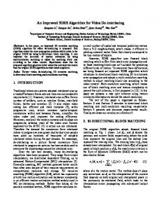
3.1 The algorithm Our algorithm contains two major steps. The first step applies reduction rules to reduce the instance to an irreducible instance and the second step applies branching rules in an irreducible instance to search for a solution. Now we describe a set of branching rules in our algorithm for solving TSP in graphs with maximum degree 4. Note that in our algorithm, there is only one step where F = ∅ may hold. For this case, we simply branch on an arbitrary vertex by including each edge incident on it to F . After this the instance contains some forced edges and we can assume that there always exists some forced vertices. Our branching rules for the case that F ̸= ∅ are given in Figure 1, where for each Case-i, we execute the procedure in Case-i only when there is no vertex v satisfying the condition of Case-j for any j < i. Given an irreducible instance (G, F ̸= ∅), our algorithm first selects an f4-vertex v in (G, F ) if it exists, and branches on an unforced edge e around v (for most cases, the edge e is incident to v). Such a pair of vertex v and edge e is chosen as the one satisfying one of the conditions in Cases-1, 2 and 3 in Figure 1. When there is no f4-vertex in (G, F ), our algorithm selects an f3vertex v in a U -component H that is not a 4-cycle component, and branches on an unforced edge e in H according to Cases-4 to 9 in Figure 1. Recall that any instance such that every U -component is a 4-cycle component is polynomially solvable by Lemma 2. Also see Figure 2 for illustrations for the neighbors of a vertex v in Cases-1 to 9.

8


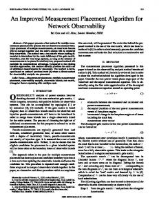
/* while there is an f4-vertex in an irreducible instance (G, F ), choose an f4-vertex v in Cases-1, 2 and 3, where Nu (v) is denoted by {t1 , t2 , t3 } */ Case-1. Nu (v) contains an f4-vertex (say t1 ): (I) if one of t2 and t3 (say t2 ) is joined to a vertex t ∈ Nu (t1 ) − {v} by a chain then branch on edge e = vt3 ; (II) else branch on edge e = vt1 ; Case-2. Nu (v) contains only unforced vertices, where t1 is assumed to be a u3-vertex if Nu (v) contains such a vertex: Branch on edge e = vt1 ; Case-3. Nu (v) contains an f3-vertex (say t1 and let Nu (t1 ) = {v, y1 }): (I) if y1 is a u3-vertex and one of t2 and t3 (say t2 ) is a degree-3 good neighbor of y1 then branch on edge e = y1 z for z ∈ Nu (y1 ) − {t1 , t2 }; (II) else branch on edge e = vt1 ; /* when there is no f4-vertex in an irreducible instance (G, F ), choose an f3-vertex v in Cases-4, 5, 6, 7, 8 and 9, where Nu (v) is denoted by {t1 , t2 } */ Case-4. Nu (v) contains only u3-vertices: Branch on edge e = vt1 ; Case-5. v is in a U -component that is not a 4-cycle component and Nu (v) contains only f3-vertices: Branch on edge e = vt1 ; Case-6. Nu (v) contains a u4-vertex (say t1 ) and an f3-vertex (say t2 ): Branch on edge e = vt1 ; Case-7. Nu (v) contains an f3-vertex (say t1 and let Nu (t1 ) = {v, y1 }) and a u3-vertex (say t2 ), where y1 is a u3-vertex, since now G has no f4-vertices and if y1 is a f3-vertex (resp., u4-vertex) then Case-5 (resp., Case-6) would be applicable to f3-vertex t1 : (I) if y1 ∈ Nu (t2 ) then branch on edge e = y1 z for a good neighbor z (̸= t1 , t2 ) of y1 ; (II) else branch on edge e = vt1 ; Case-8. Nu (v) contains a u4-vertex (say t1 ) and a u3-vertex (say t2 ): (I) if t1 ∈ Nu (t2 ) then branch on edge e = t1 x for a good neighbor x (̸= v, t2 ) of t1 ; (II) else branch on edge e = vt1 ; Case-9. Nu (v) contains only u4-vertices: Branch on edge e = vt1 .

Fig. 1 Branching rules

For an f4-vertex (resp., f3-vertex) v in Figure 1, we always let t1 , t2 and t3 (resp., t1 and t2 ) denote the good neighbors of v, as shown in Figure 2. For each Case-i, we derive branching vectors that evaluate how much the weight decreases in each of the two instances obtained by branching on the selected unforced edge e. In fact, the branching vector for each particular branching operation may not be the finial branching vector for this operation to obtain our results, because we will also use an amortization technique ‘shift’ to save some weight decrease from good branching vectors to bad branching vectors.

3.2 The results To efficiently analyze the search tree of our algorithm, we set∑a vertex weight function ω : V → R+ in the graph and use the sum µ = v∈V (G) ω(v) of the weight of all vertices in the graph as the measure. Since we will require


v

e

e

t3

t2

t1

t3

t2

t1

v

v

v

e

9

t1

t1

t3

t2

t2

x

e t5

t4

v

z

t3

t2

v

v

e

v

e

t1

t1

t2

Case-3(I)

Case-2

Case-1(II)

v

e t1

t5

t4

Case-1(I)

t3

y1

e

t2

t1

t1

t2

t2

y1

e z Case-3(II)

v

Case-6

v

e t1

Case-5

Case-4

t1

t2

Case-7(I)

v t2

v

e t1

e t2

t1

t2

e Case-7(II) : unforced edges

x Case-8(I)

Case-8(II)

Case-9

: forced edges

Fig. 2 Illustration for the branching rules in Case-1 to Case-9

the weight of each vertex to be at most 1, the measure µ is not greater than the number n of vertices. A running time bound related to the measure µ will imply a running time bound related to n. In this paper, we set the vertex weights as follows,  0 for v of degree less than 3;     0 for v in a 4-cycle U -component;    0.45540 for v being a u3-vertex not in a 4-cycle U -component; ω(v) = 0.21968 for v being an f3-vertex not in a 4-cycle U -component;     1 for v being a u4-vertex not in a 4-cycle U -component;    0.59804 for v being an f4-vertex not in a 4-cycle U -component. Lemma 4 With the above vertex weight setting, each branching operation in Figure 1 has an amortized branching factor not greater than 1.69193. We derive a proof of this analytical lemma in the next several sections. From the lemma we get our main result Theorem 1 TSP in an n-vertex graph G with maximum degree 4 can be solved in 1.69193n nO(1) time and polynomial space.

10


4 Weight Decrease To prove Lemma 4, we use the measure-and-conquer method where we ana∑ lyze how much amount of the measure µ = v∈V (G) ω(v) of an instance will decrease after branching operations in our algorithm in Figure 1. We denote w4 = 1, w4′ = 0.59804, w3 = 0.45540 and w3′ = 0.21968.

(2)

In fact, these specific values for weights have been determined by solving a quasiconvex program consisting of the recurrences of our algorithm as constraints. In what follows, we only check that the branching factor of each branching operation in our algorithm does not exceed the time bound in Lemma 4. For notational convenience, we denote ∆4 = w4 −w4′ = 0.40196, ∆3 = w3 − w3′ = 0.23572, ∆4−3 = w4 − w3 = 0.54460 and ∆′4−3 = w4′ − w3′ = 0.37836, where by (2) we have ∆4 ≥ ∆′4−3 ≥ ∆3 ≥ w3′ and ∆4−3 ≥ w3 ≥ ∆′4−3 ≥ 1.5w3′ .

(3)

For an unforced edge uv in an instance (G, F ), define N+ (u, v) = N− (u, v) = {v} if v is a u4-vertex; N+ (u, v) = {v} and N− (u, v) = Nu [v] − {u} if v is a u3-vertex; N+ (u, v) = Nu [v] − {u} and N− (u, v) = {v} if v is an f4-vertex; and N+ (u, v) = N− (u, v) = Nu [v] − {u} if v is an f3-vertex. Thus N+ (u, v) (resp., N− (u, v)) is a set of vertices in Nu [v]−{u} whose weight decreases when uv is added to F (resp., uv is deleted from G) and reductions are applied, and we denote the corresponding weight decrease by ∆+ (u, v) (resp., ∆− (u, v)). See Figure 3. Note that when deleting or forcing an edge to F in an irreducible graph, the weight of each endpoint of the edge increases by at least min{∆4 , ∆3 , ∆4−3 , ∆′4−3 , w3 , w3′ } = w3′ . This is the reason why the weight of the bottom vertex in Figure 3(c), (d), (f) and (h) decreases by at least w3′ . We see that ∆+ (u, v) = ∆4 = 1 − w4′ and ∆− (u, v) = ∆4−3 = 1 − w3 if v is a u4-vertex; ∆+ (u, v) = ∆3 = w3 − w3′ and ∆− (u, v) ≥ w3 + 2w3′ if v is a u3-vertex; ∆+ (u, v) ≥ w4′ + 2w3′ and ∆− (u, v) = ∆′4−3 = w4′ − w3′ if v is an f4-vertex; and ∆+ (u, v) ≥ 2w3′ and ∆− (u, v) ≥ 2w3′ if v is an f3-vertex. We always have ∆+ (u, v) ≥ ∆3

and

∆− (u, v) ≥ ∆′4−3 .

Lemma 5 Let (G, F ) be an instance which consists of u3-, f3-, u4- and f4vertices except for a vertex v, where the degree of v is at most 4 and two forced edges may be incident to v. Let t and t′ be two good neighbors of v such that (a) if t ∈ Nu (t′ ) and one of t and t′ is an f3-vertex then the other of them is not a degree-3 vertex; and (b) if t and t′ are f3-vertices and Nu (t) ∩ Nu (t′ ) − {v} ̸= ∅, then the vertex y ∈ Nu (t) ∩ Nu (t′ ) − {v} = ̸ ∅ is unforced.


force(uv)

∆4=w4-w4’

u

u

u

v

∆3=w3-w3’ v

w4’ v

w3’ (a) u4-vertex v delete(uv)

(b) u3-vertex v

u

∆4-3=w4-w3 v

w3

u w3’

w3’

w3’

(c) f4-vertex v

v

(d) f3-vertex v

u

u

u

v

∆’4-3=w4’-w3’ v

w3’ v

w3’

w3’

(f) u3-vertex v

(g) f4-vertex v (h) f3-vertex v

w3’ (e) u4-vertex v

11

: unforced edges

: newly deleted edges

: forced edges

: newly forced edges

Fig. 3 Illustration for ∆+ (u, v) and ∆− (u, v) for all types of vertex v

Let D denote the weight decrease of vertices in N− (v, t) ∪ N− (v, t′ ) when edges vt and vt′ are deleted during an execution of delete(e) or force(e) for an unforced edge e in (G, F ). Then (i) if neither of t and t′ is an f4-vertex and one of t and t′ is a u3-vertex, then D ≥ w3 + 3w3′ ; (ii) if one of t and t′ is unforced or neither of t and t′ is an f4-vertex, then D ≥ 4w3′ . Proof. (i) Consider the case where one of t and t′ , say t, is a u3-vertex, and neither of t and t′ is an f4-vertex. Let {y1 , y2 } = Nu (t) − {v}. If t′ ̸∈ {y1 , y2 }, then D is at least ∆− (v, t) = w3 +2w3′ plus the weight decrease of t′ , indicating that D ≥ w3 + 3w3′ . Assume that t′ ∈ {y1 , y2 }, say t′ = y1 , where t′ = y1 is unforced, since t′ = y1 is not an f3-vertex by the assumption (a). Hence we still have D ≥ ∆− (v, t) + w3′ = w3 + 3w3′ . (ii) First consider the case where one of t and t′ , say t is unforced. When t is a u3-vertex, D is at least ∆− (v, t) = w3 +2w3′ ≥ 4w3′ . Next, we assume that t is a u4-vertex and t′ is not a u3-vertex. If t ̸∈ N− (v, t′ ), then we have that D ≥ ∆4−3 +∆− (v, t′ ) ≥ ∆4−3 +2w3′ ≥ 4w3′ , where ∆4−3 is the weight decrease of u4-vertex t. The remaining case is that t ∈ N− (v, t′ ), which can happen only when t′ is an f3-vertex and is a good neighbor of t (see Figure 3(e)-(h)). In this case, D is at least the weight decrease of t and t′ ; i.e., D ≥ (w4 − w3′ ) + w3′ ≥ 4w3′ . Next consider the case where neither of t and t′ is an f4-vertex. We can also assume that neither of t and t′ is unforced, since otherwise the above cases can be applied. Then both t and t′ are f3-vertices, where f3-vertex t′ is not a good

12


neighbor of degree-3 vertex t by the assumption (a). Let {y} = Nu (t) − {v} and {y ′ } = Nu (t′ ) − {v}. If y = y ′ , then the vertex y = y ′ is unforced by the assumption (b). Hence deleting edges vt and vt′ and adding edges ty and t′ y ′ to F decrease the weight of vertices y and y ′ (or vertex y = y ′ ). This shows that D ≥ ∆− (v, t) + ∆− (v, t′ ) ≥ 2w3′ + 2w3′ = 4w3′ . ⊔ ⊓ We remark that the assumptions (a) and (b) in the lemma hold when (G, F ) is irreducible as follows. If t ∈ Nu (t′ ) and one of t and t′ , say t′ is a f3-vertex then the other t is not a degree-3 vertex, because otherwise vt′ would be d-reducible. When t and t′ are f3-vertices such that Nu (t)∩Nu (t′ )−{v} = ̸ ∅, the vertex y ∈ Nu (t) ∩ Nu (t′ ) − {v} = ̸ ∅ is unforced, since otherwise the third unforced edge vt′′ incident to v would be d-reducible. In our analysis, the following property is also frequently used. When the first edge in a chain of an irreducible instance is added to F (or deleted from the graph) the other edges in the chain will be alternately deleted from the graph or added to F by Lemma 3(i)-(ii). In the next three sections, we analyze the branching vectors of branching rules in Figure 1.

5 Cases-1, 2 and 3 of Branching on Edges Around f4-vertices This section analyzes the cases of branching on an edge when there is at least one f4-vertex v. We prove that we can branch on edge e in Cases-1, 2 and 3 with a branching vector covered by one of the following: (5w4′ − w3′ ; 2w4′ − 2w3′ );

(4)

(2w4′ + 6w3′ ; 2w4′ − 2w3′ );

(5)

(2w4′ + 6.5w3′ ; 2w4′ − 2w3′ );

(6)

(2 + w4′ − 2w3 + w3′ ; w4′ + 3w3 − 3w3′ );

(7)

(3 − 2w3 ; 1 + w4′ − w3 − w3′ );

(8)

(1 + w4′ − w3 + 5w3′ ; 1); and

(9)

(w4′ + w3 + 7w3′ ; w4′ + w3 − w3′ ).

(10)

In Cases-1, 2 and 3, we let H denote the U -component containing v, and t1 , t2 and t3 denote the good neighbors of v. No two good neighbors ti and tj of v are joined by a chain since otherwise edge vtk with k ̸= i, j would be a bridge and then be d- or f-reducible. We get Proposition 2 In Cases-1, 2 and 3, no two good neighbors ti and tj of v are joined by a chain. In particular, ti and tj are not adjacent via an unforced edge if they are f3-vertices.


13

Case-1. One good neighbor t1 of v is an f4-vertex: We show the next lemma. Lemma 6 Branching on an edge chosen in Case-1 leads to a branching vector covered by at least one of (4), (5) and (6). Let t4 and t5 be the two other good neighbors of t1 than v. Recall that t2 and t3 are not joined by any chain by Proposition 2. For the same reason, t4 and t5 are not joined by any chain either. Case-1 (I). t2 is joined to t4 or t5 (say t5 ) by a chain P : We branch on edge e = vt3 (see Figure 4(a) and (b)). Note that P contains an even number h (≥ 2) of f3-vertices, since otherwise edge vt1 would be d-reducible. We branch on edge e = vt3 . In the branch of force(vt3 ), vt1 , vt2 , t1 t5 and some edges in P will be deleted, and vt3 , t1 t4 and some edges in P will be added to F . Then the weight of t3 and t4 decreases by 2w3′ even if t3 = t4 holds (in this case t3 = t4 is unforced otherwise vt3 is d-reducible because P is a chain containing even number of f3-vertices). In total, force(vt3 ) decreases the weight of vertices in {v, t1 } ∪ V (P ) and {t3 , t4 } (or t3 = t4 ) by at least w4′ + w4′ + hw3′ + 2w3′ = 2w4′ + (h + 2)w3′ , where 2w3′ comes from {t3 , t4 } or t3 = t4 . In the second branch of delete(vt3 ), we delete edges vt3 and t1 t4 , since t1 t4 will be a d-reducible bridge after removal of vt3 . Again the weight of t3 and t4 decreases by 2w3′ even if t3 = t4 . In total this decreases the weight of vertices v, t1 and {t3 , t4 } (or t3 = t4 ) by ∆′4−3 + ∆′4−3 + 2w3′ = 2w4′ . When h = 2, delete(vt3 ) makes H a 4-cycle component, the weight of the four f3-vertices in H will becomes 0, and then the weight of vertices in H further decreases by 4w3′ . In total the measure decreases by at least 2w4′ + 4w3′ in this branch. Hence we get branching vectors: (2w4′ + 6w3′ ; 2w4′ ) for h ≥ 4; and (2w4′ + 4w3′ ; 2w4′ + 4w3′ )

for h = 2,

both of which are covered by (4) (i.e., (5w4′ − w3′ ; 2w4′ − 2w3′ )), since for (a; b) ∈ {(2w4′ + 6w3′ ; 2w4′ ), (2w4′ + 4w3′ ; 2w4′ + 4w3′ )} and (a′ ; b′ ) = (5w4′ − w3′ ; 2w4′ − 2w3′ ), we have a + b ≥ a′ + b′ and b ≥ b′ . Case-1 (II). No vertex ti ∈ {t2 , t3 } is joined to any vertex in {t4 , t5 } by a chain: We branch on edge e = vt1 (see Figure 4(c) and (d)). Recall that t2 and t3 (resp., t4 and t5 ) are not joined by any chain. In the branch of delete(vt1 ), the weight of v and t1 decreases by 2∆′4−3 = 2w4′ − 2w3′ . In what follows, we consider the measure decrease in the branch of force(vt1 ). For convenience, let T = {t2 , t3 , t4 , t5 }, and denote (v ′ , ti ) = (v, ti ) for i = 2, 3 and (v ′ , ti ) = (t1 , ti ) for i = 4, 5. Now no two vertices in T are joined by a chain. We distinguish three subcases (i)-(iii). Case-1 (II-i) {t2 , t3 } ∩ {t4 , t5 } = ∅: In the branch of force(vt1 ), we also delete edges vt2 , vt3 , t1 t4 and t1 t5 from G, decreasing the weight of vertices v

14


w4’ w4’

v

∆’4-3

e

t1

w3’

w3’

t5

t1

w3’

t5

4

(b) delete(vt3) in Case-1(I)

v

∆’4-3

e w4’

t3

t2

P w3’ t

(a) force(vt3) in Case-1(I)

w4’

e

t ∆’4-3 1

w3’

P w3’ t4

t3

t2

v

v

e t2

t3

∆’4-3

t1

t2

t3

2w3 w3’

t 4 t5 (c) force(vt1) in Case-1(II)

(d) delete(vt1) in Case-1(II)

: unforced edges


: forced edges


Fig. 4 Illustration for Case-1, where v is an f4-vertex such that one of ti , say t1 is an f4-vertex

and t1 by w4′ + w4′ . We claim that this branch decreases the weight of other vertices in V − {v, t1 } by at least 6w3′ when T consists only of f4-vertices; and 6.5w3′ otherwise. In the branch of force(vt1 ), the weight of a non-f3-vertex ti ∈ T (resp., an f3-vertex ti ∈ T ) decreases by at least min{∆4−3 , w3 , ∆′4−3 } = ∆′4−3 (resp., by at least w3′ ). For each f3-vertex ti ∈ T , we have ∆− (v ′ , ti ) ≥ 2w3′ . Note that v, t1 ̸∈ ∆− (v ′ , ti ) since {t2 , t3 } ∩ {t4 , t5 } = ∅. To prove the claim, we consider three cases (a)-(e). (a) T contains no f3-vertex: Then the branch of force(vt1 ) decreases the weight of the vertices in T by at least 4∆′4−3 , which is at least 6w3′ by (3). If T contains a non-f4-vertex, then the branch of force(vt1 ) decreases the weight of the vertices in T by at least 3∆′4−3 + min{∆4−3 , w3 } (≥ 6.5w3′ by (2) and (3)). (b) T contains exactly one f3-vertex, say t2 : If N− (v, t2 ) ∩ (T − {t2 }) = ∅, then the branch of force(vt1 ) decreases the weight of the vertices in T ∪ N− (v, t2 ) by at least 3∆′4−3 + 2w3′ (≥ 6.5w3′ by (3)). Assume that there is a vertex tj ∈ N− (v, t2 ) ∩ (T − {t2 }). Then tj is not an f3-vertex since no chain connects t2 and tj . If tj is an f4-vertex or u4-vertex,


15

then the branch of force(vt1 ) decreases the weight of the vertices in T by at least 2∆′4−3 + w3′ + min{w4 − w3′ , w4′ } (≥ 6.5w3′ by (2) and (3)). If tj is a u3-vertex, then the branch of force(vt1 ) decreases the weight of the vertices in T and the good neighbor z (̸= v, ti ) of tj (possibly z ∈ T − {ti , tj }) by at least 2∆′4−3 + w3′ + w3 + w3′ (≥ 7w3′ by (3)). (c) T contains at least two f3-vertices ti and tj in T that have a common good neighbor z ∈ N− (v ′ , ti ) ∩ N− (v ′ , tj ): We see that z is unforced, since otherwise vt1 would be d-reducible. If z = tk for some tk ∈ T − {ti , tj }, then z = tk must be a u4-vertex and z has a good neighbor x ̸∈ {v, t1 } ∪ T (otherwise a bridge of the U component containing v would appear at vertex th ∈ T − {ti , tj , tk }), and the branch of force(vt1 ) decreases the weight of vertices in T ∪ {z, x} by at least 3w3′ + w4 + w3′ (≥ 6.5w3′ by (2) and (3)). Assume that z ̸∈ T , and let x (̸= ti , tj ) be a good neighbor of z, where in the branch of force(vt1 ) the weight of x decreases by at least w3 if x ∈ T (resp., by at least w3′ if x ̸∈ T ). Hence the branch of force(vt1 ) decreases the weight of vertices in T − {ti , tj } and (N− (v ′ , ti ) ∩ N− (v ′ , tj )) ∪ {x} by at least w3′ + w3 + 2w3′ + w3 (when x ∈ T ) or 2w3′ + 3w3′ + w3 (when x ̸∈ T ), where min{w3′ + w3 + 2w3′ + w3 , 2w3′ + 3w3′ + w3 } ≥ 7w3′ by (3). (d) T contains at least two f3-vertices ti and tj each of which is not a good neighbor of a vertex in T and T − {ti , tj } contains a non-f3-vertex: Assume that ti and tj have no common good neighbor, otherwise we can apply case (c). Then the branch of force(vt1 ) decreases the weight of the vertices in T by at least w3′ + ∆′4−3 + 4w3′ (≥ 6.5w3′ by (3)). Note that the case where T contains three f3-vertices is covered by (c) and (d). (e) T contains only f3-vertices: Analogously with (c), no two vertices in T are adjacent by an unforced edge. Also no three vertices in T have a common good neighbor since otherwise vt1 would be d-reducible. When some pair of vertices in T have a common good neighbor, we assume that ti and tj (resp., tk and th ) have a common good neighbor for {i, j, k, h} = {2, 3, 4, 5} without loss of generality. As observed in (c), any common good neighbor of ti and tj is unforced. Then the branch of force(vt1 ) decreases the weight of vertices in N− (v ′ , ti ) ∪ N− (v ′ , tj ) by at least 2w3′ + min{2w3′ , w3 } (≥ 4w3′ ). Similarly for N− (v ′ , tk ) ∪ N− (v ′ , th ). In total the branch of force(vt1 ) decreases the weight of T and its good neighbors by at least 8w3′ . The above Cases (a)-(e) prove that the branch of force(vt1 ) decreases the measure by at least 2w4′ + 6w3′ (resp., by 2w4′ + 6.5w3′ when T contains a non-f4-vertex). Hence we have branching vectors (2w4′ + 6w3′ ; 2w4′ − 2w3′ ); i.e., (5); and (2w4′ + 6.5w3′ ; 2w4′ − 2w3′ ); i.e., (6) for the case where T contains a non-f4-vertex, which will be used for saving a shift σ2 for branching vector (8) in Case-2(ii).

16


Case-1 (II-ii) |{t2 , t3 } ∩ {t4 , t5 }| = 1: Let t2 = t4 , which is a degree-4 vertex, since otherwise vt1 would be d-reducible. Let z2 be a good neighbor of t2 different from v and t1 . In the branch of force(vt1 ), edges vt1 and t2 z2 are added to F , and edges vt2 , vt3 , t1 t2 and t1 t5 are deleted. We will show that force(vt1 ) decreases the weight of vertices in {v, t1 } ∪ Nu [t2 ] ∪ N− (v ′ , t3 ) ∪ N− (v ′ , t5 ) by at least 5w4′ − w3′ to obtain the following branching vector (5w4′ − w3′ ; 2w4′ − 2w3′ ), i.e., (4). To finish the proof, we consider three cases (a)-(c). (a) t2 = t4 is a u4-vertex and z2 ̸∈ {t3 , t5 }: force(vt1 ) decreases the weight of vertices in {v, t1 , t2 = t4 , t3 , t5 , z2 } by at least w4′ +w4′ +w4 +w3′ +w3′ +w3′ , which is at least 5w4′ − w3′ by (2). (b) t2 = t4 is a u4-vertex or an f4-vertex and z2 ∈ {t3 , t5 }, say z2 = t3 : Now z2 is a degree-4 vertex, since if z2 = t3 is an f3-vertex then t1 t5 would be a bridge, and if z2 = t3 is a u3-vertex, then vt2 would be d-reducible. Let z3 be a good neighbor of z2 = t3 other than v and t2 = t4 . The branch of force(vt1 ) decreases the weight of vertices in {v, t1 , t2 = t4 } by at least w4′ + w4′ + w4′ = 3w4′ . It suffices to show that the branch of force(vt1 ) decreases the weight of other vertices by at least 2w4′ − w3′ . When z2 = t3 is a u4-vertex, in the branch of force(vt1 ), z2 = t3 will become an f3-vertex at least and the weight of vertices in {z2 = t3 , t5 } decreases by at least (w4 −w3′ )+w3′ , which is at least 2w4′ −w3′ by (2). Next we assume that z2 = t3 is an f4-vertex. If z3 ̸= t5 , then force(vt1 ) decreases the weight of z2 = t3 , t5 and z3 by at least w4′ + w3′ + w3′ (≥ 2w4′ − w3′ by (2)). Let z3 = t5 . Then z3 = t5 is a u4-vertex since otherwise the U -component H containing v would have a bridge or take an odd value in |∂f (H)| Hence force(vt1 ) decreases the weight of t3 and t5 by w4′ + w4 (≥ 2w4′ − w3′ by (2)). (c) t2 = t4 is an f4-vertex and z2 ̸∈ {t3 , t5 }: the branch of force(vt1 ) decreases the weight of vertices in {v, t1 , t2 = t4 } by 3w4′ . It suffices to show that the branch of force(vt1 ) deceases the weight of other vertices by at least 2w4′ − w3′ . In the branch of force(vt1 ), if vertex ti with i = 3, 5 is not an f3-vertex, then the weight of ti decreases by at least ∆′4−3 ; and if vertex ti with i = 3, 5 is an f3-vertex, then the weight of vertices in N− (v ′ , ti ) decreases by at least 2w3′ . In the latter, if z2 ∈ N− (v ′ , ti ), then z2 is not an f3-vertex since otherwise the U -component H containing v would have a bridge, and thereby the weight of vertices in N− (v ′ , ti ) decreases by at least w3′ + w3 . If at most one of t3 and t5 is an f3-vertex, then force(vt1 ) decreases the weight of vertices in N− (v ′ , t3 )∪N− (v ′ , t5 )∪{z2 } by at least ∆′4−3 +min{∆′4−3 + w3′ , 2w3′ + w3′ , w3′ + w3 } = 2w4′ − w3′ . Next we assume that both of t3 and t5 are f3-vertices. It is impossible that t3 and t5 are jointed by a chain since otherwise the U -component H containing v would have a bridge t2 z2 . Hence t3 is not a good neighbor of t5 and shares no common neighbor of an f3-vertex with t5 . If N− (v ′ , t3 ) ∩ N− (v ′ , t5 ) = ∅, then force(vt1 ) decreases the weight of vertices in N− (v ′ , t3 )∪N− (v ′ , t5 )∪{z2 } by at least 2w3′ +2w3′ +w3′ (when z2 ̸∈


17

N− (v ′ , t3 ) ∪ N− (v ′ , t5 )) and by at least 2w3′ + w3′ + w3 (when z2 ∈ N− (v ′ , ti ) for i = 3 or 5), where 2w3′ + w3′ + w3 ≥ 2w3′ + 2w3′ + w3′ ≥ 2w4′ − w3′ . Assume that N− (v ′ , t3 ) ∩ N− (v ′ , t5 ) ̸= ∅. Then t3 and t5 have a common good neighbor z5 , which is not an f3-vertex. If z5 = z2 then z5 is a degree4 vertex since otherwise the U -component H containing v would have an odd value in |∂f (H)|. Then force(vt1 ) decreases the weight of vertices in N− (v ′ , t3 )∪N− (v ′ , t5 )∪{z2 } by at least 2w3′ +w3 +w3′ (when z5 ̸= z2 ) and by at least 2w3′ +w4′ (when z5 = z2 ), where 2w3′ +w3 +w3′ ≥ 2w3′ +w4′ ≥ 2w4′ −w3′ . by (2) and (3). Case-1 (II-iii) {t2 , t3 } = {t4 , t5 } (say t2 = t4 and t3 = t5 ): As in (ii), each vertex in {t2 , t3 } = {t4 , t5 } is of degree 4. In the branch of force(vt1 ), vt2 , vt3 , t1 t2 and t1 t3 are deleted, and vt1 and all other unforced edges incident to t2 or t3 are added to F . We consider two cases (a) and (b). (a) one of t2 and t3 is a u4-vertex or t2 is not a good neighbor of t3 : If one of t2 and t3 , say t2 is a u4-vertex, then in the branch of force(vt1 ) the weight of t2 and a good neighbor z2 ∈ Nu (t2 ) − {v, t1 , t2 , t3 } decreases by at least w4 + w3′ and then the weight of vertices v, t1 , t2 , z2 and t3 decreases by at least w4′ + w4′ + w4 + w3′ + w4′ (≥ 4w4′ + 2w3′ by (2)). Assume that both t2 and t3 are f4-vertices. Since t2 is not a good neighbor of t3 , t2 and t3 have good neighbors z2 ∈ Nu (t2 ) − {v, t1 , t2 , t3 } and z3 ∈ Nu (t3 ) − {v, t1 , t2 , t3 }, and force(vt1 ) decreases the weight of vertices v, t1 , t2 , z2 , t3 and z3 by at least w4′ + w4′ + w4′ + w3′ + w4′ + w3′ = 4w4′ + 2w3′ (even if z2 = z3 since in this case z2 = z3 is unforced). Hence we have branching vector (4w4′ + 2w3′ ; 2w4′ − 2w3′ ), which is covered by (4) (i.e., (5w4′ − w3′ ; 2w4′ − 2w3′ )), since for (a; b) = (4w4′ + 2w3′ ; 2w4′ − 2w3′ ) and (a′ ; b′ ) = (5w4′ − w3′ ; 2w4′ − 2w3′ ), we have a + b ≥ a′ + b′ and b ≥ b′ . (b) t2 and t3 are f4-vertices, and t2 is a good neighbor of t3 : In this case, force(vt1 ) decreases the weight of vertices v, t1 , t2 and t3 by 4w4′ . In the other branch of delete(vt1 ), we remove edge t2 t3 since it becomes d-reducible and the U -component with {v, t1 , t2 , t3 } becomes a 4-cycle component, decreasing the measure by 4w4′ . Hence we have branching vector (4w4′ ; 4w4′ ), which is covered by (4) (i.e., (5w4′ − w3′ ; 2w4′ − 2w3′ )), since for (a; b) = (4w4′ ; 4w4′ ) and (a′ ; b′ ) = (5w4′ − w3′ ; 2w4′ − 2w3′ ), we have a + b ≥ a′ + b′ and b ≥ b′ . Case-2. Nu (v) contains only unforced vertices, where t1 is assumed to be a u3-vertex if Nu (v) contains such a vertex: We branch on edge e = vt1 . We show the next lemma. Lemma 7 Branching on an edge e = vt1 chosen in Case-2 leads to a branching vector covered by (7) or (8).

18


To prove the lemma, we distinguish two subcases (i) and (ii) in Case-2. Case-2(i) Nu (v) contains only u4-vertices: See Figure 5(a) and (b). In the branch of delete(vt1 ), the weight of vertices v and t1 decreases by ∆′4−3 + ∆4−3 = 1 + w4′ − w3 − w3′ . In the branch of force(vt1 ), edge vt1 will be added to F and edges vt2 and vt3 will be deleted, where we denote the resulting instance (G1 , F1 ). In (G1 , F1 ), the weight of vertices v, t1 , t2 and t3 decreases by w4′ + ∆4 + ∆4−3 + ∆4−3 = 3 − 2w3 . We call an executing force(vt1 ) basic if force(vt1 ) decreases the measure by only 3 − 2w3 before an irreducible instance (G′ , F ′ ) is obtained. We consider two cases (a) and (b).

w4’

v

∆’4-3

e t1 ∆4

t2 ∆4-3

∆4-3

t3

t1 ∆4-3

(a) force(vt1) in Case-2(i)

w4’

∆’4-3

e t2 ∆4-3

∆4-3

z1

t2

t3

z2

(c) force(vt1) in Case-2(ii)

t3

(b) delete(vt1) in Case-2(i)

v

t1 ∆3

v

e

w3 y1 ∆3

t1

v

e t2

t3

y2 ∆3 (d) delete(vt1) in Case-2(ii)

: unforced edges


: forced edges


Fig. 5 Illustration for Case-2, where v is an f4-vertex such that Nu (v) contains only unforced vertices, where t1 is assumed to be a u3-vertex if Nu (v) contains such a vertex

(a) An execution of force(vt1 ) is basic; i.e., (G1 , F1 ) = (G′ , F ′ ): As observed in the above, we obtain a branching vector (3 − 2w3 ; 1 + w4′ − w3 − w3′ ); i.e., (8). We here analyze the structure of the resulting irreducible instance (G′ , F ′ ) after the basic execution of force(vt1 ). No other unforced edge than vt1 , vt2 and vt3 is deleted or added to F during force(vt1 ), and hence t1 will be an f4-vertex in (G′ , F ′ ). Recall that in Case-2 no two f4-vertices are adjacent by


19

an unforced edge in (G, F ). Hence in (G′ , F ′ ), any unforced edge between two f4-vertices must be incident to t1 . Therefore the resulting irreducible instance (G′ , F ′ ) has a structure that if an f4-vertex v has an f4-vertex t as a good neighbor, then v or t has a non-f4-vertex among their neighbors. (b) An execution of force(vt1 ) is not basic; i.e., (G1 , F1 ) ̸= (G′ , F ′ ): Note that vertices t2 and t3 are u3-vertice in (G1 , F1 ). Then one of the following holds in (G1 , F1 ): (i) A reduction is applied so that at least one unforced edge is added to F or deleted, which decreases the weight of the two endpoints of the edge by at least 2 min{∆4 , ∆3 , ∆4−3 , ∆′4−3 , w3 , w3′ } = 2w3′ ; and (ii) the reduction in Lemma 3(iv) is applied, which decreases the measure by at least 2w3′ . Therefore, force(vt1 ) decreases the measure of (G, F ) by at least 3 − 2w3 + 2w3′ , indicating a branching vector (3 − 2w3 + 2w3′ ; 1 + w4′ − w3 − w3′ ), which is covered by (7) (i.e., (2 + w4′ − 2w3 + w3′ ; w4′ + 3w3 − 3w3′ )), since for (a; b) = (3 − 2w3 + 2w3′ ; 1 + w4′ − w3 − w3′ ) and (a′ ; b′ ) = (2 + w4′ − 2w3 + w3′ ; w4′ + 3w3 − 3w3′ ), we have a + b ≥ a′ + b′ and b ≥ b′ by (2). Case-2(ii) t1 is a u3-vertex: See Figure 5(c) and (d). Let y1 and y2 be the two good neighbors in Nu (t1 ) − {v}. We first show that the branch of delete(vt1 ) decreases the weight of vertices v and t1 by ∆′4−3 + w3 (= w4′ − w3′ + w3 ) and that of some other vertices by at least 2w3 − 2w3′ , in total by at least w4′ + 3w3 − 3w3′ . If one of y1 and y2 is an f4-vertex, then the branch of delete(vt1 ) decreases the weight of the f4-vertex and vertices t2 and t3 by at least w4′ + w3′ + w3′ (> 2w3 − 2w3′ ), as required. Assume that neither of y1 and y2 is an f4-vertex. For each i = 1, 2, the branch of delete(vt1 ) decreases the weight of vertices in N+ (t1 , yi ) by ∆+ (t1 , yi ) ≥ 2w3′ (≥ w3 − w3′ ) if yi is an f3-vertex, and by ∆+ (t1 , yi ) ≥ min{∆4 , ∆3 , w4′ + 2w3′ } = ∆3 = w3 − w3′ otherwise. Then if N+ (t1 , y1 ) ∩ N+ (t1 , y2 ) = ∅, then the branch of delete(vt1 ) decreases the weight of vertices in N+ (t1 , y1 )∪N+ (t1 , y2 ) by at least (w3 −w3′ )+(w3 −w3′ ) = 2w3 − 2w3′ , as required. Assume that N+ (t1 , y1 ) ∩ N+ (t1 , y2 ) ̸= ∅. This is possible only when both y1 and y2 are f3-vertices, since neither of y1 and y2 is an f4-vertex. Also f3-vertices y1 and y2 are not joined by an unforced edge since otherwise t1 y1 y2 would be a reducible triangle. Then there is a vertex x ∈ N+ (t1 , y1 ) ∩ N+ (t1 , y2 ) − {y1 , y2 }, which must be a degree-4 vertex, since otherwise vt1 would be f-reducible. Hence the branch of delete(vt1 ) still decreases the weight of vertices in N+ (t1 , y1 ) ∪ N+ (t1 , y2 ) by at least 2(w3 − w3′ ), as required. Next we show that the other branch of force(vt1 ) decreases the measure of (G, F ) by at least 2 + w4′ − 2w3 + w3′ to obtain a branching vector (2 + w4′ − 2w3 + w3′ ; w4′ + 3w3 − 3w3′ ); i.e., (7). If both t2 and t3 are u4-vertices, then the branch of force(vt1 ) decreases the weight of vertices v, t1 , t2 and t3 by at least w4′ + ∆3 + ∆4−3 + ∆4−3 = 2+w4′ −w3 −w3′ ≥ 2+w4′ −2w3 +w3′ , as required. Assume that one of t2 and

20


t3 (say t2 ) is a u3-vertex, and let {z1 , z2 } = Nu (t2 ) − {v}. By Proposition 1, t1 ̸∈ {z1 , z2 }, and zi = t3 holds for some i = 1, 2 only when t3 is a u4vertex, where if zi = t3 holds for some i = 1, 2 then let z2 = t3 . Hence the branch of force(vt1 ) decreases the weight of vertices v, t1 , t2 , t3 and z1 by w4′ + w3 + ∆3 + min{∆4−3 , w3 } + w3′ = w4′ + 3w3 (by ∆4−3 ≥ w3 ) and the weight of z2 by at least w3′ (even if z2 is equal to the u4-vertex t3 ). In total, the branch of force(vt1 ) decreases the measure by at least w4′ + 3w3 + w3′ , which is at least 2 + w4′ − 2w3 + w3′ by (2). Case-3. t1 is an f3-vertex, and neither of t2 and t3 is an f4-vertex: We show the next lemma. Lemma 8 Branching on an edge chosen in Case-3 leads to a branching vector covered by (9) or (10). Let y1 be the good neighbor of t1 other than v. When ti (i = 2, 3) is an f3-vertex, let yi denote the good neighbor of ti other than v. Case-3 (I) y1 is a u3-vertex, and one of t2 and t3 (say t2 ) is a degree-3 good neighbor of y1 (where t2 is an f3- or u3-vertex): See Figure 2. Note that y1 ̸∈ {t2 , t3 }, since otherwise edge vt1 would be d-reducible. Let x be the neighbor of t2 other than y1 and v, where possibly t2 x ∈ F . We branch on edge e = y1 z for z ∈ Nu (y1 )−{t1 , t2 }. In the branch of force(y1 z), edge y1 z will be added to F , and edge vt3 will be deleted, where edge t2 x will be added to F if t2 x ̸∈ F . This makes vt1 y1 t2 a 4-cycle U -component changing the weight of each vertex in it to 0. Then the branch of force(y1 z) decreases the weight of vertices in {v, t1 , t2 , t3 , y1 , z} by at least w4′ +w3′ +w3′ +w3′ +w3 +w3′ = w4′ +w3 +4w3′ . In the other branch of delete(y1 z), edges y1 z and vt1 will be deleted, and edges t1 y1 and t2 y1 will be added to F , decreasing the weight of vertices in {v, t1 , t2 , y1 , z} by at least ∆′4−3 + w3′ + w3′ + w3 + w3′ = w4′ + w3 + 2w3′ . Hence we obtain a branching vector (w4′ + w3 + 4w3′ ; w4′ + w3 + 2w3′ ), which is covered by (9) (i.e., (1 + w4′ − w3 + 5w3′ ; 1)), since for (a; b) = (w4′ + w3 + 4w3′ ; w4′ + w3 + 2w3′ ) and (a′ ; b′ ) = (1 + w4′ − w3 + 5w3′ ; 1), we have a + b ≥ a′ + b′ and b ≥ b′ by(2). Case-3 (II) y1 is not a u3-vertex, or neither of t2 and t3 is a degree-3 good neighbor of y1 : We branch on edge e = vt1 . We distinguish cases (i)-(iv) in Case-3 (II) according to the vertex-type of y1 . Case-3 (II-i) y1 is an f4-vertex (see Figure 6(a) and (b)): Note that y1 ̸∈ {t2 , t3 } because neither of t2 and t3 is an f4-vertex. Let {z1 , z2 } = Nu (y1 )−{t1 }, where neither of z1 and z2 is an f4-vertex since Case-1 is no longer applicable. In the branch of force(vt1 ), after including vt1 to F and deleting t1 y1 , the weight of vertices v, t1 and y1 decreases by w4′ + w3′ + ∆′4−3 = 2w4′ and y1 becomes an f3-vertex. Let (G′ , F ′ ) be the instance obtained from (G, F ) by adding edge vt1 to F and deleting edge t1 y1 from G, where we regard the two forced edges incident to the new degree-2 vertex t1 as a singe forced edge ignoring the vertex


21

t1 . In the branch of force(vt1 ), edges vt2 and vt3 will be further deleted from (G′ , F ′ ) and reductions will be applied. Since (G, F ) is irreducible, we see that vertices t2 and t3 in (G′ , F ′ ) satisfy the conditions in Lemma 5. Hence after the branch of force(vt1 ), the weight of vertices in N− (v, t2 ) ∪ N− (v, t3 ) decreases by 4w3′ by Lemma 5. In total, force(vt1 ) decreases the weight of vertices in {v, t1 , y1 } ∪ N− (v, t2 ) ∪ N− (v, t3 ) by at least 2w4′ + 4w3′ . In the other branch of delete(vt1 ), the weight of vertices in {v, t1 , y1 } ∪ N− (y1 , z1 ) ∪ N− (y1 , z2 ) decreases by ∆′4−3 + w3′ + w4′ + 4w3′ = 2w4′ + 4w3′ by applying Lemma 5 to the instance (G′′ , F ′′ ) obtained from (G, F ) by deleting edge vt1 , adding edge t1 y1 and regarding the two forced edges incident to t1 as a single forced edge. Hence we obtain a branching vector (2w4′ + 4w3′ ; 2w4′ + 4w3′ ), which is covered by (9) (i.e., (1 + w4′ − w3 + 5w3′ ; 1)), since for (a; b) = (2w4′ + 4w3′ ; 2w4′ + 4w3′ ) and (a′ ; b′ ) = (1 + w4′ − w3 + 5w3′ ; 1), we have a + b ≥ a′ + b′ and b ≥ b′ by (2).

w4’ v

∆’4-3

w3’

t1

t3

t2 ∆3

w3’

t1

t2 y1

w4’ ∆3

(a) force(vt1) in Case-3(II-i)

z1

z2

∆’4-3

v

e

e t1

t2 w3

t3

w3’

t1

t2

t3

∆3

w3’ y1 ∆3

∆3

(b) delete(vt1) in Case-3(II-i)

w4’ v w3’

t3

∆3

y1

∆’4-3

v

e

e

w3’ y1 z1

∆3

(c) force(vt1) in Case-3(II-ii)

z1

(d) delete(vt1) in Case-3(II-ii)

: unforced edges


: forced edges


Fig. 6 Illustration for Case-3 (II-i) and (II-ii), where v is an f4-vertex such that one of ti , say t1 is an f3-vertex

22


Case-3 (II-ii) y1 is an f3-vertex (see Figure 6(c) and (d)): Let {z1 } = Nu (y1 ) − {t1 }. Note that y1 ̸= t2 , t3 and then N− (y1 , z1 ) ∩ {v, t1 , y1 } = ∅, because no two forced degree-3 vertices in Nu (v) are adjacent by an unforced edge by Proposition 2. In the branch of delete(vt1 ), the weight of vertices v, t1 , y1 and N− (y1 , z1 ) decreases by ∆′4−3 + w3′ + w3′ + ∆′4−3 = 2w4′ . We show that the other branch of force(vt1 ) decreases the measure by at least w4′ +7w3′ . Note that if z1 = ti for some i = 2, 3 then ti is a u4-vertex, since if z1 = ti is an f3-vertex (resp., u3-vertex) then edge vtj with j ∈ {2, 3} − {i} would be d-reducible (resp., edge ti x for x ∈ Nu (ti )−{v} would be f-reducible). In the branch of force(vt1 ), the weight of vertices in N− (v, t2 ) ∪ N− (v, t3 ) decreases by at least 4w3′ by Lemma 5. In particular, when one of t2 and t3 is a u3-vertex, then the weight of vertices in N− (v, t2 ) ∪ N− (v, t3 ) decreases by at least w3 + 3w3′ ≥ 5w3′ by Lemma 5. Hence if one of t2 and t3 is a u3-vertex, then force(vt1 ) decreases the weight of vertices in {v, t1 , y1 } ∪ N− (v, t2 ) ∪ N− (v, t3 ) by at least w4′ + w3′ + w3′ + (w3 + 3w3′ ) ≥ w4′ + 7w3′ , as required. We assume that none of t2 and t3 is a u3-vertex. If z1 ̸∈ N− (v, t2 ) ∪ N− (v, t3 ), then force(vt1 ) decreases the weight of vertices in {v, t1 , y1 , z1 } ∪ N− (v, t2 ) ∪ N− (v, t3 ) by at least w4′ + 3w3′ + 4w3′ = w4′ + 7w3′ , as required. If z1 ∈ {t2 , t3 }, then force(vt1 ) decreases the weight of vertices in {v, t1 , y1 , t2 , t3 } by at least w4′ +w3′ +w3′ +w4 +w3′ = w4′ +3w3′ +1 ≥ w4′ +7w3′ , as required. Next assume that z1 ∈ N− (v, t2 ) ∪ N− (v, t3 ) − {t2 , t3 }; i.e., z1 is a good neighbor of an f3-vertex t2 or t3 , say z1 ∈ Nu (t2 ). Then z1 is an unforced vertex (otherwise vt1 would be f-reducible). If z1 is also a good neighbor of t3 , then t3 is a u4-vertex (since if t3 ∈ Nu (t2 ) ∩ Nu (t3 ) is an f3-vertex, then the U -component H containing v would have a bridge at z1 or take an odd value in |∂f (H)|). Hence force(vt1 ) decreases the weight of vertices in {v, t1 , y1 , z1 , t2 }∪ N− (v, t3 ) by at least w4′ +w3′ +w3′ +w3 +w3′ +2w3′ ≥ w4′ +7w3′ , as required. Hence we obtain a branching vector (w4′ + 7w3′ ; 2w4′ ), which is covered by (9) (i.e., (1 + w4′ − w3 + 5w3′ ; 1)), since for (a; b) = (w4′ + 7w3′ ; 2w4′ ) and (a′ ; b′ ) = (1 + w4′ − w3 + 5w3′ ; 1), we have a + b ≥ a′ + b′ and b ≥ b′ by (2). Case-3 (II-iii) y1 is a u4-vertex (see Figure 7(a) and (b)): In the branch of delete(vt1 ), the weight of vertices v, t1 and y1 decreases by ∆′4−3 + w3′ + ∆4 = 1. In what follows, we show that the branch of force(vt1 ) decreases the measure by at least 1 + w4′ − w3 + 5w3′ to obtain a branching vector (1 + w4′ − w3 + 5w3′ ; 1); i.e., (9). First consider the case that y1 ∈ {t2 , t3 } (say y1 = t2 ). Since t2 = y1 is a u4-vertex, there is a good neighbor z of t2 which is not in {v, t1 , t2 , t3 }. Then the branch of force(vt1 ) decreases the weight of vertices v, t1 , y1 = t2 , t3 and z by w4′ + w3′ + w4 + w3′ + w3′ , which is at least 1 + w4′ − w3 + 5w3′ by (2).


w4’ v

∆’4-3

t1

t2 w3

y1

∆4-3

t3

w3’

t1

t2

∆4

y1

(b) delete(vt1) in Case-3(II-iii)

w4’ v

∆’4-3

t2 w3

t3

w3’

t1

t2

t3

w3

w3 y1 ∆3

v

e

e t1

t3

w3

(a) force(vt1) in Case-3(II-iii)

w3’

v

e

e w3’

23

∆3

y1

z1 ∆ z2 3 (c) force(vt1) in Case-3(II-iv)

(d) delete(vt1) in Case-3(II-iv)

: unforced edges


: forced edges


Fig. 7 Illustration for Case-3 (II-iii) and (II-iv), where v is an f4-vertex such that one of ti , say t1 is an f3-vertex

Next consider the case that y1 ̸∈ {t2 , t3 }. Let (G′ , F ′ ) be the instance obtained from (G, F ) by adding edge vt1 to F and deleting edge t1 y1 from G, where we regard the two forced edges incident to the new degree-2 vertex t1 as a singe forced edge ignoring the vertex t1 . In the branch of force(vt1 ), edges vt2 and vt3 will be further deleted from (G′ , F ′ ) and reductions will be applied. Since (G, F ) is irreducible, we see that vertices t2 and t3 in (G′ , F ′ ) satisfy the conditions in Lemma 5. Hence after the branch of force(vt1 ), the weight of vertices in N− (v, t2 ) ∪ N− (v, t3 ) decreases by 4w3′ by Lemma 5. In total, force(vt1 ) decreases the weight of vertices in {v, t1 , y1 } ∪ N− (v, t2 ) ∪ N− (v, t3 ) by at least w4′ + w3′ + ∆4−3 + 4w3′ = 1 + w4′ − w3 + 5w3′ . Case-3 (II-iv) y1 is a u3-vertex, and neither of t2 and t3 is a degree3 good neighbor of y1 (see Figure 7(c) and (d)): Note that y1 ̸∈ {t2 , t3 }, since otherwise edge vt1 would be d-reducible. Let {z1 , z2 } = Nu (y1 ) − {t1 }. Note that if zi ∈ {t2 , t3 } then zi is a u4-vertex since if it is of degree 3 then the condition of Case-3 (II-i) would hold (recall that no good neighbor of v is an f4-vertex since Case-1 is not applicable). We branch on edge vt1 . In the branch of delete(vt1 ), the weight of vertices v, t1 and y1 decreases by ∆′4−3 + w3′ + ∆3 = w4′ + w3 − w3′ . Next we analyze the branch of force(vt1 ).

24


If {z1 , z2 } ∩ {t2 , t3 } ̸= ∅, then force(vt1 ) decreases the weight of vertices in {v, t1 , y1 , z1 , z2 } ∪ {t2 , t3 } by at least w4′ + w3′ + w3 + w3′ + 1 + w3′ ≥ w4′ + w3 + 7w3′ (when |{z1 , z2 } ∩ {t2 , t3 }| = 1) or by at least w4′ + w3′ + w3 + 1 + 1 ≥ w4′ + w3 + 7w3′ (when |{z1 , z2 } ∩ {t2 , t3 }| = 2). If {z1 , z2 }∩(N− (v, t2 )∪N− (v, t3 )) = ∅, then {v, t1 , y1 , z1 , z2 }∩(N− (v, t2 )∪ N− (v, t3 )) = ∅. In the branch of force(vt1 ), the weight of vertices in N− (v, t2 )∪ N− (v, t3 ) decreases by 4w3′ by Lemma 5. In total force(vt1 ) decreases the weight of vertices in {v, t1 , y1 , z1 , z2 } ∪ N− (v, t2 ) ∪ N− (v, t3 ) by at least w4′ + w3′ + w3 + 2w3′ + 4w3′ = w4′ + w3 + 7w3′ . The remaining case is that zi ∈ N− (v, t2 ) ∪ N− (v, t3 ) − {t2 , t3 } for some i = 1, 2, where zi is not a forced vertex, since otherwise vt1 would be dreducible. We see that, for each i = 1, 2 vertex zi cannot be in N− (v, t2 ) ∩ N− (v, t3 ) − {t2 , t3 }, since otherwise vt1 would be d-reducible. If exactly one of z1 and z2 is in N− (v, t2 )∪N− (v, t3 )−{t2 , t3 }, say z1 ∈ N− (v, t2 )−{t2 , t3 }, then force(vt1 ) decreases the weight of vertices in {v, t1 , y1 , z1 , z2 , t2 }∪N− (v, t3 ) by at least w4′ +w3′ +w3 +w3 +w3′ +w3′ +2w3′ ≥ w4′ +w3 +7w3′ . If both of z1 and z2 are in N− (v, t2 )∪N− (v, t3 )−{t2 , t3 }, then force(vt1 ) decreases the weight of vertices in {v, t1 , y1 , z1 , z2 , t2 , t3 } by at least w4′ +w3′ +w3 +w3 +w3 +w3′ +w3′ ≥ w4′ + w3 + 7w3′ . Hence we obtain a branching vector (w4′ + w3 + 7w3′ ; w4′ + w3 − w3′ ); i.e., (10).

6 Shifts Saved from Recurrences in Cases-1 to 3 We have derived recurrences for Cases-1 to 3. We here show how we save shifts from these recurrences before we derive recurrences for Cases-4 to 9. First we save a shift σ1 = 0.15187 from each of the recurrences (7), (8), (9) and (10), which leads to the following recurrences, respectively. (2 + w4′ − 2w3 + w3′ −σ1 ; w4′ + 3w3 − 3w3′ −σ1 );

(11)

(3 − 2w3 −σ1 ; 1 + w4′ − w3 − w3′ −σ1 );

(12)

(1 + w4′ − w3 + 5w3′ −σ1 ; 1 −σ1 );

and

(13)

(w4′ + w3 + 7w3′ −σ1 ; w4′ + w3 − w3′ −σ1 );

(14)

Recall that recurrence (8) is obtained from only Case-2(i-a), i.e., the case where all good neighbors of an f3-vertex v are u4-vertices and an execution of force(vt1 ) is basic, where an f3-vertex is left in the resulting instance (G′ , F ′ ) after executing force(vt1 ). In this case, one of the branching rules in Cases-1 to 3 will be applied to an f4-vertex in (G′ , F ′ ), where the special case where T


25

contains a non-f4-vertex holds in Case-1(II) and we can apply recurrence (6) to (G′ , F ′ ) instead of recurrence (5) in Case-1(II). To improve (12), we further introduce a shift σ2 = 0.15172 (< σ1 ) to obtain (3 − 2w3 + σ2 −σ1 ; 1 + w4′ − w3 − w3′ −σ1 ),

(15)

where the shift σ2 is saved from the recurrences (4), (6), (7), (8), (9) and (10), which leads to the following recurrences, respectively. (5w4′ − w3′ −σ2 ; 2w4′ − 2w3′ −σ2 );

(16)

(2w4′ + 6.5w3′ −σ2 ; 2w4′ − 2w3′ −σ) ;

(17)

(2 + w4′ − 2w3 + w3′ −σ2 ; w4′ + 3w3 − 3w3′ −σ2 );

(18)

(3 − 2w3 −σ2 ; 1 + w4′ − w3 − w3′ −σ2 );

(19)

(1 + w4′ − w3 + 5w3′ −σ2 ; 1 −σ2 );

(20)

and

(w4′ + w3 + 7w3′ −σ2 ; w4′ + w3 − w3′ −σ2 ).

(21)

To improve (19), we can continue to introduce shifts σi (i = 3, 4, . . . , 8) such that σi is saved from the i-th recurrence (8) for consecutive occurrences of Case-2(i-a) in the first branch force(ei ) for an edge ei chosen in Case2(i-a). We set σ3 = 0.15129, σ4 = 0.14999, σ5 = 0.146098, σ6 = 0.134468, σ7 = 0.099998, and σ8 = 0.0001816. Thus the recurrences with these shifts will be described as follows. (3 − 2w3 + σi+1 −σi ; 1 + w4′ − w3 − w3′ −σi )

(22)

for i = 2, 3, 4, . . . , 7; and (3 − 2w3 −σ8 ; 1 + w4′ − w3 − w3′ −σ8 ).

(23)

The specific values for σi with i = 1, 2, . . . , 8 have been determined together with the vertex weights w4′ , w3 and w3′ by solving a quasiconvex program obtained from the set of branching vectors in our algorithm.

26


7 Cases-4 to 9 of Branching on Edges Around f3-vertices This section treats the case where the irreducible instance (G, F ) has no f4vertices but has an f3-vertex v. Let H denote the U -component containing v, and denote Nu (v) by {t1 , t2 }. We derive recurrence relations for Cases-4 to 9. Case-4. The two good neighbors t1 and t2 of v are u3-vertices (see Figure 8): Let y1 and y2 be the two good neighbors of t2 other than v. Then t1 , y1 and y2 are all distinct by Proposition 1. We branch on edge e = vt1 . In the branch of force(vt1 ), the weight of vertices in {v, t1 } ∪ N+ (t2 , y1 ) ∪ N+ (t2 , y2 ) decreases by w3′ + ∆3 + w3 + w3′ + w3′ = 2w3 + 2w3′ ≥ 6w3′ by (2). Symmetrically the other branch of delete(vt1 ) also decreases the measure by at least 6w3′ . Then we can get a recurrence relation (6w3′ ; 6w3′ ).

(24)

w3’ v t1 ∆3

w3’ v

e w3

t1 w3

t2

∆3 y1 ∆3 y2 (a) force(vt1) in Case-4

∆3

e ∆3

t2

∆3 (b) delete(vt1) in Case-4

: unforced edges


: forced edges


Fig. 8 Illustration for Case-4, where v is an f3-vertex such that t1 and t2 are both u3vertices

Case-5. The two good neighbors t1 and t2 of v are f3-vertices and the U -component H containing v is not a 4-cycle: Let yi be the good neighbor of ti other than v. We branch on edge e = vt1 . We will show that the branch of force(vt1 ) decreases the measure by at least 6w3′ . Note that the other branch of delete(vt1 ) is equivalent to that of force(vt2 ). By symmetry we know that this branch can also decrease the measure by at least 6w3′ .. Therefore, we derive the recurrence relation (24). In the branch of force(vt1 ), edges vt1 and t2 y2 will be added to F and edges vt2 and t1 y1 will be deleted. We distinguish two subcases (i)-(ii) in Case-5.


27

Case-5 (i) t2 and y1 are not joined by any chain (see Figure 9(a)): Note that y1 is not an f4-vertex since Cases-1 to 3 are not applicable. If y1 is of degree 3, then y1 ̸= y2 , since otherwise the U -component H would be a 4-cycle or have a bridge at y1 = y2 . When y1 is an f3-vertex, let z1 ∈ Nu (y1 ) − {t1 }, where possibly z1 = y2 . If z1 = y2 then it is unforced (otherwise vt1 would be d-reducible). When y1 is unforced (resp., y1 is an f3-vertex), the branch of force(vt1 ) decreases the weight of vertices in {v, t2 , y2 , t1 , y1 } (resp., {v, t2 , y2 , t1 , y1 , z1 }) by at least w3′ + w3′ + w3′ + w3′ + min{∆4−3 , w3 } ≥ 6w3′ (resp., w3′ + w3′ + w3′ + w3′ + w3′ + w3′ = 6w3′ ), as required.

w3’ v

w3’ v t1 e w3’

w3’ y1

e t2

w3’

t1 w3’ w3’

3w3’

(a) force(vt1) in Case-5

t2

y1 w 3’ w3’

(b) force(vt1) in Case-5

: unforced edges


: forced edges


Fig. 9 Illustration for Case-5, where v is an f3-vertex such that t1 and t2 are both f3-vertices

Case-5 (ii) t2 and y1 are joined by a chain, i.e., the U -component H is a cycle component: We see that the length of the cycle is at least 6 since otherwise H would be a 4-cycle component or |∂f (H)| would be odd (see Figure 9(b)). Then in the branch of force(vt1 ), each edge in the cycle will be deleted or added to F , decreasing the measure by at least 6w3′ , as required. Case-6. One good neighbor t1 of v is a u4-vertex and the other t2 is an f3-vertex (see Figure 10): Let y2 be the good neighbor of t2 other than v. We see that y2 is an unforced vertex, since Case-5 is not applicable and there is no f4-vertex now. We branch on edge e = vt1 . We distinguish three subcases (i)-(iii) in Case-6. Case-6 (i) t1 = y2 : Then vt1 t2 is a triangle of unforced edges. In the branch of delete(vt1 ), we delete edges vt1 and t1 t2 and add edges vt2 and two other edges t1 z1 and t1 z2 incident to t1 to F , decreasing the weight of vertices v, t1 , t2 , z1 and z2 by w3′ + w4 + w3′ + w3′ + w3′ (≥ 6w3′ ). Similarly the other branch of force(vt1 ) adds edges vt1 and t1 t2 to F and deletes

28


w3’ v

w3’ v

e

e ∆4

t1

w3’ ∆4

t2

∆4-3

t1 ∆4-3

y2


w3’

t2

y2

(b) delete(vt1) in Case-6

: unforced edges


: forced edges


Fig. 10 Illustration for Case-6, where v is an f3-vertex such that t1 is a u4-vertex and t2 is an f3-vertex

edges vt2 , t1 z1 and t1 z2 , decreasing the weight of vertices v, t1 , t2 , z1 and z2 by w3′ + w4 + w3′ + w3′ + w3′ (≥ 6w3′ ). Hence we get branching vector (24). Case-6 (ii) t1 ̸= y2 and y2 is a u4-vertex: In the branch of force(vt1 ), edges vt1 and t2 y2 will be added to F and edge vt2 will be deleted from G, and the weight of vertices v, t2 , y2 and t1 decreases by at least w3′ +w3′ +∆4 +∆4 = 2 − 2w4′ + 2w3′ . In the other branch of delete(vt1 ), we delete edges vt1 and t2 y2 from G and add edge vt2 to F , decreasing the weight of vertices v, t1 , t2 and y2 by w3′ + ∆4−3 + w3′ + ∆4−3 = 2 − 2w3 + 2w3′ . Hence we obtain a branching vector (2 − 2w4′ + 2w3′ ; 2 − 2w3 + 2w3′ ).

(25)

Case-6 (iii) t1 ̸= y2 and y2 is a u3-vertex: Let x1 and x2 be the other two good neighbors of y2 than t2 . In the branch of delete(vt1 ), the weight of vertices in {v, t1 , t2 , y2 , x1 , x2 } (possibly t1 ∈ {x1 , x2 }) decreases by w3′ + ∆4−3 + w3′ + w3 + 2w3′ = 1 + 4w3′ . In the other branch of force(vt1 ), edges vt1 and t2 y2 will be added to F and edge vt2 will be deleted from G, which decreases the weight of vertices v, t1 , t2 and y2 by at least w3′ +∆4 +w3′ +∆3 = 1 − w4′ + w3 + w3′ . Hence we get a branching vector (1 − w4′ + w3 + w3′ ; 1 + 4w3′ ).

(26)

Case-7. One good neighbor t1 of v is an f3-vertex and the other t2 is a u3-vertex: Let y1 be the good neighbor of t1 other than v. We see that y1 is a u3-vertex, since now (G, F ) has no f4-vertices and if y1 is a f3-vertex (resp., u4-vertex) then Case-5 (resp., Case-6) would be applicable to f3-vertex t1 . Case-7 (I) the u3-vertex y1 is a good neighbor of t2 : See Figure 11(a) and (b). Let {z1 } = Nu (y1 ) − {t1 , t2 } and {y2 } = Nu (t2 ) − {v, y1 }.


v

w3’ t1 w3’

w3’ v t w3’ 1

w3 t2 w3

e

y1

w3 w3

y2

(b) delete(y1z1) in Case-7(I)

w3’ v

w3’

e w3

w3 y1 z1

∆3

y2

z1

(a) force(y1z1) in Case-7(I)

∆3

t2

y1

e

z1

t1 w3’

29

t1

t2 y2

e

w3’ y3

v

∆3 ∆3

t2

y1

z2

(c) force(vt1) in Case-7(II)


: unforced edges


: forced edges


Fig. 11 Illustration for Case-7, where v is an f3-vertex such that t1 is a f3-vertex and t2 is a u3-vertex

We branch on edge e = y1 z1 . In the branch of force(y1 z1 ), edge t2 y2 is also added to F by Lemma 3(iii), creating a 4-cycle U -component vt1 y1 t2 . This decreases the weight of vertices v, t1 , t2 and y1 by w3′ +w3′ +w3 +w3 ≥ 6w3′ . In the other branch of delete(y1 z1 ), each unforced edge in the cycle vt1 y1 t2 will be deleted or added to F . This again decreases the weight of vertices v, t1 , t2 and y1 by w3′ + w3′ + w3 + w3 ≥ 6w3′ . Hence we get branching vector (24). Case-7 (II) y1 is not a good neighbor of t2 : See Figure 11(c) and (d). Let {y2 , y3 } = Nu (t2 ) − {v} and {z1 , z2 } = Nu (y1 ) − {t1 }. Possibly zi = yj for some i ∈ {1, 2} and j ∈ {2, 3}, where such a vertex zi = yj (say z2 = y2 ) must be unforced and no more than one such vertex exists (otherwise vt1 would be d-reducible). We branch on edge e = vt1 . In the branch of force(vt1 ), edges vt1 , y1 z1 , y1 z2 , t2 y2 and t2 y3 will be added to F and edges t1 y1 and vt2 will be deleted. This decreases the weight of vertices v, t1 , t2 and y1 by w3′ +w3′ +w3 +w3 = 2w3 +2w3′ and that of z1 , {z2 , y2 } (or z2 = y2 ), and y3 by at least 4w3′ . In total force(vt1 ) decreases the measure by at least 2w3 + 2w3′ + 4w3′ = 2w3 + 6w3′ . In the other branch of delete(vt1 ), we delete edge vt1 from G and add edges vt2 and t1 y1 to

30


F , decreasing the weight of vertices v, t1 , t2 and y1 by w3′ +w3′ +∆3 +∆3 = 2w3 . Hence we get a branching vector (2w3 + 6w3′ ; 2w3 ).

(27)

Case-8. One good neighbor t1 of v is a u4-vertex and the other t2 is a u3-vertex: Let {y1 , y2 } = Nu (t2 ) − {v}. Case-8 (I) t1 ∈ {y1 , y2 }, say t1 = y1 : See Figure 12(a) and (b). We choose a vertex x ∈ Nu (t1 ) − {v, t2 } and branch on edge e = t1 x. In the branch of force(t1 x), edges t1 x and t2 v will be added to F and edge vt1 will be deleted (since vt1 becomes d-reducible after adding t1 x to F ), which decreases the weight of vertices v, t1 , t2 and x by w3′ + (w4 − w3′ ) + ∆3 + w3′ ≥ 6w3′ . In the other branch of delete(t1 x), we delete edge t1 x and eliminate vertices t1 and t2 by the reduction in Lemma 3(iv), which decreases the weight of vertices v, t1 and t2 by w3′ + w4 + w3 ≥ 6w3′ . Hence we get branching vector (24).

w3’

v

t1=y1 w4-w3’

v t1=y1 w4

t2 ∆3

e

w3

e

∆3 x

y2

(a) force(t1x) in Case-8(I)

w3’

t2

∆3 x

y2

(b) delete(t1x) in Case-8(I)

w3’ v

v

e

e t1 ∆4

w3 x ∆3

y1

t2

∆3

∆4-3

t1 ∆3

t2

y2

(c) force(vt1) in Case-8(II)


: unforced edges


: forced edges


Fig. 12 Illustration for Case-8, where v is an f3-vertex such that t1 is a u4-vertex and t2 is a u3-vertex

Case-8 (II) t1 ̸∈ {y1 , y2 }: See Figure 12(c) and (d). Note that if y1 and y2 are of degree 3 then they are not adjacent by an unforced edge. We branch on


31

edge e = vt1 . In the branch of delete(vt1 ), we delete edge vt1 and add edge vt2 to F , decreasing the weight of vertices v, t1 and t2 by w3′ + ∆4−3 + ∆3 = 1. In the other branch of force(vt1 ), edges vt1 , t2 y1 and t2 y2 will be added to F and edge vt2 will be deleted. Then force(vt1 ) decreases the weight of vertices in {v, t1 , t2 }∪N+ (t2 , y1 )∪N+ (t2 , y2 ) by at least w3′ +∆4 +w3 +2∆3 = 1 − w4′ + 3w3 − w3′ . We call an execution of force(vt1 ) basic if force(vt1 ) decreases the measure by only 1−w4′ +3w3 −w3′ before an irreducible instance (G′ , F ′ ) is obtained. We distinguish two cases (a) and (b). (a) An execution of force(vt1 ) is not basic: Then the weight of some vertex will decrease more by at least min{∆4 , ∆3 , ∆4−3 , ∆′4−3 , w3′ } = w3′ , and force(vt1 ) decreases the measure by at least 1 − w4′ + 3w3 − w3′ + w3′ , indicating branching vector (1 − w4′ + 3w3 ; 1).

(28)

(b) An execution of force(vt1 ) is basic: In this case, no other unforced edge than vt1 , t2 y1 , t2 y2 and vt2 is deleted or added to F during force(vt1 ), and hence only t1 will be an f4-vertex in the resulting irreducible instance (G′ , F ′ ), since (G, F ) has no f4-vertices. Then for the instance (G′ , F ′ ), one of the branching rules in Case-2 and Case-3 will be applied to the f4-vertex t1 (note that Case-1 is not applicable since (G′ , F ′ ) has only one f4-vertex). By including the shift σ1 saved from the four branching vectors (11), (13), (14) and (15) in Case-2 and Case-3, we get a branching vector (1 − w4′ + 3w3 − w3′ + σ1 ; 1).

(29)

Case-9. Both good neighbors t1 and t2 of v are u4-vertices (see Figure 13): We branch on edge e = vt1 by executing force(vt1 ) or delete(vt1 ), where we regard delete(vt1 ) as force(vt2 ) by symmetry.

w3’

v

w3’ v

e

e

t1 ∆4

∆4-3

t2


t1

∆4-3

∆4

t2

(b) delete(vt1) in Case-9

: unforced edges


: forced edges


Fig. 13 Illustration for Case-9, where v is an f3-vertex such that t1 and t2 are u4-vertices

32


The branch of force(vt1 ) decreases the weight of v, t1 and t2 by w3′ + ∆4 + ∆4−3 = 2 − w4′ − w3 + w3′ . We call an execution of force(vt1 ) basic if force(vt1 ) decreases the measure by only 2 − w4′ − w3 + w3′ before an irreducible instance (G′ , F ′ ) is obtained. We distinguish two cases (a) and (b). (a) An execution of force(vt1 ) is not basic: Then the weight of some vertex will decrease more by at least min{∆4 , ∆3 , ∆4−3 , ∆′4−3 , w3′ } = w3′ , and force(vt1 ) decreases the measure by at least 2 − w4′ − w3 + w3′ + w3′ . (b) An execution of force(vt1 ) is basic: In this case, no other unforced edge than vt1 and vt2 is deleted or added to F during force(vt1 ), and hence only t1 will be an f4-vertex in the resulting irreducible instance (G′ , F ′ ), since (G, F ) has no f4-vertices. Then for the instance (G′ , F ′ ), one of the branching rules in Case-2 and Case-3 will be applied to the f4-vertex t1 (note that Case-1 is not applicable since (G′ , F ′ ) has only one f4-vertex). By including the shift σ1 saved from the four branching vectors (11), (13), (14) and (15) in Case-2 and Case-3, the measure decreases by at least 2 − w4′ − w3 + w3′ + σ1 . Hence force(vt1 ) always decreases the measure by at least 2 − w4′ − w3 + w3′ + min{σ1 , w3′ }, and we obtain a branching vector (2−w4′ −w3 +w3′ +min{σ1 , w3′ }; 2−w4′ −w3 +w3′ +min{σ1 , w3′ }).

(30)

8 The Final Solution We see that none of the branching vectors from (4) to (30) except (12) and (19) has a branch factor greater than 1.69193. Note that the excluded two branching vectors are replaced with some better branching vectors by introducing ‘shifts.’ As remarked, the vertex weights w4′ , w3 and w3′ and the shifts σi , i = 1, 2, . . . , 8 have been determined by solving a quasiconvex program with the constraints generated from these branching vectors. The tight constraints in the quasiconvex program are (15), (22) with 2 ≤ i ≤ 7, (24), (29) and (30). This completes the proof of Theorem 1. 9 Concluding Remarks In this paper, we have presented an improved exact algorithm for TSP in degree-4 graphs. The algorithm is analyzed by using the measure-and-conquer method and the basic operation in the algorithm is to search for a solution by either including or excluding an edge from the solution. However, to effectively reduce our measure in the algorithm, we need to select a “good” edge to branch on. This kind of edges is easily identified with our branching rules but the analysis of the running time is not straightforward. To get further improvements, we also deeply analyze the algorithm with the help of shifts. Our algorithm also includes a 1.260n nO(1) -time algorithm for TSP in degree3 graphs. It is easy to verify this result when the input graph is a degree-3 graph. In fact, when the input graph is restricted to degree-3 graphs, our algorithm only needs to contain Case-4, Case-5 and Case-7 in Figure 1. The


33

branching rules of our algorithm are similar to that of Eppstein’s 1.260n nO(1) time algorithm [6], since Eppstein’s algorithm just contains these branching rules in a different order. But the ways to analyze the running time in the two algorithms are different. So our algorithm also provides another analysis of Eppstein’s algorithm.

References 1. Bjorklund, A. : Determinant sums for undirected Hamiltonicity. In: Proc. 51st Annual IEEE Symp. on Foundations of Computer Science (FOCS), 173-182 (2010) 2. Bjorklund, A., Husfeldt, T., Kaski, P., and Koivisto, M. : The travelling salesman problem in bounded degree graphs. ACM Transactions on Algorithms 8(2):18 (2012) 3. Bodlaender, H. L., Cygan, M., Kratsch, S., and Nederlof, J. : Deterministic single exponential time algorithms for connectivity problems parameterized by treewidth. In: ICALP 2013, LNCS 7965 (2013) 196–207 4. Dorn, F., Penninkx, E., Bodlaender, H. L., and Fomin, F. V. : Efficient exact algorithms on planar graphs: Exploiting sphere cut decompositions. Algorithmica 58(3) 790-810 (2010) 5. Eppstein, D. : Quasiconvex analysis of multivariate recurrence equations for backtracking algorithms. ACM Trans. on Algorithms 2(4) 492-509 (2006) 6. Eppstein, D. : The traveling salesman problem for cubic graphs. J. Graph Algorithms and Applications 11(1) 61-81 (2007) 7. Fomin, F. V., Grandoni, F., and Kratsch, D. : A measure & conquer approach for the analysis of exact algorithms. J. ACM 56(5) (2009) 8. Fomin, F. V. and Kratsch, D. : Exact Exponential Algorithms, Springer (2010) 9. Gebauer, H. : Finding and enumerating Hamilton cycles in 4-regular graphs. Theoretical Computer Science 412(35) 4579-4591 (2011) 10. Iwama, K. and Nakashima, T. : An improved exact algorithm for cubic graph TSP. In: Lin, G. (ed.) COCOON. LNCS 4598, Heidelberg 108-117 (2007) 11. Li´skiewicz, M. and Schuster, M. R. : A new upper bound for the traveling salesman problem in cubic graphs. J. Discrete Algorithms 27 (2014) 1–20 12. Woeginger, G. J. : Exact algorithms for NP-hard problems: A survey. In: Junger, M., Reinelt, G., and Rinaldi, G. (eds.) Combinatorial Optimization - Eureka, You Shrink! LNCS 2570 185-207 (2003) 13. Xiao, M. and Nagamochi, H.: An exact algorithm for TSP in degree-3 graphs via circuit procedure and amortization on connectivity structure. Algorithmica. DOI: 10.1007/s00453-015-9970-4 (2015) 14. Xiao, M. and Nagamochi, H.: An exact algorithm for maximum independent set in degree-5 graphs. Discrete Applied Mathematics. DOI: 10.1016/j.dam.2014.07.009 (2014) 15. Xiao, M. and Nagamochi, H.: An improved exact algorithm for undirected feedback vertex set. Journal of Combinatorial Optimization. DOI: 10.1007/s10878-014-9737-x (2014) 16. Xiao, M. and Nagamochi, H.: An improved exact algorithm for TSP in degree-4 graphs. In: Gudmundsson J., Mestre J., and Viglas, T. (eds.): COCOON 2012. LNCS 7434 74-85 (2012)

An Improved Exact Algorithm for TSP in Graphs of ...

An Improved Exact Algorithm for TSP in Graphs of ...

Suggest Documents

An Improved Exact Algorithm for Undirected Feedback Vertex Set

An Improved Algorithm for Matching Large Graphs - Semantic Scholar

AN IMPROVED ALGORITHM FOR DIOPHANTINE EQUATIONS IN ...

Supplementary Material: An Exact Algorithm for ...

An exact conserving algorithm for nonlinear dynamics

An Exact Algorithm for Travelling Salesman Problem

An Exact Algorithm for the Petrol Station

Evaluation of an improved algorithm for arterial

MULTIPLE SOLUTIONS OF AN EXACT ALGORITHM ...

An improved cloud screening algorithm for skyradiometer ...

An Improved Byzantine Agreement Algorithm for ... - CiteSeerX

Algorithm for an Improved MacroFemto Handover ...

An improved measurement placement algorithm for network ...

An Improved Test Generation Algorithm for Pair

An Improved 3DRS Algorithm for Video De

An improved approximation algorithm for the

An Improved Neutron Transport Algorithm for HZETRN

An Improved Approximation Algorithm for Computing Geometric ...

An improved GMS-PROSAC algorithm for image

An Improved Subset AntNet Algorithm for

AN IMPROVED ALGORITHM FOR HIGH-SPEED ... - CiteSeerX

AerGOM, an improved algorithm for stratospheric ...

An Exact Algorithm for Wirelength Optimal Placements in VLSI Design

An Improved Algorithm for Approximate String