An Improved Generalized Method for Evaluation of Parameters
Recommend Documents
In this model, the ith phrase command is characterized by its magnitude Api and .... If the first derivative is negative and gives a minimum at the utterance-initial ...
with individual asymptotes. You-Gan Wang. Abstract: In the analysis of tagging data, it has been found that the least-squares method, based on the increment ...
a generalized Newton method for solving absolute value equation Ax + B|x| ... many mathematical programming problems such as absolute value ..... Cottle RW, Dantzing G (1968) Complementary pivot theory of mathematical programming.
Feb 1, 2017 - of larvae that hatch are collected by using food traps (plant pollen). Larvae can be reared on ... are used for rearing thrips at relatively low numbers. For other purposes ..... in large amounts relatively easy. Earlier versions were.
Aug 30, 2013 - G6. 4ب16. G1. 2ب14. 3ب22. G3. 300 آ 400. 4ب22. ب8@80. ب8@200. G5 ...... CEB-FIP Model Code 1990, Comit e Euro-International du B eton ...
Oct 7, 2016 - sible if all populations are small [2] or if the model shows simple dynamics (e.g. multi-dimensional nor-. 1. arXiv:1605.01213v3 [q-bio.MN] 7 Oct ...
Keywords: battlefield situation; situation consistency assessment; MCGC;cloud ... With regard to battlefield situation forecast, LEI Ying-jie[4] brings forward a ...
Keywords: Adaptive Histogram Equalization, real world Hyperspectral image, Image processing, .... on the variation of gray level distribution in the histogram.
Keywords: Asiaticoside, bilobalide, ginsenosides, mal- tose binding protein fusion, recombinant human GAD65, valerenic acid. â. Dedicated to Professor John ...
taneous triggering of base drive to power module exciting the SRM ..... and consultancy projects dealing with electrical machines, drives, and energy systems.
respective]y. The method of uranium separation from urine using a ... Determination of uranium isotopic composition oy alpha spectrometry .... 23S(J/233|j. 0.065.
The home health monitoring device (HHMD) built at our department stores some ... concept of the wide-spread oscillometric blood pressure measurement ...
artery catheter (PAC) for cardiac output (COPAC) assessment. To fa- cilitate COAP assessment by arterial pulse waveform analysis without an external ...
â¤[email protected]. Abstract: ... 24 | DOI:10.1364/OE.22.029937 | OPTICS EXPRESS 29937 ... T.-C. Yang, Y.-H. Yang and T.-J. Yen, âAn anisotropic negative refractive index medium operated at multiple- ... 54(2), 1945-1957 (1996).
http://www.siam.org/journals/sisc/19-1/30365.html. â Department of Computer Science, Purdue University, West Lafayette, IN 47907-1398. ([email protected] ...
some modifications of the H. D. Graham's `clean-up' process of the method. ... average recovery of CMC was 91.26% when it was used together with locust bean ...
AN IMPROVED CONSENSUS-LIKE METHOD FOR MINIMUM BAYES RISK DECODING. AND LATTICE COMBINATION. Haihua Xu1, Daniel Povey2, Lidia ...
some modifications of the H. D. Graham's `clean-up' process of the method. CMC was used .... nations with other gums and their replication number was three.
Aug 11, 2014 - sum of the dumped energy per year is 1757 kWh. Figure 8 shows the state of charge (SOC) of the battery storage for a year (1â8760 hours).
Feb 10, 2011 - Indian mustard (Brassica juncea L.) is an important oilseed crop ..... formed on the cut edges of the cotyledonary petioles after 2â4 weeks in ...
Aug 30, 2013 - 1, Haifu Xiang, Baixia District, Nanjing 210007, P. R. China. *[email protected]. Received 22 December 2012. Accepted 14 June 2013.
Ascorbate peroxidase was deter- mined by the method described by Amako et al. 1994. Effect of aminotriazole and hydroxyurea on Catalase activity and H2O2 ...
Mar 20, 2018 - neither obtain moisture distribution in deep soils (depth>1 m) nor can they achieve the goal of ..... accuracy of ± 0.2°C were installed into soils at different radial position in the drum. ..... 0.30 0.32 0.34 0.36 0.38 0.40 0.42 0.
Key words: Grapevines, Hydrogen peroxide, Luminol chemiluminescence ... Here we present a highly sensitive chemiluminescence (CL) method based on the ...
An Improved Generalized Method for Evaluation of Parameters
Sep 25, 2017 - that converts sunlight into direct current (DC) electricity. A ..... Print. Start. Stop. Figure 2: Flowchart for evaluation of five unknown parameters (IpvSTC ...... [34] âKD140GX-LFBS, KD 135 F series - Kyocera Solar datasheet,â.
Hindawi International Journal of Photoenergy Volume 2017, Article ID 2532109, 19 pages https://doi.org/10.1155/2017/2532109
1. Introduction Photovoltaics (PV) is a method of converting sunlight directly into electricity using semiconducting materials that exhibit the photovoltaic effect. A PV cell is the fundamental PV device. A PV cell is a specialized semiconductor diode that converts sunlight into direct current (DC) electricity. A PV module is a collection of PV cells wired in series/parallel combinations as required to meet current and voltage requirements. A PV panel includes one or more PV modules assembled as a prewired, field-installable unit. A PV array is the complete power-generating unit, consisting of any number of PV panels to form large PV systems. PV cells are expensive, and the characteristics of PV devices are highly dependent on environmental conditions [1]. Therefore, to ensure the maximum use of the available solar energy by a PV power system, it is important to study its behaviour through modeling, before implementing it in reality. The mathematical model of the PV device is very
useful in studying various PV technologies and in designing several PV systems along with their components for application in practical systems. The equivalent circuit of the ideal PV cell is represented basically by (i) single-diode model [1–7] and (ii) two-diode model [8–12]. In single-diode model, the effect of the recombination loss of carriers in the depletion region is not considered, whereas in two-diode model, an additional diode is included to consider this effect. Many more sophisticated models have been developed so far to include the effects that are not considered by the earlier models, thus claiming more accuracy. The single-diode model is simple and accurate and is perfect for designers who are looking for a model for the modeling of PV devices where the intended result is achieved without great effort [4, 13]. The parameter identification of the single-diode model with five parameters has been enormously researched [1–7]. The information provided in the datasheet cannot saturate the necessary restrictions to calculate the five unknown
2 parameters. Consequently, some presumptions and approximations are generally needed to initiate the parameter extraction. For example, in [4], the evaluation of both photovoltaic current (I pv ) and diode reverse saturation current (I 0 ) is based on approximation, due to which the deviation at open and short conditions becomes inevitable, and the diode ideality constant (a) has been assumed on the basis of PV cell technology. Since this constant affects the curvature of the I-V curves and its correct estimation improves the model accuracy, it must be evaluated accurately without assumption. A separate DC circuit is constructed to determine ideality constant in [1], thus increasing the cost of the evaluation procedure. Some other techniques adopted by the authors to estimate the ideality constant are curve fitting [6, 14], iteration [7], trial and error [14], and the concept of the minimum sum of squares [15]. But for evaluating ideality constant by any of the above methods, manufacturerspecified output characteristics are required. Thus, these processes can be cumbersome. Also, in some PV module datasheets, output characteristics are not given [16]. Therefore, evaluating ideality constant of such modules becomes very difficult. Apart from the evaluation of I pv , I 0 , and a, extensive studies have been conducted to determine the series resistance (Rs ) and parallel resistance (Rp ). Some authors neglect Rp to simplify the model as the value of this resistance is generally high [14–19], and sometimes, the Rs is neglected, as its value is very low [20, 21]. The neglect of Rs and Rp has significant impact on the model accuracy. Several algorithms have been proposed to determine both Rs and Rp through iterative techniques [4, 12]. If the initialisation of the variables and the convergence conditions are not proper, then these iterative techniques require many iterations and, sometimes, may not converge. Curve fitting method can be utilized in the current density-voltage curves to estimate both Rs and Rp [22]. In [23], Rs and Rp are evaluated by using additional parameters which can be extracted from the current versus voltage curve of a PV module. These methods are quite poor, inaccurate, and tedious mainly because Rs and Rp are adjusted separately, which is not a good practice, if an accurate model is required. Moreover, these methods are applicable only if the manufacturer-specified output characteristics are provided. Differential evolution (DE) can be used to extract the excess seven parameters of a double-diode PV module model utilising only the information provided in the datasheets [8, 10]. An explicit modeling method based on Lambert W-function for PV arrays that has been used in [24] to find the values of parameters is intricate and timeconsuming. Artificial intelligence (AI) such as fuzzy logic [25] and artificial neural network (ANN) [26, 27] and genetic algorithms such as particle swarm optimization (PSO) have also been proposed to model the I-V curves [28]. However, they are not widely adopted due to high computation burden. In [2], a comprehensive parameter identification method is proposed to enhance model accuracy while keeping the parameterization procedure in a simple form. Despite the accurate results, the approach requires extensive computation. A circuit-based piecewise linear PV device model has
International Journal of Photoenergy I Rs Ipv
Id
Rp
V
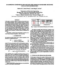
Figure 1: Single-diode equivalent circuit of a practical PV module.
been developed and demonstrated using PSCAD/EMTDC for parameter identification [29]. As this method is based on trial and error for different values of irradiance and temperature and is based on a large number of approximations and assumptions, this method becomes complicated and less accurate. Hence, to overcome the above drawbacks, an improved generalized method for evaluation of parameters, modeling, and simulation of photovoltaic modules has been proposed in this paper. A new concept “Level of Improvement” has been proposed for evaluating unknown parameters of the nonlinear I-V equation of the single-diode model of PV module including series and parallel resistances at any environmental condition (STC and NOCTC in this paper), taking the manufacturer-specified data at Standard Test Conditions as inputs. The new concept helps in improving the accuracy of the values of evaluated parameters up to various levels. The proposed evaluating method is based on mathematical equations of PV modules, thus making the method fast, simple, and accurate. The method for evaluating a is based on the property that at the maximum power point, dP/dV = 0. The proposed evaluating method is implemented by MATLAB programming and by using the values of parameters of the I-V equation obtained from programming results, a PV module model is build with MATLAB. The parameters evaluated by the proposed technique are validated with the datasheet values of six different commercially available PV modules for irradiance and temperature at Standard Test Conditions and Nominal Operating Cell Temperature Conditions. The module output characteristics generated by the proposed method are validated with experimental data of FS-270 PV module at different environmental conditions (varying irradiance and temperature). The effects of variation of ideality factor and resistances on the output characteristics are also studied. The superiority of the proposed technique over three popular existing techniques [4, 6, 12] is proved.
2. Mathematical Equation and Modeling of Photovoltaic Modules Practical modules are composed of various PV cells connected in series or parallel. Figure 1 shows the single-diode equivalent circuit of a practical PV module. The mathematical equation that describes the I-V characteristic of a practical PV module is
International Journal of Photoenergy I = I pv − I 0 exp
V + Rs I V + Rs I −1 − , V ta Rp
I = I pv,cell N p − I 0,cell N p exp
3
V + Rs I V + Rs I −1 − , V ta Rp
N s kT q
3.2. Evaluation of Diode Ideality Constant. By applying opencircuit condition (I = 0, V = V oc ) to (5), (8) can be derived as follows:
3
The equation that mathematically describes the P-V characteristic of a practical PV module is P = V I pv − I 0 exp
V + Rs I V + Rs I −1 − V ta Rp
K TV mpp , K TImpp , K TV oc , and K TIsc for any environmental condition. Table 1 shows the values of the parameters of seven different commercially available photovoltaic modules at STC provided by the manufacturers [30–36]. Some of the parameters of (4) can be found in the manufacturer’s datasheets. The remaining parameters such as I pv , a, I 0 , Rs , and Rp have to be evaluated. They are usually not specified by the manufacturers because they cannot be measured and are unique for every module [19].
3. Basic Evaluation of the Parameters The proposed work attempts to evaluate the five unknown parameters (I pv , a, I 0 , Rs , and Rp ) of a PV module at different environmental conditions. 3.1. Evaluation of Photovoltaic Current. The parallel resistance Rp is generally very high, so the last term of (1) can be eliminated for the further work. V + Rs I −1 V ta
5
By applying short-circuit condition (I = I sc , V = 0) to (5), (6) can be derived as follows: I sc = I pv − I 0 exp
I sc Rs −1 V ta
0 = I pv − I 0 exp
6
Since (I 0 exp I sc Rs /V t a − 1 ≈ 0), (6) can be written as
V oc −1 V ta
8
By rearranging (8), (9) is obtained as follows: I0 =
4
For the observation of the characteristics of the PV module, it is required to evaluate all the parameters of (1) [6]. Datasheets generally give information about the parameters, characteristics, and performances of PV modules with respect to the Standard Test Condition (STC), which is taken as 1000 W/m2 solar irradiance and 25°C module temperature [30–36]. Some datasheets also give information about PV modules at Nominal Operating Cell Temperature Condition (NOCTC), which is generally taken as 800 W/m2 irradiance and 20°C ambient temperature. The parameters basically present in all PV module datasheets at STC and sometimes at NOCTC are as follows: Pmpp , V mpp , I mpp , V oc , I sc , K TPmpp ,
I = I pv − I 0 exp
7
The photovoltaic current of a PV module is approximately equal to the short-circuit current at any environmental condition. 2
Vt =
I pv ≈ I sc
1
I pv exp V oc /V t a − 1
9
In the proposed method, the maximum power point is considered for evaluating “a” using the property dP/dV = 0 at the maximum power point. P = VI,
10
1 dP dI I ⋅ = + V dV dV V
11
By applying maximum power condition to (11), (12) is obtained as follows: dI dV
+ mpp
I mpp =0 V mpp
12
By differentiating (5) and applying maximum power condition, (13) can be obtained as follows: dI dV
= mpp
−I 0 /V t exp V mpp + I mpp Rs /V t a a + I 0 /V t Rs exp V mpp + I mpp Rs /V t a
13
By substituting (13) in (12), (14) can be obtained as follows: aI mpp + I mpp Rs − V mpp I 0 /V t exp V mpp + I mpp Rs /V t a =0 a + I 0 /V t Rs exp V mpp + I mpp Rs /V t a V mpp
14 For (14) to be valid, the numerator of (14) must be zero as the denominator is finite. V mpp + I mpp Rs I aI mpp + I mpp Rs − V mpp 0 exp =0 Vt V ta 15 By applying maximum power point condition to (5) and rearranging terms, (16) and (17) can be obtained as follows: exp
V mpp + I mpp Rs I pv − I mpp + I 0 = , V ta I0 Rs =
16
I pv − I mpp + I 0 V mpp V ta − ln I mpp I0 I mpp 17
4
International Journal of Photoenergy
Table 1: Parameters of seven different commercially available PV modules at STC (25°C and 1000 W/m2) provided by the manufacturers [30–36]. Parameter
Thin film Shell ST40 FS-270
Monocrystalline Shell SQ 150-PC HIT-N240SE10
KD140GX-LFBS
Multicrystalline KD260GX-LFB2
KU265-6MCA
PmppSTC W
40
70
150
240
140
260
265
V mppSTC V
16.6
65.5
34
43.7
17.7
31.0
31.0
I mppSTC A
2.41
1.07
4.4
5.51
7.91
8.39
8.55
V ocSTC V
23.3
88.0
43.4
52.4
22.1
38.3
38.3
I scSTC A
2.68
1.23
4.8
5.85
8.68
9.09
°
°
°
°
−0.6%/ C
−0.25%/ C
−0.52%/ C
−0.30%/ C
−0.46%/ C
−0.45%/ C
−0.45%/°C
K TV mpp
−100 mV/°C
−0.34%/°C
−167 mV/°C
−0.131 V/°C
−0.52%/°C
−0.48%/°C
−0.48%/°C
K TImpp
−2.50 mA/°C
0.023%/°C
−2.38 mA/°C
2.105 mA/°C
0.0066%/°C
0.02%/°C
0.02%/°C
K TV oc
−100 mV/°C
−0.25%/°C
−161 mV/°C
−0.131 V/°C
−0.36%/°C
−0.36%/°C
−0.36%/°C
K TIsc
0.35 mA/°C
0.04%/°C
1.4 mA/°C
1.76 mA/°C
0.060%/°C
0.06%/°C
0.06%/°C
Ns
36
116
72
72
36
60
60
Np
1
1
1
1
1
1
1
By combining (16) and (17), (18) can be obtained as follows: aI mpp + I pv − I mpp + I 0 I pv − I mpp + I 0 2V mpp a ln − =0 I0 Vt
18
°
at any environmental condition, a relation between Rs and Rp will be obtained, that is, 21
Pmpp cal = Pmpp , Pmpp cal = V mpp I mpp = V mpp I pv − I 0 exp
Substituting (7) and (9) in (18), (19) is obtained as follows: I sc exp V oc /V t a − 1 I sc − I mpp + I sc / exp V oc /V t a − 1 a ln I sc / exp V oc /V t a − 1
°
9.26
K TPmpp
−
V mpp + Rs I mpp −1 V ta
V mpp + Rs I mpp Rp
= Pmpp ,
22
aI mpp + I sc − I mpp +
−
2V mpp Vt
=0
Rp =
V mpp V mpp + I mpp Rs V mpp I pv − V mpp I 0 exp V mpp + I mpp Rs /V t a + V mpp I 0 − Pmpp
19 When the data specified in the manufacturer’s datasheets are used, the left hand side of (19) becomes a function of “a” and it is denoted by f a . I sc exp V oc /V t a − 1 I sc − I mpp + I sc / exp V oc /V t a − 1 a ln I sc / exp V oc /V t a − 1
f a = aI mpp + I sc − I mpp +
2V mpp − Vt
20 Thus, “a” is found by solving f a = 0 with the help of MATLAB programming. 3.3. Evaluation of Diode Reverse Saturation Current. By (9), the diode reverse saturation current at any environmental condition can be obtained. 3.4. Evaluation of Series and Parallel Resistances. Equating the maximum power calculated by the P-V model of (4) (Pmpp cal ) to the power at the MPP from the datasheet (Pmpp )
23 According to (23), for any value of Rs , there will be a value of Rp that satisfies (21). It is required to find an only pair of Rs and Rp for the desired environmental condition that satisfies the model accurately. 3.4.1. Proposed Algorithm. In this work, Rs and Rp in (23) are calculated through the following steps: (a) Eliminating the last term of (4), as the value of the parallel resistance is high, the power calculated by the P-V model excluding Rp , Pwithout RP is obtained as follows: Pwithout Rp = V I pv − I 0 exp
V + Rsmax′ I without Rp V ta
−1 24
(b) Iterations are performed on (24) where Rsmax′ is slowly incremented starting from Rsmax′ = 0, till the
International Journal of Photoenergy
5
maximum of power calculated by the P-V model excluding Rp (max Pwithout Rp ) becomes approximately equal to the power at the MPP from the datasheet (Pmpp ). (c) Putting Rs = Rsmax in (23), the value of Rp obtained is negative. Iterations are performed again on (23), where Rs is slowly decremented starting from Rs = Rsmax , until a positive value for Rp is obtained. Hence, the maximum value of parallel resistance Rpmax is obtained and the corresponding value of series resistance is the maximum value of series resistance, Rsmax . (d) Putting Rs = 0 in (23), the minimum value of parallel resistance Rpmin is obtained as follows: Rpmin =
V mpp I pv − I 0 exp V mpp /V t a + I 0 − Pmpp /V mpp
4. Improving the Model The accuracy of the values of evaluated parameters (I pv , a, I 0 , Rs , and Rp ) is improved up to various levels by using “Level of Improvement.” 4.1. First Level of Improvement 4.1.1. Evaluation of Photovoltaic Current. By applying shortcircuit condition (I = I sc , V = 0) to (5), (26) can be derived as follows: 26
Since (I 0 1 exp I sc Rs /V t a1 − 1 ≈ 0), (26) can be written as I pv 1 ≈ I sc 1 +
Rs Rp
I01 =
I pv 1 − V oc /Rp exp V oc /V t a1 − 1
27
By (27), the first level of improved value of photovoltaic current of a PV module (I pv 1) at any environmental condition can be obtained.
29
By applying the same procedure as is applied on (5) to find the diode ideality constant on (1), an improved and more accurate value of diode ideality constant can be obtained, as the values of both Rs and Rp are taken into account. The function f a1 , where a1 is the first level of improved value of diode ideality constant, becomes f a1 =
(e) Initialising Rs = Rsmax and Rp = Rpmax , iterations are performed again on (4) where Rs is slowly decremented and the corresponding value of Rp is obtained, till the maximum of power calculated by the P-V model (max P ) becomes approximately equal to the power at the MPP from the datasheet (Pmpp ), while Rp > Rpmin . Thus, Rs and Rp are obtained.
I sc Rs RI − 1 − s sc V t a1 Rp
By rearranging (28), (29) is obtained as follows:
25
The value of Rpmin obtained by the proposed method is more accurate as compared to other methods [4, 12].
I sc = I pv 1 − I 0 1 exp
4.1.2. Evaluation of Diode Ideality Constant. By applying open-circuit condition (I = 0, V = V oc ) to (5), (28) can be derived as follows: V oc V 28 − 1 − oc 0 = I pv 1 − I 0 1 exp V t a1 Rp
Rp I sc 1 + +
Rs Rp
− I mpp
I sc 1 + Rs /Rp − V oc /Rp exp V oc /V t a1 − 1
− V mpp + Rs I mpp
30
−V mpp + Rs I mpp
− V t a1 V mpp − Rp I mpp − Rs I mpp Thus, “a1” is found by solving f a1 = 0 with the help of MATLAB programming. 4.1.3. Evaluation of Diode Reverse Saturation Current. By (29), the first level of improved value of diode reverse saturation current (I 0 1) at any environmental condition can be obtained. 4.1.4. Evaluation of Series and Parallel Resistances. By applying the same procedure as is applied to evaluate Rs and Rp , a first level of improved values of series resistance (Rs 1) and parallel resistance (Rp 1) for the desired environmental condition can be found. 4.2. Second Level of Improvement. Again by putting Rs = Rs 1 and Rp = Rp 1 in (27) and (30), a second level of improved value of photovoltaic current (I pv 2) and diode ideality constant (a2) can be obtained. As a consequence, a second level of improved value of diode reverse saturation current (I 0 2), series resistance (Rs 2), and parallel resistance (Rp 2) can be obtained. The improvement can go up to ith level (I pv i, ai, I 0 i, Rs i, and Rp i ), till the errors between the values of parameters evaluated by the proposed method and the values of parameters provided in manufacturer’s datasheet become minimum. It should also be noted that the value of diode ideality constant should not vary much in any level of improvement. This is possible only when the value of parallel resistance is high. In the proposed method, initialising the series and parallel resistances by their corresponding maximum values in
6
International Journal of Photoenergy Input Pmpp , Vmpp , I mpp , Voc , I sc , Ns STC STC STC STC STC
Start
(from the manufacturer’s datasheet) Evaluate basic I pv , aSTC, I 0 , Rs , R p STC STC STC STC Level of improvement i = 1
Evaluate I pv i, aSTCi, I 0 i, Rs i, R p i STC STC STC STC
i=i+1
Evaluate Pmpp, Vmpp, I mpp, Voc, I sc, at STC
Input the values of parameters from manufacturer’s datasheet
Errors ≤ 1%
No
Yes Print I pv i, aSTCi, I 0 i, Rs i, R p i STC STC STC STC
Stop
Figure 2: Flowchart for evaluation of five unknown parameters (I pvSTC , aSTC , I 0STC , RsSTC , and RpSTC ) of a PV module at STC.
every level of improvement helps in getting higher value of parallel resistance and also reduces the required number of iterations. In this paper, only the first level of improvement has been applied.
5. Dependence of Parameters of the Characteristic Equation of the PV Module on Irradiance and Temperature The V oc , I sc , V mpp , I mpp , and Pmpp of the PV module depend on both solar irradiance and temperature and can be calculated using the following equations: V oc = 1 + K GV oc log
G GSTC
V ocSTC + K TV oc ΔT , 31
I sc =
G I + K TIsc ΔT , GSTC scSTC
V mpp = 1 + K GV mpp log
G GSTC
32
G I + K TImpp ΔT , GSTC mppSTC
G G 1 + K GPmpp log Pmpp = GSTC GSTC PmppSTC + K TPmpp ΔT ,
36
6. Evaluation of Parameters of the Characteristic Equation of the PV Module at STC Applying STC to the above procedure and using the manufacturer-specified data at Standard Test Condition, five unknown parameters (I pvSTC , aSTC , I 0STC , RsSTC , and RpSTC ) of a PV module at STC can be evaluated. The flowchart for evaluation of five unknown parameters (I pvSTC , aSTC , I 0STC , RsSTC , and RpSTC ) of a PV module at STC is presented in Figure 2. Table 2 shows the first level of improved values of the parameters of seven different commercially available PV modules for the proposed model and evaluated parameters of seven different commercially available PV modules for the Rs model [6], Rs and Rp model [4], and two-diode model [12] at STC.
V mppSTC + K TV mpp ΔT , 33
I mpp =
ΔT = T − T STC
34
35
7. Evaluation of Parameters of the Characteristic Equation of the PV Module at NOCTC Using the manufacturer-specified data at STC and NOCTC in (31), (33), and (35) irradiance coefficients of V oc , V mpp , and Pmpp of the PV module can be calculated. Five unknown parameters of a PV module at NOCTC can be evaluated using the following equations:
International Journal of Photoenergy
GNOCTC I scSTC + K TIsc ΔT GSTC
I pv NOCTC 1 ≈ f aNOCTC 1 =
GNOCTC /GSTC
− −
RsNOCTC , RpNOCTC 1+
I scSTC + K TIsc ΔT
RsNOCTC RpNOCTC
−
GNOCTC I mppSTC + K TImpp ΔT GSTC −
1 + RsNOCTC /RpNOCTC
1 + K GV oc log GNOCTC /GSTC
V ocSTC + K TV oc ΔT
exp
1 + K GV oc log GNOCTC /GSTC
1 + K GV mpp log
GNOCTC GSTC
V mppSTC + K TV mpp ΔT
+ RsNOCTC
GNOCTC I mppSTC + K TImpp ΔT GSTC
1 + K GV mpp log
GNOCTC GSTC
V mppSTC + K TV mpp ΔT
+ RsNOCTC
GNOCTC I mppSTC + K TImpp ΔT GSTC
− V tNOCTC aNOCTC 1 − RpNOCTC
1 + K GV mpp log GNOCTC /GSTC
GNOCTC I mppSTC + K TImpp ΔT GSTC
GNOCTC /GSTC
I 0NOCTC 1 =
1+
GNOCTC I scSTC + K TIsc ΔT GSTC
RpNOCTC +
7
I scSTC + K TIsc ΔT exp
V ocSTC + K TV oc ΔT
/RpNOCTC
/V tNOCTC aNOCTC 1 − 1
37
V mppSTC + K TV mpp ΔT GNOCTC I mppSTC + K TImpp ΔT GSTC
− RsNOCTC
1 + RsNOCTC /RpNOCTC
−
1 + K GV oc log GNOCTC /GSTC
,
1 + K GV oc log GNOCTC /GSTC
V ocSTC + K TV oc ΔT
V ocSTC + K TV oc ΔT
/RpNOCTC
/V tNOCTC aNOCTC 1 − 1
By using the above equations and by applying the same procedure as is applied to find RsSTC and RpSTC , RsNOCTC and RpNOCTC can be obtained.
RpNOCTC 1 =
x , y 1 + K GV mpp log
x= +
V mppSTC + K TV mpp ΔT
−
GNOCTC GSTC
1 + K GV mpp log
V mppSTC + K TV mpp ΔT
GNOCTC GSTC
exp exp
GNOCTC I scSTC + K TIsc ΔT GSTC
1 + RsNOCTC /RpNOCTC 1 + K GV oc
1 + K GV mpp log GNOCTC /GSTC
V mppSTC + K TV mpp ΔT
1+
RsNOCTC RpNOCTC
−
log GNOCTC /GSTC
V mppSTC + K TV mpp ΔT
1 + K GV oc log GNOCTC /GSTC V ocSTC
+ K TV oc ΔT
V ocSTC + K TV oc ΔT
/RpNOCTC
/V tNOCTC aNOCTC 1 − 1
+ GNOCTC /GSTC I mppSTC + K TImpp ΔT
RsNOCTC 1
V tNOCTC aNOCTC 1 1 + K GV mpp log GNOCTC /GSTC
V mppSTC + K TV mpp ΔT
GNOCTC /GSTC I scSTC + K TIsc ΔT exp −
GNOCTC GSTC
V mppSTC + K TV mpp ΔT
GNOCTC /GSTC I scSTC + K TIsc ΔT
+
1 + K GV mpp log
GNOCTC I mppSTC + K TImpp ΔT RsNOCTC 1 , GSTC 1 + K GV mpp log
Table 2: First level of improved values of the parameters of seven different commercially available PV modules for the proposed model and evaluated parameters of seven different commercially available PV modules for the Rs model, Rs and Rp model, and two-diode model at STC.
8 International Journal of Photoenergy
Proposed model
Model
1881.9879
RpNOCTC Ω 14942.890
2.40133
1.21772
RsNOCTC Ω 4073.0256
0.24346
2.4789 × 10⁻⁵
1.67257
2.86595 1.2555 × 10⁻⁴
3.863519999
−0.046283
−0.074512
0.046921
3790.1388
0.33097
4.6055 × 10⁻⁹
1.21016
4.706751999
−0.023365
0.012071
0.045882
Monocrystalline Shell SQ 150-PC HIT-N240SE10
0.991872000
1.75584
2.150160000
I pvNOCTC A
0.058966
1.5043 × 10⁻⁵
0.012262
K GPmpp
−0.022004
aNOCTC
−0.093363
0.096490
I 0NOCTC A
0.084956
K GV mpp
Thin film Shell ST40 FS-270
K GV oc
Parameter
469.1091
0.02807
5.6770 × 10⁻⁵
1.74535
7.027328000
0.030671
−0.039787
0.067477
KD140GX-LFBS
552.7469
0.15316
4.8923 × 10⁻⁶
1.50015
7.359264000
0.053982
0.019829
0.055781
Multicrystalline KD260GX-LFB2
644.3563
0.14925
4.6342 × 10⁻⁶
1.49252
7.496895999
0.044600
0.019829
0.055781
KU265-6MCA
Table 3: Evaluated irradiance coefficients of V oc , V mpp, and Pmpp of seven different commercially available PV modules and evaluated parameters of seven different commercially available PV modules at NOCTC (45°C and 1000 W/m2) for the proposed model.
International Journal of Photoenergy 9
10
International Journal of Photoenergy
G = 1000 W/m2 T = 25°C
1.2 1.2301 1.2301 Current (A)
0.8
1.2300 12.3 1.2299
0.01
1.2299
0.008
0.6 Current (A)
Current (A)
1
1.2298
0.4
0
0.005
0.01 0.015 Voltage (V)
0.02
0.006 0.004 0.002
0.2
0
0
0
10
20
30
40
a = 0.5 Rs = 16.129769999558533 ohm Rp = 522.71875677004743 ohm a = 1.0 Rs = 12.917819999680129 ohm Rp = 667.02661539703404 ohm a = 1.5 Rs = 10.24407999978135 ohm Rp = 892.78819916566204 ohm
87.5 87.6 87.7 87.8 87.9 88 Voltage (V)
50 Voltage (V)
60
88.1
70
80
90
a = 3.10212 Rs = 3.4667200000142437 ohm Rp = 295078.68087951292 ohm a = 3.5 Rs = 1.2372099999996378 ohm Rp = −16338145758.240559 ohm
a = 2.0 Rs = 7.8986499998701429 ohm Rp = 1314.0282246369643 ohm a = 2.5 Rs = 5.7858499999501287 ohm Rp = 2418.8793173864774 ohm a = 3.0 Rs = 3.8472600000167367 ohm Rp = 13792.332332059254 ohm (a) I-V characteristics
G = 1000 W/m2 T = 25°C
70 60
Power (W)
50 40 0.6 0.5 Power (W)
30 20
0.4 0.3 0.2 0.1
10
0 87.4
0
0
10
20
a = 0.5 Rs = 16.129769999558533 ohm Rp = 522.71875677004743 ohm a = 1.0 Rs = 12.917819999680129 ohm Rp = 667.02661539703404 ohm a = 1.5 Rs = 10.24407999978135 ohm Rp = 892.78819916566204 ohm
30
87.5
40
87.6
87.7 87.8 Voltage (V)
50 Voltage (V)
87.9
60
a = 2.0 Rs = 7.8986499998701429 ohm Rp = 1314.0282246369643 ohm a = 2.5 Rs = 5.7858499999501287 ohm Rp = 2418.8793173864774 ohm a = 3.0 Rs = 3.8472600000167367 ohm Rp = 13792.332332059254 ohm
88
70
88.1
80
90
a = 3.10212 Rs = 3.4667200000142437 ohm Rp = 295078.68087951292 ohm a = 3.5 Rs = 1.2372099999996378 ohm Rp = −16338145758.240559 ohm
(b) P-V characteristics
Figure 3: Characteristics for eight values of aSTC and the corresponding values of RsSTC and RpSTC of the FS-270 PV module at 25°C and 1000 W/m2.
a = 2.2104 Rs = 7.0000000000000000 ohm Rp = 1611.8581365886257 ohm a = 1.5506 Rs = 10.000000000000000 ohm Rp = 915.85035428054393 ohm
a = 3.10212 Rs = 3.4667200000142437 ohm Rp = 295078.68087951292 ohm a = 2.9618 Rs = 4.0000000000000000 ohm Rp = 10094.721742598975 ohm
88.1
80
90
a = 0.6630 Rs = 15.000000000000000 ohm Rp = 562.17132027512491 ohm a = 0.1817 Rs = 20.000000000000000 ohm Rp = -70421722.365352079 ohm
(a) I-V characteristics
80
G = 1000 W/m2 T = 25°C
70 60
0.6
40
0.5 Power (W)
Power (W)
50
30 20
0.4 0.3 0.2 0.1
10 0
0
0
10
20
20
a = 3.10212 Rs = 3.4667200000142437 ohm Rp = 295078.68087951292 ohm a = 2.9618 Rs = 4.0000000000000000 ohm Rp = 10094.721742598975 ohm
30
87.5
40
87.6
87.7
87.8 87.9 Voltage (V)
50 Voltage (V)
60
a = 2.2104 Rs = 7.0000000000000000 ohm Rp = 1611.8581365886257 ohm a = 1.5506 Rs = 10.000000000000000 ohm Rp = 915.85035428054393 ohm
88
88.1
70
88.2
80
90
a = 0.6630 Rs = 15.000000000000000 ohm Rp = 562.17132027512491 ohm a = 0.1817 Rs = 20.000000000000000 ohm Rp = -70421722.365352079 ohm
(b) P-V characteristics
Figure 4: Characteristics for six values of RsSTC and the corresponding values of aSTC and RpSTC of the FS-270 PV module at 25°C and 1000 W/m2.
12
International Journal of Photoenergy 1.8
T = 25°C
1.6 1.4
Current (A)
1.2 1 0.8 0.6 0.4 0.2 0
0
10
20
30
40
50
60
70
80
90
100
Voltage (V) G = 200 W/m2 a = 4.62046 Ipv = 0.24600 I0 = 1.11831 × 10‒3
G = 600 W/m2 a = 3.53568 Ipv = 0.73799 I0 = 2.63111 × 10‒4
G = 1000 W/m2 a = 3.10212 Ipv = 1.23000 I0 = 9.0404 × 10‒5
G = 400 W/m2 a = 3.89350 Ipv = 0.49199 I0 = 4.89851 × 10‒4
G = 800 W/m2 a = 3.29227 Ipv = 0.98399 I0 = 1.52035 × 10‒4
G = 1200 W/m2 a = 2.95556 Ipv = 1.47600 I0 = 5.67624 × 10‒5
(a) I-V characteristics
90 T = 25°C
80 70
Power (W)
60 50 40 30 20 10 0
0
10
20
30
40
50
60
70
80
90
100
Voltage (V) G = 200 W/m2 a = 4.62046 Ipv = 0.24600 I0 = 1.11831 × 10⁻³
G = 600 W/m2 a = 3.53568 Ipv = 0.73799 I0 = 2.63111 × 10⁻⁴
G = 1000 W/m2 a = 3.10212 Ipv = 1.23000 I0 = 9.0404 × 10⁻⁵
G = 400 W/m2 a = 3.89350 Ipv = 0.49199 I0 = 4.89851 × 10⁻⁴
G = 800 W/m2 a = 3.29227 Ipv = 0.98399 I0 = 1.52035 × 10⁻⁴
G = 1200 W/m2 a = 2.95556 Ipv = 1.47600 I0 = 5.67624 × 10⁻⁵
(b) P-V characteristics
Figure 5: Characteristics and experimental data of the FS-270 PV module at different irradiances (temperature constant = 25°C).
International Journal of Photoenergy
13
1.4 1.2 G = 1000 W/m2
Current (A)
1 0.8 0.6 0.4 0.2 0
0
10
20
30
40
50
60
70
80
90
100
Voltage (V) T = 0ºC a = 3.67198 Ipv = 1.21770 I0 = 1.08518 × 10⁻⁴
T = 45ºC a = 2.69645 Ipv = 1.23984 I0 = 7.23679 × 10⁻⁵
T = 25ºC a = 3.10212 Ipv = 1.23000 I0 = 9.0404 × 10⁻⁵
T = 60ºC a = 2.40938 Ipv = 1.24722 I0 = 5.61856 × 10⁻⁵
T = 75ºC a = 2.13729 Ipv = 1.25459 I0 = 4.00542 × 10⁻⁵
(a) I-V characteristics
80 70 G = 1000 W/m2
60
Power (W)
50 40 30 20 10 0
0
10
20
30
40
50
60
70
80
90
100
Voltage (V) T = 0ºC a = 3.67198 Ipv = 1.21770 I0 = 1.08518 × 10⁻⁴
T = 45ºC a = 2.69645 Ipv = 1.23984 I0 = 7.23679 × 10⁻⁵
T = 25ºC a = 3.10212 Ipv = 1.23000 I0 = 9.0404 × 10⁻⁵
T = 60ºC a = 2.40938 Ipv = 1.24722 I0 = 5.61856 × 10⁻⁵
T = 75ºC a = 2.13729 Ipv = 1.25459 I0 = 4.00542 × 10⁻⁵
(b) P-V characteristics
Figure 6: Characteristics and experimental data of the FS-270 PV module at different temperatures (irradiance constant = 1000 W/m2).
14
International Journal of Photoenergy 30
Relative error (%)
25
20
15
10
5
0
0
5
10
15
20 25 Voltage (V)
Curve 1 Curve 2
30
35
40
45
Curve 3 Curve 4
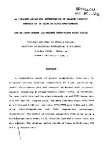
Figure 7: Relative errors of the model proposed in this paper (curve 1), in [4] (curve 2), in [12] (curve 3), and in [6] (curve 4) for the FS-270 PV module at 25°C and 1000 W/m2. Table 4: Comparison of Rs model, Rs and Rp model, two-diode model, and proposed model output with manufacturer’s datasheet for Shell ST40 PV module [30]. Environmental Datasheet Parameter conditions value
STC (25°C and 1000 W/m2)
NOCTC (47°C and 800 W/m2)
Rs Rs and Rp Two-diode model model value model value value
Proposed model value
Error Rs (%)
Error Rs and Rp (%) −0.0012
0.0150
Error Error twoproposed diode (%) (%)
Pmpp W
40
29.0224
40.0055
40.0060
40.0000
−27.4589
V mpp V
16.6
14.9120
16.7760
16.6000
16.6029
−10.1686
1.0602
0.0000
0.0174
I mpp A
2.41
1.9462
2.3847
2.4100
2.4098
−19.2448
−1.0497
0.0000
−0.0082
V oc V I sc A
23.3 2.68
21.0254 2.1590
23.2618 2.6646
23.2460 2.6578
23.2993 2.6800
−9.7622 −19.4402
−0.1639 −0.5746
−0.2317 −0.8283
−0.0030 0.0000
0.0000
Pmpp W
27.7
19.5088
28.2982
28.5162
27.7024
−29.5711
2.1595
2.9465
0.0086
V mpp V
14.7
12.6790
14.9120
14.9120
14.6933
−13.7482
1.4421
1.4421
−0.0455
V oc V I sc A
20.7 2.2
18.8271 1.7502
20.7820 2.1378
20.8002 2.1324
20.7009 2.1982
−9.0478 −20.4454
0.3961 −2.8272
0.4840 −3.0727
0.0043 −0.0818
Table 5: Comparison of Rs model, Rs and Rp model, two-diode model, and proposed model output with manufacturer’s datasheet for Shell SQ 150-PC PV module [32]. Rs model value
Rs and Rp model value
Two-diode model value
Proposed model value
Error Rs (%)
Error Rs and Rp (%)
150
111.6218
149.5998
149.6000
150.0000
−25.5854
−0.2668
V mpp V
34
30.3800
34.2860
34.0000
34.0115
−10.6470
0.8411
0.0000
0.0338
I mpp A
4.4
3.6742
4.3633
4.4000
4.3998
−16.4954
−0.8340
0.0000
−0.0045
V oc V I sc A
43.4 4.8
39.7399 3.9475
43.3302 4.7848
43.3012 4.7843
43.3972 4.8000
−8.4334 −17.7604
−0.1608 −0.3166
−0.2276 −0.3270
−0.0064 0.0000
Pmpp W
108
85.7801
107.7001
107.8484
107.9950
−20.5739
−0.2776
−0.1403
−0.0046
V mpp V
31
26.3800
30.8140
30.8140
30.9800
−14.9032
−0.5999
−0.5999
−0.0645
V oc V I sc A
39.6 3.9
36.4498 3.3635
39.4670 3.8513
39.4310 3.8509
39.5964 3.8985
−7.9550 −13.7564
−0.3358 −1.2487
−0.4267 −1.2589
−0.0090 −0.0384
Environmental Datasheet Parameter conditions value Pmpp W STC (25°C and 1000 W/m2)
NOCTC (46°C and 800 W/m2)
Error Error twoproposed diode (%) (%) −0.2666
0.0000
International Journal of Photoenergy
15
Table 6: Comparison of Rs model, Rs and Rp model, two-diode model, and proposed model output with manufacturer’s datasheet for HIT-N240SE10 PV module [33]. Datasheet Environmental Parameter value conditions
STC (25°C and 1000 W/m2)
NOCTC (44°C and 800 W/m2)
Rs model value
Rs and Rp Two-diode model value model value
Proposed model value
Error Rs (%)
Error Rs and Rp (%)
Error Error twoproposed diode (%) (%)
Pmpp W
240
186.2506
240.7864
240.7870
240.0000
−22.3955
0.3276
0.3279
0.0000
V mpp V
43.7
40.8720
44.0160
43.7000
43.7008
−6.4713
0.7231
0.0000
0.0018
I mpp A
5.51
4.5569
5.4704
5.5100
5.5096
−17.2976
−0.7186
0.0000
−0.0072
V oc V I sc A
52.4 5.85
49.3547 4.8447
52.3588 5.8443
52.3470 5.8436
52.3988 5.8500
−5.8116 −17.1846
−0.0786 −0.0974
−0.1011 −0.1094
−0.0022 0.0000
Pmpp W
182
149.8145
180.5653
180.9046
181.9713
−17.6843
−0.7882
−0.6018
−0.0157
V mpp V
41.1
37.8720
41.3960
41.3960
41.0970
−7.8540
0.7201
0.7201
−0.0072
I mpp A
4.44
3.6484
4.3619
4.3701
4.4396
−17.8288
−1.7590
−1.5743
−0.0090
V oc V I sc A
49.4 4.71
45.5426 3.8068
49.3914 4.7021
49.3938 4.7016
49.3992 4.7098
−7.8085 −19.1762
−0.0174 −0.1677
−0.0125 −0.1783
−0.0016 −0.0042
Table 7: Comparison of Rs model, Rs and Rp model, two-diode model, and proposed model output with manufacturer’s datasheet for KD140GX-LFBS PV module [34]. Datasheet Environmental Parameter value conditions
STC (25°C and 1000 W/m2)
NOCTC (45°C and 800 W/m2)
Rs model value
Rs and Rp Two-diode model value model value
Proposed model value
Error Rs (%)
Error Rs and Rp (%)
Error Error twoproposed diode (%) (%)
Pmpp W
140
112.2240
139.9971
140.0070
140.0000
−19.8399
−0.0020
0.0050
0.0000
V mpp V
17.7
15.9120
17.9010
17.7000
17.7007
−10.1016
1.1355
0.0000
0.0039
I mpp A
7.91
7.0528
7.8206
7.9100
7.9091
−10.8369
−1.1302
0.0000
−0.0113
V oc V I sc A
22.1 8.68
20.3590 7.6673
22.0514 8.6514
22.0396 8.6491
22.1000 8.6800
−7.8778 −11.6670
−0.2199 −0.3294
−0.2733 −0.3559
0.0000 0.0000
Pmpp W
101
79.3291
101.7994
101.9756
100.9936
−21.4563
0.7914
0.9659
−0.0063
V mpp V
16.0
14.6910
16.1330
16.1330
15.9880
−8.1812
0.8312
0.8312
−0.0750
I mpp A
6.33
5.5852
6.3100
6.3209
6.3278
−11.7661
−0.3159
−0.1437
−0.0347
V oc V I sc A
20.2 7.03
18.0738 6.4273
20.2155 7.0042
20.2034 7.0023
20.1983 7.0293
−10.5257 −8.5732
0.0767 −0.3669
0.0168 −0.3940
−0.0084 −0.0099
Table 8: Comparison of Rs model, Rs and Rp model, two-diode model, and proposed model output with manufacturer’s datasheet for KD260GX-LFB2 PV module [35]. Environmental Datasheet Parameter conditions value
STC (25°C and 1000 W/m2)
NOCTC (45°C and 800 W/m2)
Rs model value
Rs and Rp Two-diode model value model value
Proposed model value
Error Rs (%)
Error Rs and Rp (%)
Error Error twoproposed diode (%) (%)
Pmpp W
260
208.7319
260.0899
260.0900
260.0000
−19.7185
0.0345
0.0346
0.0000
V mpp V
31.0
27.5760
31.0230
31.0000
31.0022
−11.0451
0.0741
0.0000
0.0070
I mpp A
8.39
7.5693
8.3838
8.3900
8.3895
−9.7818
−0.0738
0.0000
−0.0059
V oc V I sc A
38.3 9.09
35.2913 8.0652
38.2471 9.0739
38.2249 9.0685
38.2994 9.0900
−7.8556 −11.2739
−0.1381 −0.1771
−0.1960 −0.2365
−0.0015 0.0000
Pmpp W
187
142.6852
189.3933
189.8687
186.9801
−23.6977
1.2798
1.5340
−0.0106
V mpp V
27.9
24.7590
28.3420
28.3420
27.8997
−11.2580
1.5842
1.5842
−0.0010
I mpp A
6.71
5.8309
6.6824
6.6992
6.7096
−13.1013
−0.4113
−0.1609
−0.0059
V oc V I sc A
35.1 7.36
33.8348 6.1593
35.0769 7.3462
35.0657 7.3418
35.0982 7.3597
−3.6045 −16.3138
−0.0658 −0.1875
−0.0977 −0.2472
−0.0051 −0.0040
16
International Journal of Photoenergy
Table 9: Comparison of Rs model, Rs and Rp model, two-diode model, and proposed model output with manufacturer’s datasheet for KU265-6MCA PV module [36]. Environmental Datasheet Parameter conditions value
STC (25°C and 1000 W/m2)
NOCTC (45°C and 800 W/m2)
Rs model value
Rs and Rp model value
Two-diode model value
Proposed model value
Error Rs (%)
Error Rs and Rp (%) 0.0188
Error Error twoproposed diode (%) (%)
Pmpp W
265
213.0696
265.0499
265.0500
265.0000
−19.5963
V mpp V
31.0
27.5760
31.0230
31.0000
31.0030
−11.0451
0.0741
0.0000
0.0096
I mpp A
8.55
7.7266
8.5437
8.5500
8.5490
−9.6304
−0.0736
0.0000
−0.0116
V oc V I sc A
38.3 9.26
35.2946 8.2312
38.2529 9.2439
38.2234 9.2378
38.3000 9.2600
−7.8469 −11.1101
−0.1229 −0.1738
−0.1999 −0.2397
0.0000 0.0000
Pmpp W
191
147.6087
193.0154
193.4476
190.9769
−22.7179
1.0551
1.2814
−0.0120
V mpp V
27.9
24.5590
28.3420
28.3420
27.8975
−11.9749
1.5842
1.5842
−0.0089
I mpp A
6.85
5.5069
6.8102
6.8255
6.8496
−19.6072
−0.5810
−0.3576
−0.0058
V oc V I sc A
35.1 7.49
33.6348 6.9605
35.0778 7.4838
35.0639 7.4789
35.0975 7.4902
−4.1743 −7.0694
−0.0632 −0.0827
−0.1028 −0.1481
−0.0071 0.0026
0.0188
0.0000
Rs -K-
1 G 2 Ki 3 T
×
+ ‒
×
++
25 4 I (sc,STC)
× ÷
1 Ipv
× ÷
9 Rp
++
10 V
×
×
1000 G (STC)
T (STC) C
× ÷
++
× ÷
3 I0
eu
+ ‒
×
+ ‒ ‒ 5
++ 5 Ns
× ÷
eu
+ ‒
I
1
×
× 1
-Ck
×
6 a
÷ ×
eu
+ ‒
× ÷
+ ‒ 2 I (0,STC)
1
8 Kv
×
× ×
×
298
× ÷
++
T (STC )K 7 V (oc,STC)
4 P
×
273
-Cq
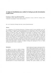
Figure 8: Detailed implementation of PV module model in MATLAB/Simulink that solves the I-V equation.
Table 3 shows the evaluated irradiance coefficients of V oc , V mpp , and Pmpp of seven different commercially available PV modules and evaluated parameters of seven different commercially available PV modules at NOCTC for the proposed model. It is evident from the above equations that all the parameters of the characteristic equation of the PV module are subject to vary with irradiance and temperature, which is a truism. This increases the accuracy of the proposed method of evaluating parameters manifold as compared to existing methods in this area where the parameters are assumed constant [4, 6, 12]. The proposed model output characteristics very accurately match the experimental
output characteristics and manufacturer’s datasheets which is authenticated from the results shown in the later sections.
8. Curves and Inferences As shown in Figures 3(a) and 3(b), I-V and P-V curves of the FS-270 PV module are generated for eight values of aSTC and the corresponding values of RsSTC and RpSTC . It can be noted that as the value of aSTC calculated by the proposed method is utilised, the value of V ocSTC obtained from the proposed model becomes closest to the datasheet value. I-V and P-V curves of the FS-270 PV module are plotted again for six values of RsSTC and the corresponding values of aSTC and
International Journal of Photoenergy
1
17
R
s
G
G 2
-KK
Ki 3
i Ipv
T
1 a
Ipv
T 4
Tables 4–9 show the comparison of Rs model, Rs and Rp model, two-diode model, and proposed model output with manufacturer’s datasheets for six different commercially available PV modules [30–36]. In the proposed method, it has been assumed that all the PV cells of a module are perfectly made but this is not the case in reality. Still the proposed method confirms to be very accurate as can be clearly seen from Figure 7 and Tables 4–9. This is because the properties of the PV cells having the same parameters, manufactured from the same producer, do not vary much and hence can be assumed identical.
V (oc,STC)
I (sc,STC)
I (sc,STC)
9 Rp 10
Rp
V
V P
Photovoltaic current (Ipv)
8 Kv
I (sc,STC)
I (sc,STC)
IRs
Kv
3 I0
Ipv 5
5 Ns 6
Ki
Ns I (0,STC) a
2 I (0,STC)
V (oc,STC)
10. Simulation of the PV Module
T I
0
a 7 V (oc,STC)
P
T
I
Ns Diode reverse saturation current (I ) 0
a
4 I
Diode reverse saturation current (STC) (I (0,STC)) Ns Current (I), power (P)
Figure 9: PV module model with subsystems in MATLAB/ Simulink that solves the I-V equation.
RpSTC (see Figures 4(a) and 4(b)). As the value of RsSTC calculated by the proposed method is utilised, the value of V ocSTC obtained from the proposed model becomes closest to the datasheet value. Similar is the case with RpSTC . The accuracy of the model is highest, when the values of aSTC , RsSTC , and RpSTC calculated by the proposed technique are utilised for modeling. The proposed method of evaluating the unknown parameters is far more accurate as compared to other methods mentioned in literature.
9. Validation of the Model The current and power output obtained from the proposed model is validated against measured current and power output data, respectively, for the FS-270 PV module provided by the National Institute of Technology Patna (NITP), India. Figures 5(a) and 5(b) show the mathematical I-V and P-V characteristics of the FS-270 PV module [31] plotted with the experimental data by varying irradiance from 200 W/m2 to 1200 W/m2 at 25°C. Figures 6(a) and 6(b) show the I-V and P-V curves by varying temperature from 0°C to 75°C at 1000 W/m2. The experimental points are represented by circular markers in the curves. As the model is not perfect, some points are not exactly matched, although it is sufficiently accurate for majority points. The relative errors of the proposed model with respect to the experimental data for the FS-270 PV module at 25°C and 1000 W/m2 are shown in Figure 7. The model proposed in this paper is compared with the models proposed in [4, 6, 12]. The relative errors obtained by all the models are plotted on the same graphs. The model proposed in this paper is superior, because the values of relative errors obtained by the proposed model are very small as compared to other models.
The PV module model can be simulated in any circuit simulator by implementing (1) and (4) using basic math blocks. Figures 8 and 9 show a PV module model, where these two equations are implemented in MATLAB/Simulink. In the complete model, irradiance and temperature along with the evaluated and manufacturer-specified parameters of the PV module are the inputs while the outputs are current and power. The proposed model is most generalized as compared to the models proposed in previous works.
11. Conclusion In this paper, an improved generalized method for evaluation of parameters, modeling, and simulation of photovoltaic modules is proposed. The proposed PV module modeling method surpasses the other methods already published, as it has the following novelties: (i) A new concept “Level of Improvement” has been proposed for evaluating unknown parameters of the nonlinear I-V equation of the single-diode model of PV module at any environmental condition (STC and NOCTC in this paper), taking the manufacturer-specified data at Standard Test Conditions as inputs. (ii) The new method of evaluation of unknown parameters is based on mathematical equations of PV modules. By implementing simple set of equations using any software, the parameters can be determined numerically simply by feeding few manufacturerspecified data as input to the program. (iii) In this paper, for the first time, the effects of varying ideality factor and resistances on the output curves have been observed. It has been inferred that as the values of aSTC , RsSTC , and RpSTC calculated by the proposed method are utilised, the value of V ocSTC obtained from the proposed model becomes closest to the datasheet value. The accuracy of the model is maximum, when the values of aSTC , RsSTC , and RpSTC calculated by the proposed technique are utilised for modeling.
18
International Journal of Photoenergy (iv) A most generalized PV module model is build with MATLAB/Simulink by using the values of parameters of the I-V equation obtained from programming results in order to show the practical use of the proposed model. (v) The proposed method proves to be more accurate in modeling commercially available PV modules as compared to other methods available in literature.
K TIsc :
Temperature coefficient of I sc (A/K).
Index STC:
Subscripts indicate the parameters at Standard Test Condition NOCTC: Subscripts indicate the parameters at Nominal Operating Cell Temperature Condition.
12. Future Work
Conflicts of Interest
Under partial shading condition (PSC) on a PV array, the irradiance and temperature of the PV modules undergoing shading change. The parameters of the shaded and unshaded PV modules of the array can be easily evaluated by employing the proposed method. By applying a suitable maximum power point tracking (MPPT) technique, maximum power point (MPP) of a PV array under PSC can be reached and hence MPPT can be ensured which will be the subject of our further investigations.
The authors declare that there is no conflict of interest regarding the publication of this paper.
Nomenclature I pv,cell : Photovoltaic current of the ideal PV cell (A) I 0,cell : Reverse saturation or leakage current of the ideal PV cell (A) I pv : Photovoltaic current of the PV module (A) Reverse saturation or leakage current of the PV I0: module (A) a: Diode ideality constant of the PV module Rs : Equivalent series resistance of the PV module (Ω) Rp : Equivalent parallel resistance of the PV module (Ω) Thermal voltage of the PV module (V) V t: q: Electron charge (1 60217646 ∗ 10−19 C) k: Boltzmann constant (1 3806503 ∗ 10−23 J/K) G: Irradiance (W/m2) T: Temperature of the PV module (K) N s: Number of cells connected in series in the PV module N p: Number of parallel connections of cells in the PV module Pmpp : Power of the PV module at the maximum power point (W) V mpp : Voltage of the PV module at the maximum power point (V) I mpp : Current of the PV module at the maximum power point (A) V oc : Open-circuit voltage of the PV module (V) Short-circuit current of the PV module (A) I sc : K GPmpp : Irradiance coefficient of Pmpp K TP : Temperature coefficient of Pmpp (W/K) mpp
K GV mpp : Irradiance coefficient of V mpp K TV : Temperature coefficient of V mpp (V/K) mpp
K TImpp :
Temperature coefficient of I mpp (A/K)
K GV oc : K TV oc :
Irradiance coefficient of V oc Temperature coefficient of V oc (V/K)
Acknowledgments The authors wish to thank the Electrical Engineering Department of the National Institute of Technology Patna (India) for providing all the experimental facilities to carry out this work.
References [1] S. A. Rahman, R. Varma, and T. Vanderheide, “Generalised model of a photovoltaic panel,” IET Renewable Power Generation, vol. 8, no. 3, pp. 217–229, 2014. [2] P. H. Huang, W. Xiao, J. C. H. Peng, and J. L. Kirtley, “Comprehensive parameterization of solar cell: improved accuracy with simulation efficiency,” IEEE Transactions on Industrial Electronics, vol. 63, pp. 1549–1560, 2016. [3] X. Feng, X. Qing, C. Y. Chung, H. Qiao, X. Wang, and X. Zhao, “A simple parameter estimation approach to modeling of photovoltaic modules based on datasheet values,” Journal of Solar Energy Engineering, vol. 138, no. 5, article 0510108, 2016. [4] M. G. Villalva, J. R. Gazoli, and E. R. Filho, “Comprehensive approach to modeling and simulation of photovoltaic arrays,” IEEE Transactions on Power Electronics, vol. 24, no. 5, pp. 1198–1208, 2009. [5] W. De Soto, S. A. Klein, and W. A. Beckman, “Improvement and validation of a model for photovoltaic array performance,” Solar Energy, vol. 80, no. 1, pp. 78–88, 2006. [6] G. R. Walker, “Evaluating MPPT converter topologies using a MATLAB PV model,” Journal of Electrical and Electronics Engineering, vol. 21, no. 1, pp. 49–55, 2001. [7] H. N. Mohamed and S. A. Mahmoud, “Temperature dependence in modeling photovoltaic arrays,” in 2013 IEEE 20th International Conference on Electronics, Circuits, and Systems (ICECS), pp. 747–750, Abu Dhabi, United Arab Emirates, 2013. [8] V. J. Chin, Z. Salam, and K. Ishaque, “An accurate modelling of the two-diode model of PV module using a hybrid solution based on differential evolution,” Energy Conversion and Management, vol. 124, p. 4250, 2016. [9] B. C. Babu and S. Gurjar, “A novel simplified two-diode model of photovoltaic (PV) module,” IEEE Journal of Photovoltaics, vol. 4, pp. 1156–1161, 2014. [10] D. H. Muhsen, A. B. Ghazali, T. Khatib, and I. A. Abed, “Parameters extraction of double diode photovoltaic module’s model based on hybrid evolutionary algorithm,” Energy Conversion and Management, vol. 105, pp. 552–561, 2015.
International Journal of Photoenergy [11] J. A. Gow and C. D. Manning, “Development of a photovoltaic array model for use in power-electronics simulation studies,” IEE Proceedings - Electric Power Applications, vol. 146, no. 2, pp. 193–200, 1999. [12] K. Ishaque, Z. Salam, and H. Taheri, “Simple, fast and accurate two-diode model for photovoltaic modules,” Solar Energy Materials and Solar Cells, vol. 95, no. 2, pp. 586–594, 2011. [13] S. Lun, S. Wang, T. Guo, and C. Du, “An I–V model based on time warp invariant echo state network for photovoltaic array with shaded solar cells,” Solar Energy, vol. 105, pp. 529–541, 2014. [14] A. Oi, Design and simulation of photovoltaic water pumping system, [M.S. thesis], Faculty of California Polytechnic State University, San Luis Obispo, CA, USA, 2005. [15] MATLAB demos, “Solar cell parameter extraction from data,” November 2017, http://in.mathworks.com/help/physmod/elec /examples/solar-cell-parameter-extraction-from-data.html. [16] “Solar panels, 5th Generation a-Si solar panels, Datasheet,” November 2017, http://www.apexpowerconcepts.com/fee-2012.pdf. [17] A. N. Celik and N. Acikgoz, “Modelling and experimental verification of the operating current of mono-crystalline photovoltaic modules using four- and five-parameter models,” Applied Energy, vol. 84, no. 1, pp. 1–15, 2007. [18] I. H. Altas and A. M. Sharaf, “A photovoltaic array simulation model for Matlab-Simulink GUI environment,” in 2007 International Conference on Clean Electrical Power, pp. 341–345, Capri, Itlay, 2007. [19] N. N. B. Ulapane, C. H. Dhanapala, S. M. Wickramasinghe, S. G. Abeyratne, N. Rathnayake, and P. J. Binduhewa, “Extraction of parameters for simulating photovoltaic panels,” in 2011 6th International Conference on Industrial and Information Systems, Kandy, Sri Lanka, August 2011. [20] M. C. Glass, “Improved solar array power point model with SPICE realization,” in IECEC 96. Proceedings of the 31st Intersociety Energy Conversion Engineering Conference, pp. 286– 291, Washington, DC, USA, August 1996. [21] Y. T. Tan, D. S. Kirschen, and N. Jenkins, “A model of PV generation suitable for stability analysis,” IEEE Transactions on Energy Conversion, vol. 19, no. 4, pp. 748–755, 2004. [22] T. Aernouts, W. Geens, J. Poortmans, P. Heremans, S. Borghs, and R. Mertens, “Extraction of bulk and contact components of the series resistance in organic bulk donor-acceptor-heterojunctions,” Thin Solid Films, vol. 403-404, pp. 297–301, 2002. [23] D. S. H. Chan and J. C. H. Phang, “Analytical methods for the extraction of solar-cell single- and double-diode model parameters from I-V characteristics,” IEEE Transactions on Electron Devices, vol. 34, no. 2, pp. 286–293, 1987. [24] S.-x. Lun, S. Wang, G.-h. Yang, and T.-t. Guo, “A new explicit double-diode modeling method based on Lambert W-function for photovoltaic arrays,” Solar Energy, vol. 116, pp. 69–82, 2015. [25] T. F. Elshatter, M. T. Elhagree, M. E. Aboueldahab, and A. A. Elkousry, “Fuzzy modeling and simulation of photovoltaic system,” in Proceedings of the 14th European Photovoltaic Solar Energy Conference, 1997. [26] A. Mellit, M. Benghanem, and S. A. Kalogirou, “Modeling and simulation of a stand-alone photovoltaic system using an adaptive artificial neural network: proposition for a new sizing procedure,” Renewable Energy, vol. 32, pp. 285–313, 2007.
19 [27] F. Almonacid, C. Rus, L. Hontoria, and F. J. Munoz, “Characterisation of PV CIS module by artificial neural networks. A comparative study with other methods,” Renewable Energy, vol. 35, pp. 973–980, 2010. [28] S. Jing Jun and L. Kay-Soon, “Photovoltaic model identification using particle swarm optimization with inverse barrier constraint,” IEEE Transactions on Power Electronics, vol. 27, no. 9, pp. 3975–3983, 2012. [29] R. C. Campbell, “A circuit-based photovoltaic array model for power system studies,” July 2010, http://www.ee.washington. edu/research/sesame/publication/Conference/2007/Campbell_ PWL_PV_Model_NAPS2007.pdf. [30] “Shell solar product information sheet,” http://www.atlanta solar.com/pdf/Shell/ShellST40_USv1.pdf. [31] “First solar FS-270 (70W) solar panel,” September 2017, http:// www.firstsolar.com/en-IN/-/media/First-Solar/TechnicalDocuments/Series-2-Datasheets/Series-2-Module-DatasheetNA.ashx?la=en. [32] “Shell solar product information sheet,” http://www.physics. arizona.edu/~cronin/Solar/TEP%20module%20spec%20sheets/ Shell%20SQ150.pdf. [33] “HIT photovoltaic module, HIT-N240SE10 HIT-N235SE10 HIT N230SE10 datasheet,” 2017, http://future-energy-solutions. co.uk/wp-content/uploads/2014/10/Panasonic-Datasheet-HIT240W.pdf. [34] “KD140GX-LFBS, KD 135 F series - Kyocera Solar datasheet,” http://www.kyocerasolar.com/dealers/product-center/. [35] “KD260GX-LFB2, KD 200-60F series - Kyocera Solar datasheet,” http://www.kyocerasolar.com/dealers/product-center/. [36] “KU265-6MCA, KU 200-60F series - Kyocera Solar atasheet,” http://www.kyocerasolar.com/dealers/product-center/.