An Improved Interest Point Matching Algorithm for ...

IEEE IPAS’14: INTERNATIONAL IMAGE PROCESSING APPLICATIONS AND SYSTEMS CONFERENCE 2014

1

An Improved Interest Point Matching Algorithm for Human Body Tracking Alireza Dehghani∗ , Alistair Sutherland∗ , David Moloney† and Dexmont Pe˜na∗ ∗ School of Computing, Dublin City University, Dublin, Ireland. Emails: [email protected], [email protected], [email protected] † Movidius Ltd., Dublin, Ireland. Email: [email protected]

Abstract—The interest point (IP) matching algorithms match the points either locally or spatially. We propose a local-spatial IP matching algorithm usable for articulated human body tracking. The local-based stage finds matched IP pairs of two reference and target IP lists using a local-feature-descriptors-based matching method. Then, the spatial-based stage recovers more matched pairs from the remaining unmatched IPs through based on the result of the previous stage using the Shape Contexts (SC) feature vectors. The proposed approach benefits from the speed of local matching algorithms as well as the accuracy and robustness of spatial matching methods. Experimental results show that not only the proposed algorithm increases the precision rate from 44.71% to 97.41%, but also it improves the recall rate from 80.88% to 84.96%. Index Terms—Interest Points Matching, Shape Contexts, Human Body Tracking.

I. I NTRODUCTION The Interest Point (IP) matching is a crucial and challenging process, which is widely used in several IP-based Computer Vision (CV) applications such as image registration, object detection and classification, and object and human motion tracking. It aims to find a reliable correspondence between two sets of IPs, which are called the Ref-set and Tar-set from now on in this paper, using some local and/or spatial similarity criteria. The local-based IP matching methods mainly use local feature descriptors to measure local similarity among the points, while the spatial-based ones use geometric distance and spatial structure [1]. Local feature descriptors have been studied widely [2]. They use different properties of image such as pixel intensities, colour, texture, and edges to describe the local property of a neighbourhood around any specific location of image. These information are used to measure the similarity between IPs in local-based IP matching algorithms. Many remarkable local feature descriptors such as the Scale Invariant Feature Transform (SIFT) [3], Speeded Up Robust Features (SURF) [4], and Gradient Location and Orientation Histogram (GLOH) [2] have been proposed in the literature. The ORB (Oriented FAST and Rotated BRIEF) [5], which is rotation-invariant and resistant to noise, performs same as SIFT and better than SURF, while being twice as fast. These local descriptors have achieved an appreciable level of matureness to use in IP matching applications [6]. However, they may collapse in some ambiguous situations such as 978-1-4799-7069-8/14/$31.00 2014 IEEE

monotonous backgrounds, similar features, low resolution images. Consequently, several mismatched pairs could be found in the result. In these cases, the spatial-based IP matching methods, which use information like geometric distance or neighbourhood relations among points, can be used to compensate for these drawbacks. Similar to local-based IP matching algorithms, noteworthy methods have been also proposed by many authors. The iterative RANdom SAmple Consensus (RANSAC) [7], which fits a mathematical model to a set of points including outliers, can be reasonably used only when there are reasonable level of outliers. Iterative Closest Point (ICP) [8] is another simple and straightforward method, which works well only under a good initial estimation. Consideration of local relations between IPs [9], graph establishment by Delaunay triangulation in a twostep algorithm [10], a Graph Transformation Matching (GTM) strategy for finding a consensus nearest neighbour graph from candidate matches [11], and using relative positions and angles of points for reduction of false matching are some example of methods which the spatial relation between points has been dealt with. Although the spatial-based methods are more accurate and robust than the local-based ones, they are not as quick, particularly when there is a high number of IPs. It is because, these approaches compare the IPs of Ref-set and Tar-set mutually in an iterative way to find the best matched pairs [9]. This makes them computationally expensive. Since the tracking applications deal with smooth and small inter-frame motions usually [12], these extra iterative calculations can be kept away. To do this, a fast and efficient local-based matching method followed by a supplementary spatial-based procedure, which form together a combined approaches [13], is proposed to complement each other. In this way, the local-based IP matching approach cuts down efficiently the search space that the spatial-based method needs, whilst the spatial-based approach compensate for the defects of local-based methods in ambiguous situations. In summary, we propose an improved IP matching algorithm in this paper which can be used in tracking as well as the other CV applications. Firstly, the confidently matched pairs are found using a local-based IP matching strategy followed by two filtering process. Then, a spatial-based matching procedure based on Shape Context (SC) is used to compensate for the filtered out mismatched pairs as well as the remaining unmatched IPs. The proposed approach benefits from: local-

IEEE IPAS’14: INTERNATIONAL IMAGE PROCESSING APPLICATIONS AND SYSTEMS CONFERENCE 2014

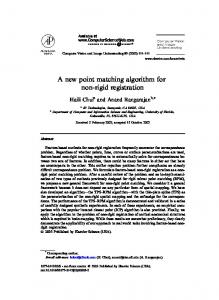
based IP matching to avoid the expense of the distance and neighbourhood comparison of the spatial-based methods; spatial-based IP matching to compensate for the drawback of the local-based methods. The rest of this paper is outlined as follow: Section II presents the proposed algorithm. Experimental results and conclusions will be discussed in Sections III and IV, respectively. II. I NTEREST P OINT M ATCHING A LGORITHM To increase the readability of paper, the local and spatial matching procedures of our proposed algorithm are discussed separately in Sections II-A, II-B, respectively. A. Local-Based IP Matching Firstly, the extracted IPs of reference and target images are stored into the Ref-set and Tar-set, respectively. To perform the local-based IP matching, the local feature descriptors of IPs of two sets are extracted. Using these descriptors, IPs of two sets are matched to each other in two directions, i.e. the Ref-set to the Tar-set and vice versa. This is carried out because the results of matching in two different directions are not same, no matter what type of matcher and distance measure is used. This process creates two Ref2Tar and Tar2Ref matched-pair lists. To eliminate the mismatched pairs from these lists, two filtering steps are applied to them as follow: 1) Cross-checking: This filtering step (lines 6 to 14 of algorithm 1) is used to remove any IPs which do not match both ways. In this order, the Ref2Tar list is taken into account. Any pair of this list is compared with the pairs of Tar2Ref list to check if the results of matching in two directions are same. If so, that pair is kept in Ref2Tar list, otherwise it is thrown away the list. Although the cross-checking step filters out many of the mismatched pairs, still Ref2Tar list has some other mismatched pairs which is going to be eliminated through the next filtering step. Fig. 1 simply shows how the cross-checking filter works.

2

mismatched pairs, calculating the dynamic DT is equal to finding the most probable displacement length between the IPs of matched-pairs for any two successive frames. The well-known Kernel Density Estimation (KDE) method, a non-parametric method for estimating the pdf of a random variable [14], is used to estimate the displacement length between the IPs of any two consecutive frames. In this regard, the length of all passing lines from matched-pairs of Ref2Tar list, started from the Ref-IP and ended at Tar-IP, are calculated. For example, for each matched pair (Pik , Pjk ) in Ref2Tar, the displacement length would be: lk = kPik − Pjk k

(1)

This processes creates a continues Random Variable (RV) l = (l1 , l2 , . . . , ln ), which we aim to calculate its pdf. The statistical Mode of this multi-modal RV [15] gives the most probable displacement length among all the pairs of Ref2Tar list. Also, this pdf can be used to calculate the probability of any displacement length. Fig. 2 shows the estimated pdf as well as the number of repetition for different displacement length across several frames. Each curve shows the displacement length l = (l1 , l2 , . . . , ln ) for two specific subsequent frames. The Mode for any curve also has been shown on the figures.

(a) Density function versus displacement length l.

Fig. 1. Left to right: Green to red matching, red to green matching, and Cross-checked matching.

2) Displacement-checking: A naive approach for displacement-checking would be to delete any matchedpair of Ref2Tar list which its displacement length (the Euclidean distance between its reference and target IPs) is greater than a threshold. Although it looks fine due to smoothness or small inter-frame motion assumptions, which are valid to assume in tracking applications like human body tacking [12], this would be too severe in cases where faster movements between consecutive frames happen. As a remedy, we need to use a dynamic Displacement Threshold (DT) for displacement-checking, which is calculated for any two consecutive frames. Seeing that the good matched-pairs introduce a roughly similar displacement length than the

(b) Number of repetition versus displacement length l. Fig. 2. Estimated PDF as well as the number of repetition for different displacement length throughout several frames.

The kernel density estimator for estimating the pdf of an independent and identically distributed RV l = (l1 , l2 , . . . , ln ) is [14]: n

n

1X 1 X l − li fˆh (l) = Kh (l − li ) = K( ) n i=1 nh i=1 h

(2)

where h is a smoothing parameter called the bandwidth, a free parameter which has a strong influence on the resulting

IEEE IPAS’14: INTERNATIONAL IMAGE PROCESSING APPLICATIONS AND SYSTEMS CONFERENCE 2014

Fig. 3. Displacement Threshold (DT) estimation over 1200 frames.

estimate, and K is called the kernel function. A range of kernel functions are commonly used which among them the normal kernel, due to its convenient mathematical properties, is often used as: K(

(l−li )2 1 l − li ) = √ e− 2h2 h 2π

(3)

Fig. 3 shows the Displacement Threshold estimation over 1200 frames. The estimated dynamic DT is applied to the matched-pairs of the Ref2Tar list to determine and delete the mismatched pairs (lines 15 to 27 of algorithm 1). Pairs with displacement lk not belong to the interval [DT − δ, DT + δ] are recognized as mismatched pairs and are deleted from the Ref2Tar list. As will be discussed later in Section III, δ determines the level of accuracy that we need to create the “Confidently”matched sets. Two filtering steps amend the Ref2Tar list and deliver the Confidently matched-pairs. From that, the Confidently matched Ref-IP and Tar-IP sets are created as CR = {cr1 , . . . , crN } & CT = {ct1 , . . . , ctN }, respectively. The deleted (unmatched) IPs of Ref2Tar list compose the U R = {ur1 , . . . , urM } and U T = {ut1 , . . . , utL } IP-sets, which will be processed in the next spatial-based part of the algorithm to increase the number of matched-pairs. Algorithm 1 outlines the local-based IP matching part of the algorithm.

3

Algorithm 1 Local-based IP Matching Algorithm 1: Input: Two IP set Ref-set: {ri }n i=1 & Tar-set: {tj }lj=1 2: Output: Confidently matched set CR & CT and unmatched set U R & U T 3: Extract feature descriptor for both IP sets. 4: Match Ref-set to Tar-set ⇒ Ref2Tar list. 5: Match Tar-set to Ref-set ⇒ Tar2Ref list. 6: Cross-Check: 7: for each matched pair (Pi1 , Pj1 ) in Ref2Tar do 8: Find matched pair (Pj1 , Pi2 ) in Tar2Ref. 9: if (Pi1 == Pi2 ) then 10: Keep pair (Pi1 , Pj1 ) in Ref2Tar list. 11: else 12: Push-back Pi1 & Pj1 to U R & U T , respectively. 13: end if 14: end for 15: Displacement-Check: 16: for each matched pair (Pik , Pjk ) in Ref2Tar list do 17: Calculate the displacement length lk = kPik − Pjk k. 18: end for 19: Estimate the pdf of random variable l = {lk }K k=1 using KDE algorithm. 20: Calculate the Mode DT for random variable l 21: for each matched pair (Pik , Pjk ) in Ref2Tar list do 22: if lk ∈ [DT − δ, DT + δ] then 23: Push-back Pik & Pjk to CR & CT , respectively. 24: else 25: Push-back Pik & Pjk to U R & U T , respectively. 26: end if 27: end for

any point pi , a histogram hi of the relative coordinates of the neighbouring points is calculated as [16]: hi m = #{q 6= pi : (q − pi ) ∈ bin(m)}

(4)

B. Spatial-Based IP Matching After finding the Confidently matched sets CR and CT , the unmatched IPs of U R are dealt with one by one to find their possible corresponding matched IPs in U T set. To do this, a spatial feature descriptor is calculated for any unmatched IP using the Confidently matched IPs of its corresponding set. This feature descriptor should reflect the spatial relationship of the point regarding its IPs of corresponding Confidently matched Set. In this paper we use the Shape Context (SC) [16] for spatial feature extraction. SC is a spatial feature descriptor invariant to translation, scale, small perturbations, and rotation depending on the application. It has been empirically [17] shown that SC is robust to deformations, noise, and outliers [18]. All these features make SC a good choice for IP matching [9] and human motion analysis [19]. As the basic idea of SC shows in Fig. 4, the spatial relationship of a point regarding its neighbouring points is reflected in a spatial histogram. For

Fig. 4. Shape Contexts feature descriptor [16].

This histogram is called the SC descriptor of point pi . The log-polar bins are used to make the descriptor more sensitive to the nearby points than to the farther away ones. As can be seen in Fig. 4, the SC descriptor is different for different points, while it is similar for homologous points. In addition, since the SC descriptor gathers coarse information from the entire shape,

IEEE IPAS’14: INTERNATIONAL IMAGE PROCESSING APPLICATIONS AND SYSTEMS CONFERENCE 2014

it is relatively insensitive to the occlusion of any particular part, which makes that more robust for tracking application. After calculating the SC descriptor for all the unmatched IPs of U R and U T , the matching cost calculation is accomplished. To do that and find a possible matched IP to the unmatched point uri , a search area in the target image is defined and only the unmatched IPs utj inside this area are examined, unlike the state-of-the-art algorithms which usually measure the similarity of any IP with all the unmatched IPs in target set. This simplification, which decreases the computational cost considerably, works due to smoothness or small interframe motion assumptions [12] valid in tracking applications. Furthermore, the DT estimation make this idea feasible even in situation with faster movements. On this basis, a rectangular search area is defined in the target image which its center is the position of uri plus the displacement vector, estimated during the displacementchecking step. The more precise the displacement vector, the smaller size the search area. To find the best matched IP to uri , all the unmatched points utj in this search area are examined one by one. The points uri and utj are matched to each other if the distance measure between their SC descriptor is less than a threshold. Otherwise, uri remains unmatched. The distance measure between two SC feature descriptor with normalized K-bin histograms g(k) and h(k), k = 1, . . . , K, namely shape context cost CS , ranges from 0 to 1 and is calculated using the χ2 test (Chi-squared test) [20] as follow: CS =

K 1 X [g(k) − h(k)]2

2

k=1

g(k) + h(k)

(5)

Fig. 5 shows the SC matching process of the spatial-based IP matching stage. Based on the size of the search area (Fig. 5(d)), a few possible SC feature vector (Fig. 5(f)-5(l)) are extracted for the candidate unmatched IPs utj . These SC feature vectors are compared with the SC feature vector of reference unmatched IP uri (Fig. 5(e)) to find the best possible matched IP to it. Algorithm 2 summarizes the spatial-based IP matching part of the algorithm. III. E XPERIMENTAL R ESULTS Based on the application in hand, human upper body tracking, extracted FAST IPs from RGB acquired images with resolution of 240 ∗ 320 pixels, are passed to an IPbased background subtraction algorithm (Fig. 6(a)) [21] to get rid of the background IPs. The resultant foreground IPs (Fig. 6(a)-right) of any two consecutive frames, are fed to the local-based part of the algorithm, where the SURF descriptor extractor and the BruteForce matcher of OpenCV are used to perform the initial correspondence. Then the cross-checking and displacement-checking filters are applied to reject the outliers as well as to keep as many inliers as possible. The results of our algorithm on two frames of video are presented in Table I. In this experiment, there are 136 IPs in the Ref-set which are matched to the Tar-set IPs. As can be seen from the first row of table, the traditional local-based IP matchers like BrouteForce do not deliver high level of

4

(a) Reference IPs.

(b) Target IPs.

(c) uri .

(d) utj & search area.

(e) SC - uri .

(f) SC - 1st utj .

(g) SC - 2nd utj .

(h) SC - 3rd utj .

(i) SC - 4th utj .

(j) SC - 5th utj

(k) SC - 6th utj .

(l) SC - 7th utj .

Fig. 5. SC matching process: (a) the matched and unmatched Reference IPs, red and green respectively (b) the matched and unmatched Target IPs, red and green respectively, (c) a highlighted unmatched Reference IP, yellow (d) some highlighted candidate unmatched Target IPs, cyan colour, inside the search area, red colour, (e) SC histogram of unmatched Reference IP, and (f-l) SC histogram of seven unmatched Target IPs inside the search area.

Algorithm 2 Spatial-based IP Matching Algorithm 1: Input: Confidently matched IP sets CR & CT & unmatched IP sets U R & U T . 2: Output: Matched IP sets M R & M T . 3: Push-back CR & CT into M R & M T . 4: Calculate the SC descriptor for all the IPs of U R & U T sets. 5: for each IP uri of U R do 6: Define search area around uri in target image using the displacement vector. 7: min cost ⇐ ∞ 8: for each IP utj inside search area do 9: Calculate the CS ij (shape context cost) between SC of uri and utj using equation 5. 10: if CS ij < min cost then 11: min cost = CS ij . 12: end if 13: end for 14: if min cost < threshold then 15: Push-back uri and utj to M R & M T , respectively. 16: end if 17: end for

precision. Nevertheless, the cross-checking and displacementchecking procedures improve the accuracy of the local-based IP matching stage (increasing the precision rate from 44.71% (BruteForce) to 91.66% (Confidently) matched IPs); meanwhile, they decrease the number of confidently matched IPs (the recall rate) from 80.88% to 41.98%. Although they pull down the recall rate (up to 41.98%), the improvement in

IEEE IPAS’14: INTERNATIONAL IMAGE PROCESSING APPLICATIONS AND SYSTEMS CONFERENCE 2014

precision (up to 91.66%) is used as a basis for the next spatialbased matching part to cut down its cost of search in comparison with when the only spatial-based IP matching algorithm. Finally, the last row of Table I shows the improvement which the spatial-based part delivers in precision and recall rates. It enhances the recall rate while the precision rate is kept at high level. Fig. 6 shows results graphically, where the left and right images (6(b)-6(e)) are the reference and target images, respectively. It is also noteworthy to compare Figs. 6(d) and 6(e) to realize the delivered improvement of using the local and spatial algorithm sequentially in comparison with the only local-based IP matching algorithm. TABLE I P ERFORMANCE COMPARISON ON THE IMAGE PAIRS IN F IG . 6. T HE VALUES IN THE COLUMNS ARE THE TP (T RUE P OSITIVE ), FP (FALSE P OSITIVE ), FN (FALSE N EGATIVE ) [22], P RECISION (%), AND R ECALL (%) [23], RESPECTIVELY.

TP

FP

FN

P

R

BruteForce

55

68

13

44.71

80.88

Cross-checked

55

39

42

58.51

56.71

Confidentley

55

5

76

91.66

41.98

Combined

113

3

20

97.41

84.96

5

articulation and deformation. It is obvious from these figures that the proposed hybrid algorithm delivers the best precision and recall values compared with the others. Although the precision curve of the Confidently-matched stage is so close to the hybrid method (Fig. 7(a)), its recall value is quite far from it (Fig. 7(b)). It confirms that the local-based matching stage only delivers high accuracy to the algorithm by filtering out the mismatched pairs while it leaves lots of IPs unmatched.

(a) Precision curves of the algorithm.

(b) Recall curves of the algorithm. Fig. 7. Precision and recall curves of the algorithm.

(a) Left to right: image, FAST IPs, foreground IPs.

(b) IP matching using BruteForce matcher.

(c) Matched IPs after cross-checking.

Although same level of precision and recall as 1st of the algorithm is acceptable in roughly tracking of objects, it is not acceptable in articulated object tracking application with lots of details, such as human body tracking. In these situations, the reference IPs should be accurately matched to the target IPs as much as possible. In fact, Fig. 7 shows the capability of the proposed hybrid IP matching algorithm in improvement of the recall value while preserving the precision rate. The efficiency of our approach in terms of Precision-Recall is shown in Fig. 8. The output of the local-based stage of the algorithm performs roughly the same as the hybrid method for recall values less than 0.1. However, they are not so steady and good for the higher recall values, which it is essential for articulated object tracking.

(d) Matched IPs after displacement-checking.

(e) Final Matched IPs after second stage. Fig. 6. Results of local-based stage of the proposed IP matching algorithm: (a) left to right: the real image, FAST IPs, and the foreground IPs, (b) BruteForce matching, (c) cross-checking, (d) the confidently matched IPs (e) SC-based matched IPs.

Figs. 7 and 8 statistically compare different stages of the proposed algorithm over a 100 frames with different levels of

Fig. 8. Precision-Recall curve of the algorithm.

IV. C ONCLUSIONS In this paper, we have proposed a new IP matching algorithm for articulated object (human body) tracking applications. The key characteristic of our approach is the increase of precision and recall rates in two sequential stages: Firstly,

IEEE IPAS’14: INTERNATIONAL IMAGE PROCESSING APPLICATIONS AND SYSTEMS CONFERENCE 2014

a Local-based IP matching algorithm is performed to find the confidently matched pairs between the reference and target sets of IPs (increasing the precision rate); Secondly, a spatialbased matching algorithm based on shape contexts is applied to the confidently matched pairs to recovers more matched pairs from the remaining unmatched IPs (enhancing the recall rate while the precision rate is kept at high level). We applied our approach to a sequence of frames with different levels of articulation and deformations. Experimental results show promisingly that not only the proposed algorithm increases the precision rate from 44.71% for BruteForce to 97.41%, but also it improves the recall rate from % 80.88 for BruteForce to 84.96%. ACKNOWLEDGEMENTS The proposed work was supported by the Irish Research Council (IRC) under their Enterprise Partnership Program. R EFERENCES [1] Z. Liu, J. An, and Y. Jing, “A Simple and robust feature point matching algorithm based on restricted spatial order constraints for aerial image registration,” Geoscience and Remote Sensing, IEEE Transactions on, vol. 50, no. 2, pp. 514–527, 2012. [2] K. Mikolajczyk and C. Schmid, “A performance evaluation of local descriptors,” Pattern Analysis and Machine Intelligence, IEEE Transactions on, vol. 27, no. 10, pp. 1615–1630, 2005. [3] D. G. Lowe, “Distinctive image features from scale-invariant keypoints,” International journal of computer vision, vol. 60, no. 2, pp. 91–110, 2004. [4] H. Bay, A. Ess, T. Tuytelaars, and L. Van Gool, “Speeded-up robust features (SURF),” Computer vision and image understanding, vol. 110, no. 3, pp. 346–359, 2008. [5] E. Rublee, V. Rabaud, K. Konolige, and G. Bradski, “ORB: an efficient alternative to SIFT or SURF,” in Computer Vision (ICCV), 2011 IEEE International Conference on. IEEE, 2011, pp. 2564–2571. [6] V. Kangas et al., “Comparison of local feature detectors and descriptors for visual object categorization,” 2011. [7] M. A. Fischler and R. C. Bolles, “Random sample consensus: a paradigm for model fitting with applications to image analysis and automated cartography,” Communications of the ACM, vol. 24, no. 6, pp. 381–395, 1981. [8] P. J. Besl and N. D. McKay, “Method for registration of 3-D shapes,” in Robotics-DL tentative. International Society for Optics and Photonics, 1992, pp. 586–606. [9] Y. Zheng and D. Doermann, “Robust point matching for nonrigid shapes by preserving local neighborhood structures,” Pattern Analysis and Machine Intelligence, IEEE Transactions on, vol. 28, no. 4, pp. 643–649, 2006. [10] Y. Li, Y. Tsin, Y. Genc, and T. Kanade, “Object detection using 2d spatial ordering constraints,” in Computer Vision and Pattern Recognition, 2005. CVPR 2005. IEEE Computer Society Conference on, vol. 2. IEEE, 2005, pp. 711–718. [11] W. Aguilar, Y. Frauel, F. Escolano, M. E. Martinez-Perez, A. EspinosaRomero, and M. A. Lozano, “A robust Graph Transformation Matching for non-rigid registration,” Image and Vision Computing, vol. 27, no. 7, pp. 897–910, 2009. [12] L. Herda, P. Fua, R. Plankers, R. Boulic, and D. Thalmann, “Skeletonbased motion capture for robust reconstruction of human motion,” in Computer Animation 2000. Proceedings. IEEE, 2000, pp. 77–83. [13] G.-J. Wen, J.-j. Lv, and W.-x. Yu, “A high-performance feature-matching method for image registration by combining spatial and similarity information,” Geoscience and Remote Sensing, IEEE Transactions on, vol. 46, no. 4, pp. 1266–1277, 2008. [14] E. Parzen et al., “On estimation of a probability density function and mode,” Annals of mathematical statistics, vol. 33, no. 3, pp. 1065–1076, 1962. [15] C. Forbes, M. Evans, N. Hastings, and B. Peacock, Statistical distributions. John Wiley & Sons, 2011.

6

[16] G. Mori, S. Belongie, and J. Malik, “Efficient shape matching using shape contexts,” IEEE Transactions on Pattern Analysis and Machine Intelligence, vol. 27, no. 11, pp. 1832–1837, 2005. [17] H. Chui and A. Rangarajan, “A new algorithm for non-rigid point matching,” in Computer Vision and Pattern Recognition, 2000. Proceedings. IEEE Conference on, vol. 2. IEEE, 2000, pp. 44–51. [18] S. Belongie, J. Malik, and J. Puzicha, “Shape context: A new descriptor for shape matching and object recognition,” in NIPS, vol. 2, 2000, p. 3. [19] G. Mori and J. Malik, “Estimating human body configurations using shape context matching,” in Computer VisionECCV 2002. Springer, 2002, pp. 666–680. [20] P. E. Greenwood, A guide to chi-squared testing. John Wiley & Sons, 1996, vol. 280. [21] A. Dehghani and A. Sutherland, “A novel interest-point-based background subtraction algorithm,” in ELCVIA: Electronic Letters on Computer Vision and Image Analysis, vol. 13, 2014, pp. 0050–67. [22] Y. Benezeth, P.-M. Jodoin, B. Emile, H. Laurent, and C. Rosenberger, “Comparative study of background subtraction algorithms,” Journal of Electronic Imaging, vol. 19, no. 3, p. 33003, 2010. [23] D. L. Olson and D. Delen, Advanced data mining techniques [electronic resource]. Springer, 2008.