algorithm called "Hyperpolyhedron Search Algorithm" as an incremental and non-binary ... temporal complexity with the variable domain size. ... available, etc.
An Incremental and Non-binary CSP Solver: The Hyperpolyhedron Search Algorithm Miguel A. Salido, Federico Barber Dpto. Sistemas Informáticos y Computación Universidad Politécnica de Valencia, Camino de Vera s/n 46071 Valencia, Spain {msalido, fbarber}@dsic.upv.es
Abstract. Constraint programming is gaining a great deal of attention because many combinatorial problems especially in areas of planning and scheduling can be expressed in a natural way as a Constraint Satisfaction Problem (CSP). It is well known that a non-binary CSP can be transformed into an equivalent binary CSP using some of the actual techniques. However, when the CSP is not discrete or the number of constraints is high relative to the number of variables, these techniques become impractical. In this paper, we propose an algorithm called "Hyperpolyhedron Search Algorithm" as an incremental and non-binary CSP solver. This non-binary CSP solver does not increase its temporal complexity with the variable domain size. It carries out the search through a hyperpolyhedron that maintains those solutions that satisfy all metric non-binary temporal constraints. Thus, we can manage more complex and expressive problems with high a number of constraints and very large domains.
�� ,QWURGXFWLRQ Nowadays, many researches are working on non-binary constraints, mainly influenced by the growing number of real-life applications. Modelling a problem with non-binary constraints has several advantages. It facilitates the expression of the problem, enables more powerful constraint propagation as more global information is available, etc. Problems of these kind can either be solved directly by means of nonbinary CSPs by a search method or transformed into a binary one [5] and then solved by using binary CSP techniques. However, this transformation may not be practical in problems with some particular properties [3][4], for example when the number of constraints is high relative to the number of variables, when the constraints are not tight or when the CSP is non-discrete [2]. In this paper, we propose an algorithm called "+\SHUSRO\KHGURQ� 6HDUFK $OJRULWKP" (HSA) that manages non-binary CSPs with very large domains and many non-binary temporal constraints. This proposal overcomes some of the weaknesses of other techniques. Moreover, we can manage temporal constraints that can be inserted incrementally into the problem without needing to solve the whole problem again. We extend the framework of WHPSRUDO�CSP [1] to consider non-binary constraints of the form:
Q
∑S [ L
L
=1
L
(1)
≤E
where [ are variables ranging over continuous intervals [ ∈ [ O , X ] , E is a real constant, and Q ≥ 1 . This represents a wide class of temporal constraints that can be used to model a great variety of problems. Finally, in the conclusion and future work, we will consider a heuristic algorithm called 2QH�IDFH�&RQVLVWHQF\�$OJRULWKP�that studies the problem consistency check. It maintains only Q vertices in each hyperpolyhedron face. L
L
L
L
2� Specification of the Hyperpolyhedron Search Algorithm • • •
Briefly, a constraint satisfaction problem (CSP) consists of: a set of YDULDEOHV� ; = {[1 ,..., [ Q } ;
each variable [ ∈ ; has got a finite set ' of possible values (its GRPDLQ); L
L
and a finite collection of FRQVWUDLQWV & = {F1 ,..., F S } restricting the values that
the variables can simultaneously take. A solution to a CSP is an assignment of a value from its domain to every variable, in such a way that every constraint is satisfied. The objective may be: get only one solution, with no preference as to which one; get all solutions; get an optimal, or a good solution by means of an objective function defined in terms of some variables. In this paper we assume a non-binary temporal CSP where YDULDEOHV [ are time L
points which are bounded in continuous domains (for example: [ ∈ [ O , X ]) and a collection of non-binary temporal FRQVWUDLQWV of the form (1). Time is considered dense. Thus, a finite interval (i.e. [10, 20] ) can be viewed as an infinite temporal interval due to the fine granularity with which time is considered. This assumption represents a great variety of real problems. L
L
L
The specification of the +\SHUSRO\KHGURQ�6HDUFK�$OJRULWKP�(HSA) is presented in (Fig.1). Initially, HSA has a static behaviour such a classic CSP solver. The hyperpolyhedron vertices are created by means of the Cartesian product of the variable domains ( '1 × ' 2 × L × ' Q ) (step 1). Then, for each constraint, HSA carries out the consistency check (step 2). If the constraint is not consistent, HSA returns QRW FRQVLVWHQW�SUREOHP; else, HSA determines if the constraint is not redundant, updating the hyperpolyhedron (step 3). Finally, HSA can obtain some important results such as: the problem consistency, one or all problem solutions, the new variable domains and the vertex of the hyperpolyhedron that minimises or maximises some objective function. Furthermore, when HSA finishes its static behaviour (classic CSP solver), new constraints can be incrementally inserted into the problem, and HSA studies the consistency check such as an incremental CSP solver.
(Step 1)
Hyperpolyhedron Creation
Variable Domains
[ ∈ [O , X L
L
L
]
(Step 3)
(Step 2)
For each constraint Ci
Consistent
Yes
? No
Redundant No
?
Updated Hyperpolyhedron
Yes -Consistent Problem -All Solutions -Minimal Domains
Not consistent Problem
)LJ���� General Scheme of the Hyperpolyhedron Search Algorithm. 2.1� The Hyperpolyhedron Search Algorithm
The main goal of the HSA is to solve a problem as an incremental and non-binary CSP solver. The HSA is defined in Fig.2. We include three procedures: • +\SHUSRO\KHGURQBFUHDWLRQ� �9DULDEOHV�� GRPDLQV is a module� that generates the hyperpolyhedron vertices by means of the Cartesian product of the variable domains obtaining all vertices: Y1 = (O1 , O 2 , L , O Q ), L , Y L = (O1 , O 2 , L , O M , X M +1 , L , X Q ), L , Y Q = (X1 , X 2 , L , X Q ) .
6DWLVI\�& ��Y is a module that determines if the vertex Y satisfies the constraint & . Thus,
•
L
L
L
this function only returns true the result is ≤ E when the variables ( [1 , [2 , to values ( Y1, Y2 ,
L, Y
Q
L, [ ) are fixed L
Q
),
8SGDWHBK\SHUSRO\KHGURQ ( Y , / \HV , / QR ) is a module that updates the hyperpolyhedron
•
eliminating all inconsistent vertices ( /QR are the vertices that do not satisfy the constraint) and that includes the new vertices generated by the intersection between arcs that contain a consistent extreme (vertex) and the other Y . Update_hyperpolyhedron ( Y , / \HV , / QR ) { For each arc D = (Y , Y) do:
HSA obtains the straight line O that unites both Y and Y points.
HSA intersects
O
/\HV ← /\HV ∪ Y
return /\HV ; }
with the hyperpolyhedron obtaining the new point Y
+\SHUSRO\KHGURQ�$OJRULWKP��&RQVWUDLQWV��9DULDEOHV��'RPDLQV { 6WHS�� /LVW9 � ← �+\SHUSRO\KHGURQBFUHDWLRQ��9DULDEOHV��GRPDLQV � /\HV ← φ ; /QR ← φ ;
6WHS��..For each & ∈ &RQVWUDLQWV�GR� { ∀Y ∈ /LVW9 do: { If 6DWLVI\�& ��Y ← true then: /\HV ← / \HV ∪ {YL } ; //�& ��LV�FRQVLVWHQW�ZLWK�WKH�V\VWHP��� L
L
L
L
L
else / ← / ∪ {Y } ; } = φ ⇒ 6723 ; QR
If / \HV
QR
L
���& �LV�QRW�FRQVLVWHQW�ZLWK�WKH�V\VWHP��� L
If / QR = φ ⇒ " & �LV�FRQVLVWHQW�DQG�UHGXQGDQW�"; else 6WHS��� ∀Y ∈ /QR 8SGDWHBK\SHUSRO\KHGURQ ( Y , / \HV , / QR ) L
} return output; // HSA returns the consistency check, and all extreme solutions //
} )LJ���� Hyperpolyhedron Search Algorithm.
3� Analysis of the Hyperpolyhedron Algorithm The HSA spatial cost is determined by the number of vertices generated. Initially, the HSA generates 2n vertices, where n is the number of problem variables. For each constraint (step 2), HSA might generate n new vertices and eliminate only one. Thus, the number of hyperpolyhedron vertices is 2n+k(n-1) where k is the number of constraints. Therefore, the spatial cost is O(2n). The temporal cost is divided in three steps: initialisation, consistency check and actualisation. Obviously, the initialisation cost (step 1) is O(n2). For each constraint (step 2), the consistency check cost depends linearly on the number of hyperpolyhedron vertices, but not on the variable domains. The actualisation cost (step 3) depends on the number of variables O(2n). Therefore, the temporal cost is: 2(Q2 ) + N ∗ 2(2Q ) + 2(2Q ) ⇒ 2(2Q ) . However, the temporal cost has a stable behaviour. Thus, all problems with the same variables and the same number of constraints have a similar temporal cost, which is predictable. Other techniques have a fluctuating behaviour due to the use of heuristics, making similar problems have very different temporal costs.
(
)
4� Evaluation of the Hyperpolyhedron Search Algorithm In this section, we compare the performance of Forward-checking (FC), Lookahead (LA)1 and HSA. In order to evaluate this performance, the computer used for the tests was a PC with 68 Mb. of memory and Windows NT operating system. The problems were randomly generated by modifying the parameters , where v was the number of variables, c the number of constraints, and d the length of the variable domains. Thus, we generated three type of problems, fixing two parameters and varying the other parameter. We tested 100 problems for each value of the variable parameter, and we present the mean CPU time for these problems. The problems whose run time exceeded 100 seconds were aborted and we assigned a 100-second run time. So, the graphics contain a horizontal asymptote in time=100. In Fig.3a the number of constraints and domain length were fixed , and the number of variables was increased from 2 to 9. It can be observe both FC and LA increased exponentially with the number of variable. HSA also increased exponentially but all problems were solved in less than 100 sec. (Fig.4). In Fig.3b the random domains and the number of variable were fixed , and the number of random constraints ranged from 2 to 12. It can be observed that both FC and LA increased exponentially with the number of constraints while HSA practically did not increase its temporal cost. �D �7HPSRUDO�&RVW�LQ�UDQGRP��SUREOHPV����F� ����!
�D �7HPSRUDO�&RVW�LQ�UDQGRP�SUREOHPV��Y�������!
� F H V � Q L � � H LP �W 8 3 & �
Q D H 0
100
� F H V � Q L � � H
80 LOOK-AHEAD FORWARD-CH. HSA
60 40
P L W � 8 3 & � Q D H 0
20 0
LOOK-AHEAD
100 80 60
20 0
4
5
6
7
8
9
10
FORWARD-CH. 70,96 84,52 72,86 83,83 78,94 85,36 88,67 90,28 0,01 0,01 0,01 0,04 0,16 0,65 3,21 18,33 HSA 1XPEHU�RI�YDULDEOHV
2
4
6
8
10
12
LOOK-AHEAD
0,94
23,61
42,05
73,87
78,7
93
FORWARD-CH.
7,02
38,2
70,18
85,22
91,53
94,5
HSA
0,01
0,01
0,01
0,01
0,01
0,03
11
33,95 68,76 61,69 73,32 74,92 77,62 79,94 80,42
LOOK-AHEAD FORWARD-CH. HSA
40
1XPEHU�RI�&RQVWUDLQWV
Fig. 3. (a)Temporal Cost in problems . (b)Temporal Cost in problems .
In Fig.4a the number of variables and the number of random constraints were fixed , and the domain length were increased from 20 to 20000. A similar behaviour to that in Fig.3a and Fig3b can be observed, where LA always had a better behaviour than FC. However both were unable to solve problems when the domains increased. HSA had a stable behaviour independently of the domain length, due to the fact that HSA does not distinguish between a small domain and a large domain. In Fig.4b we can observe that HSA has solved all 1800 random problems. LA was unable to solve 982 problems and FC was unable to solve 1231 problems. There were some problems that neither techniques (LA and FC) could solve after several hours. 1
Forward-checking and Look-ahead were obtained from CON’FLEX, that is a C++ solver that can handle constraint problems with interval variables. It can be found in: http://www-bia.inra.fr/T/conflex/Logiciels/adressesConflex.html.
G!
(b) LA=Look-Ahead; FC=Foward-checking;
�D �7HPSRUDO�&RVW�LQ�SUREOHPV������
90 � F H V �
70
Q L � � H
60
LP �W 8 3 & �
50
V= LA FC HSA
4 28 67 0
0
V=5 C D=1000
C= LA FC HSA
2 0 6 0
V=5 C=7 D
D= LA FC HSA
± 10 6 7 0
FORWARD-CH. HSA
10 0
5 67 83 0
6 56 70 0
7 70 83 0
8 71 76 0
9 74 85 0
10 75 88 0
11 76 88 0
LOOK-AHEAD
40 30 20
Q D H
20
200
2000
20000
LOOK-AHEAD
13,63
45,03
67,04
78
FORWARD-CH.
14,36
61,28
72,57
82,11
0,01
0,01
0,01
0,01
HSA
V C=7 D=1000
80
4 20 33 0
6 37 69 0 ± 100 37 56 0
8 71 83 0 ± 1000 60 72 0
10 75 90 0
12 90 94 0 ± 10000 69 81 0
'RPDLQ�/HQJWK
Fig. 4.(a) Temporal Cost in . (b) Number of unfinished problems in