An integer programming model and benchmark suite for liner shipping network design Report 19.2010 DTU Management Engineering
Berit Løfstedt J. Fernando Alvarez Christian E. M. Plum David Pisinger Mikkel M. Sigurd December 2010
An integer programming model and benchmark suite for liner shipping network design Berit Løfstedta,∗, J. Fernando Alvarez1 , Christian E. M. Pluma , David Pisingera , Mikkel M. Sigurdb a DTU
Management Engineering, Technical University of Denmark b Maersk Line, Esplanaden 50, København K.
Abstract Maritime transportation is accountable for 2.7% of the worlds CO2 emissions and the liner shipping industry is committed to a slow steaming policy to provide low cost and environmentally conscious global transport of goods without compromising the level of service. The potential for making cost effective and energy efficient liner shipping networks using operations research is huge and neglected. The implementation of logistic planning tools based upon operations research has enhanced performance of both airlines, railways and general transportation companies, but within the field of liner shipping very little operations research has been done. We believe that access to domain knowledge and data is an entry barrier for researchers to approach the important liner shipping network design problem. This paper presents a thorough description of the liner shipping domain applied to network design along with a rich integer programming model based on the services, that constitute the fixed schedule of a liner shipping company. The model may be relaxed as well as decomposed. The design of a benchmark suite of data instances to reflect the business structure of a global liner shipping network is discussed.
The paper is motivated by providing easy access to the domain
and the data sources of liner shipping for operations researchers in general. A set of data instances with offset in real world data is presented and made available upon request. Future work is to provide computational results for the instances. Keywords: liner shipping, mathematical programming, network design
∗ Corresponding
Author Email addresses:
[email protected] (Berit Løfstedt ),
[email protected] (J. Fernando Alvarez),
[email protected] (Christian E. M. Plum),
[email protected] (David Pisinger),
[email protected] (Mikkel M. Sigurd)
1. A benchmark suite for research on liner shipping network design problems Operations research is widely used within the transportation sector to provide a cost efficient and competitive organization. Operations research within containerized liner shipping is very scarce (Ronen, Fagerholt, and Christiansen [30]) compared to other modes of transportation, even compared to other modes of maritime transportation. This is a paradox as the majority of all consumer goods have at some point been transported on a container ship. The potential impact of operations research on a billion dollar industry is enormous especially given the large concentration of players in the business. Maritime shipping produces an estimated 2.7% of the worlds CO2 emissions, whereof 25% is accounted to container ships alone TheWorldShippingCouncil [35]. Carriers, politicians and researchers the like are seeking new ways to reduce the carbon footprint - An energy efficient liner shipping network is becoming increasingly important to all stakeholders. Operations research can help in designing effective and energy efficient liner shipping network design to mitigate the carbon footprint of the liner shipping industry. We believe that the lack of operations research into liner shipping is partly due to entry barriers for new researchers to engage in the liner shipping research community. Constructing mathematical models and creating data for computational results requires profound knowledge of the domain and data sources. The benchmark suite presented in this paper is motivated by a desire to make liner shipping network design problems (hereafter LSNDP) approachable for the research community in general. We wish to create a platform, where methods can be compared on a set of known data instances. By disseminating our knowledge of the liner shipping domain into real world network data instances for mathematical programming we hope to diminish this barrier of access. Through the benchmark suite any operations researcher may approach the LSNDP. Our hope is to enable the field of research on liner shipping network design to develop like the VRP problems have through the benchmark instances of Solomon [32]. The benchmark suite is seen as the root of a tree where new branches will appear as our ability to solve more complex interpretations of the liner shipping problem grows. The initial model of the diverse field of VRP models was the CVRP. We present the model of Alvarez [5] as a reference model for the LSNDP. The reference model may be used for comparing various methods applied to the problem and serve as an inspiration to future model development. Our goal is to enable the benchmark suite to cater for future model and method development, and hence the data of the benchmark suite encompasses several attributes such as transit times and port drafts not applicable to the reference model. Port-vessel compatibilities has not yet been incorporated in any compact model of the LSNDP and developing computationally efficient methods to evaluate level of service is still an open research question in the community. In section 2 relevant literature within the field of liner shipping economics will underpin the importance of various costs and restrictions within network design. We review literature within operations research
2
and the various models presented of the problem. We review methods for solving liner shipping network design related problems and the computational results in the literature to illustrate the computational hardness of the problem. Section 3 provides an introduction to the liner shipping network design domain. The domain discussion is complemented by the strategic business and domain knowledge of one of the major global operators within liner shipping. We will qualify the benchmark suite describing delimitations of the data in the benchmark suite and the open research questions we try to support with the data provided. In section 4 we will discuss the data objects and data generation. The goal for the instances generated is to capture real life cost structures, trade imbalances, market shares and scale for a global liner shipping company. Section 5 entails a discussion of the instance range needed to qualify and spur the development of both exact and heuristic methods for solving the LSNDP. In section 6 we present an integer model of the LSNDP based on services with assigned flow in order to optimize upon revenue and minimize cost simultaneously. The model presented is very rich in both variable and constraint set. The model is not intended for solving as it will not be computationally tractable due to the size of the model and the NP completeness of the LSNDP. The model is intended to serve as inspiration for interpreting the LSNDP with various costs and constraints. The model is also applicable for various decomposition schemes. Future work will be to apply the data to the model of Alvarez [5], which we believe captures the largest complexity of the problem at this point in time. Computational results using the tabu search heuristic of Alvarez [5] are meant to qualify the benchmark suite with experimental results and initiate the currently best known solutions for the liner shipping network design problem and hopefully spur competition and interest into our field of research.
2. Literature review Christiansen, Ronen, Nygreen, and Fagerholt [9] and Ronen et al. [30] provide excellent surveys of maritime transportation and operations research. They attest the narrow field within liner shipping in contradiction with the size and the possible impact of optimization within the industry. Notteboom [21] investigates the network configuration of carriers and conclude that the actual configuration of liner shipping networks is a mix of different service patterns such as a butterfly, pendulum, direct service and a conveyor belt. Hence a global network will not have a pure hub-and-spoke structure or a pure multi-port structure. Imai, Shintani, and Papadimitriou [17] analyse the economics of deploying super panamax vessels on either a multi-port or hub-and-spoke structure. They conclude that the multi-port structure is superior for the Asia-North America and Asia-Europe trades, whereas the hub-and-spoke structure is advantageous in the European trades. Notteboom and Vernimmen [23] explore the significance of bunker price on the network configuration of liner shipping companies attesting that network configuration does change with the bunker price. Managing the bunker consumption in the network gives the carriers high incen-
3
tive to reduce speed, deploy additional vessels to services and increase buffer time in the schedule to avoid having to increase speed to accommodate for delays and port congestions. The incentive to reduce speed depends on the actual bunker price because the additional vessel deployed to maintain the frequency comes at an increased capital cost. Cariou [8] argue that a bunker price exceeding $350 will ensure the sustainability of “slow steaming”, which means sailing at the minimum speed. Cariou [8] calculates the CO reductions from slow steaming from 2008-2010 to 11% attesting that slow steaming is a very effective way of reducing the carbon footprint of the liner shipping industry. Seen from the carriers point of view reducing speed and making effective use of the capacity deployed in the network also has economical incentive as the general analysis by Stopford [33] of vessel cost shows that bunker is the dominant cost in operating a liner shipping network. Reducing speed and making efficient vessel deployment through frequency and capacity regulation on services is highly dependent on the network configuration and hence the network design [33]. The data on bunker consumption in the present paper is deducted from Alderton [3] and Stopford [33] to provide a measure of bunker consumption as a function of speed for the vessel classes constructed for the benchmark suite. These formulas are used in the work of Alvarez [5]. Notteboom [22] explores the time factor in liner shipping network designs. The discussion is related to transit time of a cargo routing and schedule reliability. An important analysis on the relation between the number of port calls on a service and competitive transit times is performed. The conclusion is that the time spent at ports is very significant and hence the number of port calls is very decisive for the transit time of direct connections at the end points of a service. Gelareh, Nickel, and Pisinger [16] explore the possible competitive positions of an entering carrier in a market with an existing carrier. The relation between time and cost on the market share is modelled and investigated. Gelareh et al. [16] underpin transit times and level of service as important factors in the construction of a liner shipping network design. We are not aware of published liner shipping network design models incorporating distinct transit times or level of service. At present the problem of network design is challenging without incorporating level of service or transit time, but we believe that future research will incorporate these factors. Dong and Song [10] attests the significance of empty repositioning by experimental investigation of the proportion of empty repositioning given current global container trade using the existing global liner shipping network. Dong and Song [10] conclude that 27% of all container traffic is empty repositioning. Lø fstedt, Pisinger, and Spoorendonk [19] show that joint optimization of demanded cargo and empty repositioning in a fixed network is viable. Empty repositioning is so far not incorporated into the cargo allocation when deciding on the network design, which would make for a much harder optimization problem. Shintani, Imai, Nishimura, and Papadimitriou [31] design a model for a single service of a carrier. The experimental results indicate that empty repositioning is significant for the port calling sequence and the cargo handling costs incurred. Liner shipping
4
economics as well as the industry generally adhere to a schedule based on a weekly frequency of port calls grouping vessels of similar characteristics onto services [33, 21, 22]. The fleet deployment problem is closely related to LSNDP as fleet deployment is often implicitly considered in the network cost.The fleet deployment problem assumes that the service in terms of actual vessel voyages is fixed and hence that the routing is already decided upon. The fleet deployment problem decides on how to assign the carriers own vessels to the actual vessel voyages along with the options of chartering in (leasing) vessels or chartering out (forward leasing) own vessels to minimize the cost of maintain the schedule. Fleet deployment is generally described in Christiansen et al. [9] with reference to the main paper within fleet deployment [27]. Fagerholt, Johnsen, and Lindstad [12] is a recent paper and case study on liner shipping fleet deployment with H¨ oegh autoliners as a case study. The model presented is a variant of the multi-traveling salesman problem with time windows, where each vessel must perform a sequence of voyages and ballast sailings in order for all owned vessels and spot charterers to cover the planned schedule of voyages. The problem is solved using a multi-start local search heuristic. The heuristic successfully solves instances with 55 vessels and 150 individual voyages over a planning horizon of 4-6 months. The most recent paper is by Gelareh and Meng [15] considering a liner shipping fleet deployment problem, where the frequency of sailing is decided upon in relation to demand coverage and speed on the individual voyage. The paper gives a thorough review of fleet deployment literature to date. The model presented is solved using a MIP solver for three and four services using three to five vessel types. Literature on models and methods for liner shipping network design within operations research is scarce. The models all differ with respect to cost structures, constraints and scope displaying that we are dealing with a young research field with many possibilities of scoping network design to various decisions such as scheduling, fleet sizing, fleet deployment, route generation, speed optimization and many more. The benchmark suite provides a reference model, but hope to provide realistic data for problems with varying scope. Rana and Vickson [28] present a model for liner shipping with non- simple routes by using a head- and back-haul structure. The model does not allow transhipments, which is at the core of liner shipping today. The paper is outdated on several counts apart from transhipment and the business of liner shipping has changed significantly since 1991. Fagerholt [14] develop a model and solution method for a regional carrier along the Norwegian coast. The model assumes the carrier loads at a single port and find optimal routes of vessels to service the unloading facilities. The problem may be dealt with as a VRP problem as a designated depot is known and transhipments are not allowed. The solution method is based on complete enumeration solved by a MIP solver. Similarly, Karlaftis, Kepaptsoglou, and Sambracos [18] solve a problem for the region of the Aegean sea using a genetic algorithm. These models do not deal with the important concept of transhipments at multiple ports and the resulting interaction between different services. Reinhardt and Kallehauge [29] present a model, which includes transhipment
5
cost and presents a branch-and-cut method for solving a liner shipping network design problem with pseudo-simple routes to optimality. A strength in the model is the inclusion of transhipment cost. One weakness of the model is that it selects a route for each individual vessel in a fleet. This results in a distinct network layer for each vessel and the grouping of vessels to a single service is not explicit in the model. The configuration is suitable for smaller carriers. Global carriers tend to group a set of vessels with similar characteristics to a single service also to reduce the complexity of the network design [33, 23]. Agarwal and Ergun [1] is the first to include a weekly frequency constraint by grouping vessels into vessel classes in the simultaneous ship scheduling and cargo routing model. The model creates routings for a set of vessel classes with a rough schedule. The weekly frequency constraint decides the number of vessels deployed to a service according to the service duration. In conjunction with the weekly frequency constraint Agarwal and Ergun [1] introduces a time-space graph spanning each weekday to reflect the availability of transportation on a certain weekday. The model of Agarwal and Ergun [1] allows for transhipments, but the cost of transhipments cannot be derived and hence the overall cost structure excludes the important cost of transhipment. The time-space graph gives a temporal aspect in terms of a rough schedule based on weekdays, but the time-space graph is not utilized to reflect transit time restrictions. Mainly the time-space graph offers a simple way of constructing non-simple cycles, but it comes at a cost in terms of the size of the network. Alvarez [5] is the most recent publication on LSNDP called The joint routing and fleet deployment model. Alvarez [5] bundles a service with a vessel class, the number of vessels deployed to the service, a target speed and a non-simple cyclic port sequence. The cost of a service in the model reflects the deployment cost of the vessels in the service and the estimated bunker consumption adjusting for the difference in bunker consumption, when sailing and idling at a port. The total fleet cost accounts for whether vessels are deployed to services or may be chartered out at market prices. Cargo revenues and handling costs are accounted for in the model along with a penalty for cargo that has been forfeited due to capacity or negative revenue in the view of total network cost. The model assumes a planning horizon with stable demands and does not impose restrictions on the frequency of service or the actual scheduling of the services. A case study with discussion on data generation and port/vessel type incompatibilities is provided. Many of the ideas are transferred to the benchmark suite in the following section on the data requirements for a liner shipping network design model. 2.1. The computational hardness of the problem and methods employed Agarwal and Ergun [1] prove the NP-completeness of The simultaneous scheduling and cargo routing problem. The LSNDP in general may be viewed as a VRP with split-pickups, splitdeliveries, multiple cross docking, no depots and a heterogeneous vessel fleet and there is no doubt that LSNDP is strongly NP-hard seen in that context. The methods deployed to solve the problem are mainly mat-heuristics based on integer programming and decomposition techniques. 6
Article Rana
and
Routes
Fleet
Routing
Method
Optimal Constraints
vessels/ports
Multiple
Heterogen
in/out bound
Lagrange,
No
3v, 20p
Vickson [28] Shintani
Benders Single
Vessel class
in/out bound
et al. [31]
Genetic
Capacity, time, connected
No
algorithm
Empty
reposi-
3v, 20p
tioning, bunker cost and handling cost
Karlaftis
Multiple
Heterogen
et al. [18]
Fagerholt
Multiple
Heterogen
[14]
simple cycle -
Genetic
VRP
algorithm
simple cycle -
Route
VRP
genera-
No
capacity time
Yes
and
windows
not fixed, 26
on demands
p
capacity, route
20v, 40p
duration
tion/ MIP solver Reinhardt and
Multiple
Heterogen
Kalle-
pseudo-simple
Branch-&-
cycle
Cut
Yes
and
6v, 20p
connected, transhipment
hauge [29] Agarwal
capacity, time,
Multiple
Vessel class
simple cycle
Ergun
[1]
Greedy,
No
weekly
fre-
column
quency
con-
gener-
straint,
trans-
ation,
shipment
50v, 10p
Benders Alvarez [5]
multiple
Vessel class
non-simple
MIP
Yes/No transhipment,
solver/
bunker
tabu search Table 1: Overview of the models on liner shipping network design
The branch-and-cut method of Reinhardt and Kallehauge [29] and a MIP solver of Alvarez [5] solve smaller instances to optimality, the remaining are heuristic methods. Computational results are scarce and based on individual data sets, but it is clear from the literature that solving large scale instances is a hard task even for heuristics if a thorough search of the solution space is taken into account. Alvarez [5] identifies several problems with integer programming methods. Firstly, the feasible solution space of a single rotation is vast. Combining this with a vector of different capacities and cost for every feasible rotation increases the feasible solution space significantly. Due to economies of scale on the capacity of vessels[33] a linear programming relaxation will favour a highly fractional solution of the large capacities. The cost structure is divided between the vessels and the cargo flow for models incorporating transhipment, but the revenue follows the cargo flow.
7
100v, 7p/120p
Therefore, convergence of decomposition techniques such as column generation might be slow. An overview of the reviewed methods on liner shipping network design is given in table 1.
3. Domain of the liner shipping network design problem The market and business of liner shipping is thoroughly described and analyzed in Stopford [33] and Alderton [3]. Complemented by the experience of network planners and optimization managers at Maersk Line this section introduces the business context of liner shipping network design. 3.1. The liner shipping business The business of liner shipping is often compared to public transit systems such as bus lines, subways and metro. The analogy is as follows: Similar to a public transit system the liner shipping companies operate a public schedule of services. A service performs a round trip at some frequency. The schedule can be consulted to find the next call of the service at a port. The round trip is the set of designated stops, which for a liner shipping company is a set of ports. The round trip in liner shipping may be divided into a head and a back haul to distinguish between different demands according to their regional specifications. The head haul is usually the demand intensive direction. Like in public transit a transport may include the use of several services to connect between the origin and the destination of the transport. In liner shipping we refer to transits as transhipments. Likewise, the demand of connections fluctuates. Going from one central point to another in a major city hence has high capacity both in terms of the number of connecting services, the service frequency but also in terms of the capacity of the transportation form. A fleet of buses, trains and metros with varying capacity is deployed to meet the demand. In liner shipping this corresponds to the fleet of vessels with varying capacity and speed deployed to the services according to the demand. The transit time of a cargo denotes the time a cargo travels from origin to destination. Transit time is counted in days and transit times may vary from a single day to 90 days. 3.2. Network The network must be competitive and efficient. A competitive network may accommodate several routings for one origin-destination pair varying on transit time and cost. Most global liners provide several itineraries for an origin-destination pair by end-to-end services as well as transshipment services with different transit times and freight rates. In order for a network to be competitive it must offer competitive routing scenarios. A competitive high-end product has low transit time and few transshipments. Hence the collection of routings must all be delivered within reasonable time using transshipments when this is effective and economical. A competitive network serves the main ports of a region frequently with good connections to feeder ports with a high
8
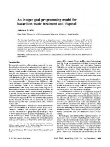
schedule reliability. An efficient network facilitates transshipments at terminals with high crane productivity and container capacity to minimise the cargo handling time. Transshipments are also used to get effective utilisation of vessel capacity such that the trunk lines are fed by several feeder lines and direct cargo along the trunk line. Finally, empty containers must be effectively balanced to ensure availability of containers. This is especially critical for reefer containers. Examples of different liner shipping networks are seen in Notteboom [21] summarized in figure 1.
C
H
B A
D
E
G
B A
F
(b) Hub-and-spoke network: A trunk line (D-E) and a set
(a) End-to-End connection
of direct feeder lines
C
I
B A
B
D
H E
A
(c) Line bundled
G
C F
(d) Main and feeder network- line bundled trunk lines and indirect feeder lines
Figure 1: Examples of routes and network desigs. Square nodes symbolise Hubs or main ports, whereas round nodes symbolize feeder ports.
Notteboom [21] argues that global liners are multi layered networks of different types since they are all competitive for particular circumstances. In practise any rotation and network configuration that makes sense from an economic and a market perspective is possible. 3.2.1. Value propositions A specific liner shipping company is referred to as a carrier, whereas the owner of a certain cargo is denoted a shipper. The competitive position of a carrier is a combination of port coverage, price, transit time, transhipments, schedule reliability, and over recent years corporate social responsibility of the company, where environmental friendly or “green” transport has received a lot of attention in recent years. The freight rate of transporting some cargo depends not only on the actual network cost, but also on the transit time, the container type needed (e.g. a refrigerating container), special regulations (restricted and dangerous goods), the number of transhipments, flag of the vessel(s), and naturally the relation between demand and supply for cargo transport on the connection in question. In addition the price covers the administrative overhead incurred 9
by the carrier comprising approximately 30 % of total cost [33]. Notteboom [22], Notteboom and Vernimmen [23] and Stopford [33] provide a qualifying discussion of pricing in liner shipping. The transit time is important because the interest on the value of the goods is paid by the shipper until the merchandise is delivered[22]. Furthermore, some goods are perishable and the time to market becomes crucial. The argumentation expands to a higher perceived market value of a product with a high reliability carrier, since this will reduce buffer stock requirements in a global supply chain. Corporate social responsibility for liner shippers is a very broad concept, which is hard to capture in a liner shipping network design model as a whole, but one important corporate social reliability is the environment, where the CO2 emissions of a carrier is significant. It is becoming increasingly important for companies to ensure transport with the lowest CO2 emission and hence slow steaming to reduce network bunker consumption and overall CO2 emission is a strong value proposition. Modelling and optimizing on liner shipping network design is a very capable tool for providing energy efficient network design simply by aiming to minimize bunker consumption. 3.2.2. Forecast and planning horizon A demand forecast for a given planning horizon is crucial to network design as the ideal network has a perfect fit between demand and capacity [33]. The demand for container transport fluctuates over a year with seasonal variance and peaks at certain times of year. These peaks may be regional, if they are related to a crop (e.g. bananas or lemons) typically transported over a short period, or global such as Christmas, where a large part of the world has an increased consumption of goods. Hence the network design is rarely stable over a yearly period. Some structure is fairly stable, but additional structure will reflect seasonality and hence the planning horizon for a network is important to the liner service network design and to the fleet deployment. General economic and financial conditions have a major impact on the liner service network design and fleet deployment, but are hard to predict compared to a seasonal pattern, which may be recognised and accounted for. 3.2.3. Schedule A schedule from the carriers’ point of view consists of a set of services with designated berthing times at a given frequency. As described it is generally assumed that each port call on a service has a weekly frequency and hence a service will arrive and depart at a given port on a certain weekday. The actual weekday may be crucial to customers in the desire to achieve a seamless supply chain. This also means that it might be crucial for a carrier to arrive at export ports before weekends and holidays to achieve seamless integration of the companies supply chains. The individual services are required to be good components of the network with regards to efficient transhipment facilities and fast direct services for critical connections. [21, 22] categorise a wide range of rotation patterns as follows:
10
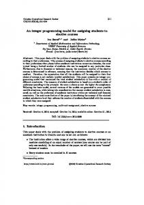
• End-to-End - a direct shuttle service between 2 ports. • Line Bundled - a rotation visiting a set of ports in a loop. • Trunk Lines - an end-to-end connection between hubs. • Direct feeder lines - shuttle from feeder port directly to a hub. • Indirect feeder lines - a line bundled rotation to a set of feeder ports and a hub. • Round-The-World (RTW) - a rotation following the equatorial belt visiting hubs in order to service the east-west and north-south trades in a grid. This type of string has a capacity constraint as it must traverse the panama canal restricted to panamax ships. • Pendulum - a service travelling back and forth like a pendulum i.e. Europe - Far East - US west cost - Far East - Europe. • Butterfly - Multiple cycles centered around one port. Each cycle visiting an alternating sequence of ports. One cycle may be a subset of another (see figure 2). • Conveyor Belt - a service connecting regional hubs designed for transshipments between continents at the crossing point of trade lanes.
u 5
u
u
3
4 6
2
u
7
1
u
u Figure 2: An example of a butterfly rotation
Rotation turnaround time varies from a single week up to 20 weeks although the average rotation is between 8-9 weeks. The rotation turnaround time is composed of voyage time at sea and the service time at ports used for piloting in to/out of the port, berthing and loading/unloading cargo. The number of port calls in a rotation is a trade-off between economies of scale and transit times [22]. High slot utilisation is achieved by collecting cargo at ports but transit times from the first port call to the last port call is incompetitive [22]. Another complicating factor is that port stays are very time consuming. In Notteboom [22] a COSTCO Europe-far east service is decomposed with regards to transit time and 21% of the transit time is the accumulated port stay. The schedule includes buffer time to account for delays due to weather, port congestions or exceeded terminal 11
handling time. These delays may cause speed increases on individual voyage legs which increases energy consumption and CO2 emission. The service is often divided into a fast head haul in an exporting direction, where the vessels have high capacity utilization and a slow back haul in the importing direction of trades, which due to trade imbalance tends to be under utilized. The trade imbalance and the fact that capacity is equal allows for marginal pricing for the shipper described in Stopford [33] page 552.
Figure 3: A Canada-Northern Europe service. Total round trip time is 28 days and to provide weekly frequency four vessels are sailing one week apart. The cargo headed for Europe is both destined for Europe, the Mediterranean and Asia. The latter two will transship in Bremerhaven to connect to appropriate services. Vice versa cargo headed for Canada has multiple origins.
3.2.4. Frequency As described in section 3.1 the liner shipping business is characterized by a public schedule. From the carriers point of view a schedule consists of a set of services. The services consists of a fixed itinerary of ports typically called with a weekly frequency [23, 33]. The fixed weekly frequency does introduce constraints on the network as opposed to varying frequencies of services. The fixed weekly frequency is widely used in container liner shipping due to significant planning advantages for carriers, shippers and terminals: • Reliability. Fixed departures enabling complete integration of customer supply chains. 12
Figure 4: Two connecting services. The Montreal service from figure 3 and a Europe-Mediterranean service with a round trip time of 2 weeks illustrated by two white vessels. The cargo composition on board vessels illustrate transhipments at the core of the liner shipping network design. The light blue incomplete service illustrates a larger service transporting cargo between Europe and Asia.
• Simplified network planning. A guiding rule for the carrier when designing the network. • Asset planning, the use of port berths and vessels can be planned for better utilization. • Planning routing scenarios Synchronization of connecting services may provide timely transhipments for critical connections. The success of containerization is the standardization of transport in containers of diverse products. The stable flow of general cargo in containers enables the carrier to maintain a weekly service. The weekly frequency of a schedule is achieved by assigning a number of vessels corresponding to a weekly dispersion on the trip at given speeds on each individual voyage between two ports (see figure 3 and 4). The speeds of each voyage between port pairs is thus closely related to the number of vessels. Therefore, adjusting the number of vessels on a service is a means to deciding on speeds. At the same time the decision of speed enables the carrier to adjust to demand fluctuation as he can increase capacity by increasing speed.
13
3.3. Assets and Infrastructure 3.3.1. Cost structure and economies of scale When minimizing the network cost we omit the administrative overhead estimated by Stopford [33] at 30 %. What is considered is the fixed asset costs and operational costs (OPEX) of operating a liner shipping network. The network cost of a carrier can be divided into fleet cost and cargo handling cost detailed below: • Fleet Cost: 1. Bunker Cost is the cost of bunker, which is the fuel deployed in container vessels. 2. Capital cost cost is the daily cost of a single vessel v. 3. Port Call Cost is a terminal fee for calling a terminal with a given vessel v. 4. Canal Cost is the cost of traversing a canal with a given vessel. 5. OPEX is the operating cost of a vessel including crew, maintenance and insurance. • Cargo handling Cost: 1. (un)load cost is the cargo handling cost at a given port. 2. Transhipment cost is the cost of transshipping a cargo in a port. 3. Equipment cost is the cost of owning / leasing containers. According to table 13.9 in Stopford [33] the bunker cost is between 35%-50 % of a vessels cost, Capital cost is 30%-45%, OPEX is between 6%-17% and port cost 9%-14%. Generally bunker cost exceeds capital costs apart from the largest vessels. Bunker consumption depends on the vessel type, the speed of operation, the draft of the vessel (e.g. the actual load), the number of operational reefer containers and the weather. Bunker consumption for a vessel profile is a cubic function [3, 33] and hence not easy to deal with seen from an integer linear programming perspective. During a round trip the vessel may sail at different speed between connections. The vessel may slow steam to save bunker or increase speed to meet a crucial transit time, or mitigate the threat of piracy. Speed may be constrained by hard weather conditions or navigation through difficult areas. This is a complicating aspect seen from a modelling perspective. The bunker cost is categorized as variable because the available sailing time is dependent on the port time, which again depends on load times of the cargo in question, delays and tidal waters. Both capital cost and OPEX varies with capacity. Economies of scale means that a large vessel is cheaper to operate per FFE [33]. The market rate of a vessel is called Time Charter Rate (TC rate) and represents the cost of leasing(chartering in) a container vessel into the fleet or for a carrier to forward lease(chartering out) an owned vessel to another carrier. The TC rate is as volatile as the market for general cargo. It fluctuates with seasonality and is highly dependent on 14
the length of the chartering period. A carrier may have an own fleet supplemented by chartering in and out to meet capacity requirements and to gain flexibility in asset management. TC cost will include daily running costs (OPEX) of the vessel, as crew costs, repair and maintenance. For vessels owned by the carrier the TC cost will cover OPEX and capital cost and depreciation of the vessels value (see [33] page 544). It is assumed that the TC costs represents a market rate, where the carrier will be able to forward lease the vessel in case of a surplus of vessels. The methods described herein will consider time independent TC costs, e.g. how to construct a network under fixed TC-costs, not considering financial asset management of a fleet of container vessels under an expected development of TC costs. For more details on such ideas see [6]. Port call cost and canal costs may be treated identically. The port call cost is a fee paid to the terminal. The fee depends on the size of the vessel i.e. the capacity booked in the terminal and also on the geographical location and size of the terminal. The canal costs may be found online for both the Suez and the Panama canal. The cost of traversing the Suez Canal depends on the Suez Canal Net Tonnage and whether the ship is laden. The Panama canal depends on the Panama Canal Universal Measurement System (PC /UMS) and the actual load of the ship. (Un)load and transhipment cost are also known as cargo handling costs. The load and unload costs are fixed once the cargo is selected for transport, but the transhipment cost depends on the routing of the product and hence the network design in the total number of transhipments. A global carrier will not provide direct connections for a significant percentage of the available transport scenarios, which incur transhipment at least once during a voyage. The cargo handling cost can be a non-linear piecewise function as some terminals have a price dependent on move thresholds and even a minimum number of moves. Equipment cost is the cost of containers. The carrier usually owns the majority of the containers used for cargo transport with the option of leasing in containers [33]. Equipment cost can be calculated as a daily cost based on the initial container cost, expected repair and maintenance cost divided by the expected lifetime of a container. Stopford [33] estimated the daily cost of a FFE dry container to 1 $ per day whereas a reefer FFE has a daily cost of 5.60 $. The transit time of a routing and the turn around time of equipment is decisive in how large an equipment fleet the carrier will need. Furthermore, trade imbalances means that carriers reposition empty containers. 3.3.2. Vessels An ocean going container vessel is the core part of a carriers’ operations. It can be characterized by specifications as FFE capacity, weight capacity, speed, length, width, draft, number of reefer plugs, ice class, age, engine, etc. The defining attribute is FFE capacity given as a nominal number. The actual capacity of a vessel depends on the service it is deployed to and the actual cargo on board.
The weight capacity of the vessel can similarly be considered by a nominal 15
number and a vessel cannot cater for more reefer containers than it has reefer plugs. As mentioned the draft, but also the air draft, length and beam of the vessel will dictate which ports, canals and straits the vessel can access, which again can be affected by the load on the vessel, tidal water and weather. Some waters have special access restrictions like the gulf of Finland which during winter requires ice class vessels for service. Though vessels are often built in series, in practice no vessels will have identical cost or performance (Stopford [33]) as the age and even the time since last hull scraping will affect performance. With regards to network design the vessels are grouped in vessel classes with similar properties such as capacity and speed interval eg. a PANAMAX vessel class denoting the maximal width for traversal of the Panama Canal. Other common groupings are according to a capacity band, i.e vessels with a nominal capacity of 1500-2100 TEU. Each vessel has a minimum Smin , and a maximum speed Smax , in knots. Besides a specific hull will usually have a design speed S ∗ , and design draft at which its design fuel consumption F ∗ , is optimized, the bulb at the stern of the vessel is part of this design. Still the actual speed largely decides the fuel consumption. Large vessels may use in excess of 200 metric tonnes (mt) of fuel per sailing day. Additional fuel is consumed by auxiliary engines for other vessel systems (1-12 mt/day) and for electricity for reefer units (a rule of thumb is 0.025 mt/day/100 reefers, depending on inside / outside temperature ) Calculating actual fuel consumption is very complex as vessel draft, wind, waves, currents and date of the last hull scraping will affect fuel consumption. The price of fuel, bunker, is generally proportional to the crude oil price and just as volatile.
Figure 5: Bunker index from march 2009- November 2010. Source: www.bunkerindex.com. The Bunker Index (BIX) is the Average Global Bunker Price (AGBP) for all individual port prices published on the Bunker Index website. The Bunker Index (BIX) is calculated by adding each individual daily port assessment price and dividing by the number of prices.
16
Figure 5 show the price fluctuation over 18 months. Large regional price differences exist, but the Average Global Bunker Price (AGBP) accounts for these fluctuations. Some seaboards are under sulphur emission restrictions, limiting the percentage of sulphur content in the bunker, denoted LSFO (Low Sulphur Fuel Oil, as opposed to High Sulphur Fuel Oil (HSFO)) is supplied with a premium to the bunker price and has reduced availability. The viscosity of the bunker also affect the price. Larger vessels are generally capable of burning bunker with higher viscosity at a cheaper price per metric ton. Diesel and Lubricants are required for running a vessel, but the costs are generally insignificant compared to the cost of bunker fuel. 3.3.3. Ports A port may consist of several terminals competing for the cargo traffic in the corresponding port. A carrier will typically use a single terminal at every port to facilitate connections between services. Ports have a maximum draft and the berths of a terminal have a maximum length. This results in vessel-port incompatibilities for some port-vessel combinations. A container ship is piloted in and out of port by a pilot employed at the port authorities. Some vessels may require more than one pilot to navigate into the port. To visit ports placed up river bassins like Hamburg and Antwerpen it may also be required to have tug boats to enter the river beds. Pilot times is the time it takes to be piloted in and out of a port. Pilot times may be several hours and for ports situated up a river bed it can be 8-10 hours. At most terminals a berthing slot is reserved in advance, whereas others serve vessels by a “first-come-first-serve (FCFS)” basis. A vessel may have to wait for a given pilot time or wait for an available berthing slot at FCFS ports. Congestion is not uncommon at terminals, this happens when a vessel is delayed due to contingencies as bad weather, slower cargo handling or more cargo than expected. This triggers a domino effect on the next vessels scheduled for the berth. In ports operating close to their operational capacity this can often be an issue that must be tackled. A vessel may have to wait for high tide to enter a port and may also not be able to leave a port upon low tide. A port call cost is paid to enter the port, which depends on vessel specifications. The port call cost covers cost to the pilots, tug boats, the port authorities and the terminal. Once the vessel has entered a terminal and moored to the berth, the vessel will commence unloading and loading of cargo. Cargo handling is often referred to as moves in general. Each move is associated with a cost to cover the cost of the cranes, terminal crew and terminal administration. Due to increased administrational work of exports and imports a transhipment move will typically be cheaper than a load and an unload move together. The carrier may have a contract on a fixed minimal number of moves at a given terminal, which is paid for in a terminal contract with a reduced cost on additional moves. These contracts are not easily dealt with in a mathematical programming context and we will assume a unit move and transhipment cost. Ports vary greatly in the number of moves they are able to perform during berth. This depends on the number of cranes and also the performance of the actual cranes and the 17
terminal infrastructure. The crane height and length of the terminal may also result in port-vessel incompatibilities as a vessel may not fit under a crane due to height and the crane length may not suffice to access all containers on deck. The number of moves a port is able to perform is denoted as its productivity. There is usually a distinction between main, transhipments and feeder ports. Feeder ports are usually small and their productivity may be varying according to the size and technical levels. Main ports mainly have a large quantity of import/export and some transhipment facility. Most main ports will have medium to high productivity. Lastly transhipment ports such as Balboa, Singapore and Algeciras do not have extensive import/exports but serve to tranship between services and intermodal transport. Transhipment ports compete on accessibility, price and productivity. As a result of this transshipment ports usually have a high productivity. Smaller ports may not have transhipment capability at all, due to lacking storage facilities for reefer containers or other lacking infrastructure. Vessels will replenish their bunker stock at port while cargo handling operations are working. This will be done by bunker-barges laying alongside the vessels, pumping the heavy bunker fuel onto the vessels. An operation that can take 10 hours or more for the largest vessels. Not all ports have bunker fuel suppliers, but main ports and transhipment port usually have suppliers. The price of bunker fuel is dependent on crude oil price, but the prices can vary greatly (20 % or more) on the same day in different ports (Plum and Jensen [26]). 3.3.4. Canals The two large canals of Panama and Suez enable fast transport between continents. To traverse the canals a significant fee is charged. The canals offer significantly faster transit times and also reduced operational costs due to the reduction of the sailing distance. Some sailing passages may have draft and width restrictions such as the Bosporus straight or Kiel Canal resulting in a significant detour for larger vessels. The current restriction on vessel size of the Panama canal is very decisive in the services serving the American east coast from the Far east and Austral Asia. No such restriction exists for the Suez canal with current container vessels. 3.3.5. Equipment Containers are generally available in lengths of: 20’, 40’, 45’ each of which exist in different types as: Dry, Refrigerating (reefers), open top and rack, plus additional specialized containers. A customer will generally require a specific type of container, though in some cases containers are used outside its designated scope, e.g. dry cargo in a refrigerating unit. Dry equipment covers roughly 80 % of a carriers equipment pool [33] with remainder mainly being reefers. There is a similar distribution on container sizes with around 80 % being 40’ containers Stopford [33]. Another restriction concerns the container itself and the nature of container transport. In order to transport goods in a container an empty container must be available to the shipper. Hence containers and in particular repositioning of empty containers to demand nodes is a particularity
18
of the container trade see [10, 19]. 3.4. Demand and Customers The goods and customers of containerized transports are plentiful and covers any type of manufactured goods, but can also be bulk-like cargo as stone, waste-paper or refrigerated commodities as fish or fruits. A service will usually focus on customers in a trade (sometimes multiple trades), this could be Asia to Europe or South America to North America. They may be grouped into east-west trades, which have larger volumes, allowing for economy of scale deploying huge vessels and into north-south trades, which have much refrigerated cargo requiring specialized vessels and faster transit time. Similarly all trades have special characteristics with regards to volume, service level requirements, etc. that governs, how a service can compete in the trade. 3.4.1. Demand In general the revenue of a cargo is closely related to the demand-supply balance, the demand being the volume of cargo to be transported and the supply being the capacity offered by container carriers. But many other effects play in. Specialized cargo, requiring specific equipment or different administrative handling will give higher revenue, for instance refrigerated or military cargo. As the demand is not symmetrical ( I.e. Asia exports much more than is imported) but the supply is ( Vessels return to Asia to be refilled). It follows that the revenue is not symmetric, which indeed is the case. Transporting a container from Asia to Europe can easily cost three times more than the reverse, even though the distance is identical ([4]). The production and consumption of some commodities vary over the year, some following harvest seasons, as fruit or fish, others following holidays and festivals as religious holidays or summer vacations. This gives variation in demand, some on a global level others only effecting a single port or trade. The biggest of these is Christmas which combined with other effects generates the yearly peak season in the third quarter, allowing European and north American warehouses to fill up prior to Christmas shopping. Another peak happens prior to Chinese new years, as Chinese factories exports their goods before closing down for the festivities. These demand fluctuations again effect the Revenues, with the highest revenues in the third quarter, but with variations over trades. A customer or shipper will usually only pay for a container transport once it is on the vessel or delivered, i.e there is no fee for booking and no fee for not submitting a cargo for a booking. This risk free booking policy for the shipper, causes many problems for the carrier and shipper: • It makes it hard to forecast the demand of cargo for some vessel departure, but since the capacity is a perishable resource (although it can be used at ports called later), the carrier will overbook departures, causing rollings of cargo, when forecasts and bookings short fall. • Shippers knows that such rollings is a risk, and to counter this they will intentionally book for more containers than they expect to ship, often spread at different carriers to optimize 19
flexibility. This especially happens in peak seasons as the third quarter, where capacities are the most pressed. Containerized transport has been a growth industry for many years, until 1985 yearly growth in demand was twice that of the world GDP growth. Since 1985 the demand has grown with 3 - 3.5 time that of the world GDP growth, giving growth rates of 8-10 % in most years. This has given an expectancy of growth in the industry. The delivery time of ordered vessels is several years and this makes the market slow to adapt to increased demand with resulting huge fluctuations in revenues as seen in the aftermath of the financial crisis. 3.4.2. Service level The specific service a customer is presented with, for transporting a container from port A to port B, the product, can be classified on a number of parameters: • The price, which is some basic rate, subject to additional fee’s and surcharges. • Bunker Adjustment Factor, a variable price component dependent on the bunker price. I.e. the carrier is sharing the risk of oil price volatility with the shipper. • Payment conditions, multiple exist explaining the details on responsibilities of seller, buyer and carrier. Some conditions require payment prepaid (CIF, when loading) others payment at collect (FOB). • Transit time, the time it takes for the container from A to B • Transhipments, the cargo is discharged in a third port C and loaded onto a new vessel. A direct non-transhipped product is preferred due to the increased risk of missing a connection and additional paperwork. • Frequency, a weekly service calling a port is preferred to a bi-weekly service due to increased flexibility. • Reliability, ocean carriers have large differences in how reliable services and product they operate. Reliability can be measured in a number of ways. • Paper work as documentation and administration, different carriers and products require different paperwork, adding complexity for the shipper. • Equipment, the carrier must supply the customer with a container prior to transporting. • Space, carrier must have space for the container, not rolling it for next week. • Weekday, some can be preferable to others. Vessels departing on a friday can be preferable to a departure on monday, as it can shorten the supply chain with three days (for a factory closed in the weekend). 20
All these factors can be relevant for a shipper, with price and transit time, often being the key factors. 3.4.3. Routing (Products) As a result of trade policies there are cabotage rules within countries. As such internal transport within the country may be restricted to routings on vessels flagged/owned/operated in the country. This also applies to transhipments of cargo destined within the country. Cabotage also applies for empty containers. Other special rules may exist, e.g. embargoes: when a country A is embargoing a country B, cargo from / to B can not be transshipped in A. (US/Iran). Dangerous goods are subject to IMO rules with regards to the quantity and the placement of these goods on the container vessel. 3.4.4. Competition & Partnerships As mentioned the economies of scale in liner shipping can give huge savings for larger volumes. This also motivates carriers to cooperate with competitors on operating services or subcontract to smaller operators. Such partnerships exists in various forms. Foreign Feeder. A service operating between a hub and a few proximate ports is called a feeder. These are usually operated by smaller vessels (less than 1250 FFE) and the cargo is originating / destined for the non-hub ports (or feeder ports) and transshipping in the hub to some ocean going service. Larger feeder ports (more than 300 FFE/week) can give the carrier the economy of scale to operate its own feeder service, but for smaller feeder ports it can be more attractive to subcontract this to a third party feeder operator. The feeder carrier will combine volume from different other global carriers to achieve economy of scale. The global carriers will get a lower and flexible cost on serving the ports of the feeder carrier in a pay per use deal, e.g. the global carrier will not commit to a fixed volume, but only pay for the actually transported cargo. Alliances and Vessel Sharing Agreements (VSA). The significant economies of scale achieved by deploying larger vessels is the motivation for multiple carriers to make a VSA. The concept is best illustrated by an example: Two carriers are operating identical services with a round trip time of six weeks, both deploying six vessels each with a capacity of 1000 FFE . A VSA combines the two services into a single service with the same rotation, same round trip time, but with six vessels each with a capacity of 2000 FFE . Each carrier owns three of the six vessels. The capacity of each of the six vessels is split 50-50 between the two carriers but the carriers both serve the ports with the same frequency and service level as before. Deploying and operating three large vessels as opposed to six smaller vessels presents a significant saving in operating cost for each carrier, see figure 13.11 in Stopford [33] without reducing the service levels presented to their customers. The VSA idea extends onto services where one carrier owns the majority of the capacity in terms of the 21
number of vessels. In practice VSA’s are complicated because the partners seldom have matching services and demand, available vessels etc., but VSAs are widely used and a central part of liner shipping. For more details on the mechanics of VSA’s refer to [2] and game theoretic observations on the subject. Slot Charter Agreements (SCA). is a combination of foreign feeders and VSA’s. One carrier will enter a contract to use capacity (slots) on another carriers service. This can either be on the full round trip of the service, allowing for the slot to be used differently in head and back haul, or on a specified part of the rotation. The contract will usually be for a fixed number of slots which is paid for used/unused, sometimes with an option for extra slots as pay per use. Other transport modes. Extraloaders are one time, often non-cyclic services which are executed to alleviate some unforeseen discrepancy between demand and capacity. This can be a huge build up of containers which can not get capacity on the planned network or a remedy of an empty container deficit in some region. Similarly cancellations occur if demand fails to materialize and capacity greatly exceeds demand. When considering the door to door supply chain of the containers, there will usually be one or more initial and final legs on other transport modes as Barges, Rail or Truck. In some cases the carrier will be responsible for these legs as well, carrier haulage as opposed to merchant haulage where the customer picks up the container at the terminal. As the cost of these intermodal legs are significant (The rail cost from Los Angeles to Chicago will exceed an ocean side cost from Shanghai to Los Angeles), these costs could be considered when creating a liner shipping network. 3.5. Qualifications of the benchmark suite data The literature review displays three important factors for the development of the benchmark suite: 1. The research community views the problem from different angles in terms of constraints and costs. As a consequence the data must cater for the important factors seen across the entire research field and also incorporate data on foreseeable extensions to current models. 2. A “base” model is needed in order to compare methods. 3. Currently, exact methods only solve very small instances, while heuristics such as the tabu search by Alvarez [5] caters for a large instance. As a consequence the benchmark suite should contain small, realistic instances, that may be solved to optimality within foreseeable future and large instances for heuristic development. The purpose of the benchmark suite is to provide data for prototype implementations of models and methods for the liner shipping network design and fleet deployment problem at a strategic level. The benchmark instances can be used to validate models and methods. 22
There are at least two pressing research questions in the LSNDP: efficient modelling of bunker consumption as a cubic function of speed and incorporating the level of service. Global carriers such as Maersk Line put a great effort into creating a network design of low bunker consumption to meet a demand for environmental friendly transportation of goods and improve the economy of the network. As noted by Notteboom and Vernimmen [23] the price of bunker has a significant impact on the network design and the fleet deployed. Therefore, formulas for bunker consumption based on vessel class are included in the benchmark suite to cater for calculations on the overall bunker consumption as a function of speed. At the same time Notteboom and Vernimmen [23] state that customers are demanding a high frequency and low transit times and therefore, level of service and competitive transit times are important factors in LSNDP. Due to the complexity of the LSNDP no known models of complete network design incorporates level of service or restrictions on transit time for specific commodities. The benchmark suite includes a set of maximal transit times on commodities in the benchmark suite as we believe level of service and transit time incorporation to be important open research questions in the liner service network design problem. The hardness of the problem is partly due to the large feasible solution space of rotations. Accounting for vessel class and port incompatibilities through draft, width and length of vessels is an opportunity to decrease the feasible solution space. The port data incorporates maximal draft and length. The vessel class data incorporates a single measure to express the draft, length and width of each vessel class. The draft measure is not variable with the cargo loaded which is an important limitation of the benchmark suite. The literature review show that the temporal aspect differs in the papers. We view the liner shipping network design problem separate from the actual operational schedule and hence do not incorporate any information on actual berthing windows or restrictions of frequency. It is, however, evident to us that the global carriers and the terminals in the industry generally adhere to the structure of a weekly frequency with few exceptions as noted by Notteboom and Vernimmen [23] and Stopford [33]. We have chosen to provide vessel data in terms of six fictitious, but realistic vessel classes, where multiple vessels share similar characteristics. We believe a global carrier has several similar vessels assigned to a service [1, 23, 5]. The domain of liner shipping is clearly very complex and rich on business specific details. A prototype implementation will contain the most important details, but omit details believed to be non-decisive for the conceptual understanding of the problem. Therefore, the benchmark suite does not cater for different equipment types such as reefer and high cube containers. The weight of vessels and cargo in particular are omitted from the benchmark instances. The benchmark instance will not flag the vessels in the data set as the actual vessel deployment is an operational issue. Likewise IMO rules apply to specific cargoes and stowage plans, which is out of scope of the considered LSNDP. The LSNDP is a mathematical model of a real life problem. In real life, weather has a large impact on the performance of a carrier, but weather is unpredictable, hard to forecast and very data
23
intensive. Therefore, weather is not considered in the benchmark instances. Additionally currents will affect travel times and energy consumption. Expanding the distances with information on currents is however out of scope for LSNDP. The benchmark instances are not meant for actual scheduling of services. Therefore tidal information on ports is not provided although they may be decisive for a specific berthing window at a port. On the same note the actual time stamp of demand availability is not included in the data of the benchmark suite. The following section will discuss data objects and data generation. A discussion on the range of instances needed to qualify the benchmark suite follows.
24
4. The benchmark suite for LNSDP The benchmark suite takes offset in publicly available data and past data for Maersk Line. External data sources are: • “Distances between ports - Pub. 151”, National Imagery and Mapping Agency [20] • The Hamburg Index, Vereinigung Hamburger Schiffsmakler und Schiffsagenten [37] • “Charter Rates 2000-2010”, Alphaliner [4] • “Container Freight Rate Insight”, Drewry Shipping consultants [11] The data from Maersk Line is from a given anonymous year and has been subject to reasonable random pertubation and anonymisation measures to protect the sensitivity and confidentiality of Maersk Line data. The purpose of the benchmark suite is to qualify algorithms for scalability, quality and robustness by providing realistic data for both the scale, structure and complexity of the liner shipping network design problem. We have chosen not to anonymise the actual ports to be able to evaluate the network from a business perspective, but the data still does not represent an actual business case, nor does it contain all relevant data. We hope the benchmark suite can be used to perform strategic analysis on various scenarios. The following section describes the data generation process in terms of the origin of the data and the logic used to derive the benchmark suite. For world instances demands are aggregated onto the main ports, see section 4.6.1 4.1. Data objects and data generation An instance consists of the following data: • Port list with port call cost as a function of vessel capacity • Fleet List with design speed and bunker consumption at design speed and idling • Distances • Demands The data items are illustrated in figure 6 giving an overview of the attributes of each item on a list. The benchmark suite will not dictate a planning horizon for the models at hand. However, a weekly frequency is a business standard [23, 25] and hence demand scenarios are based on weekly expectation. A week is easily scaled to longer planning periods if desired. The cost and revenues are not meant to reflect the actual cost of any carrier. The costs and revenues are constructed with care to reflect the relative cost structure within the network. This means that a large port is 25
Figure 6: Dataobjects of an instance
relatively cheaper to call than a small port. Likewise it is cheaper to transship a container in Asia than in Europe or the US. Revenues will reflect demand and supply such that visiting a distant port with low demand will require higher revenues per FFE than a central port with extensive own demand and supply. 4.2. Port List The port list specifies the ports in the instance and contains the following fields: • UNLOCODE (UNLO), 5-digit unique identifier for port [36] • Name • Country • Continent • Cabotage region if applicable • D region maps port to the revenue data supplied by Drewry Shipping consultants [11]
26
• Longitude • Latitude • Maximal berthing length • Maximal acceptable vessel draft • (Un)Load cost per FFE in USD • Transhipment cost FFE in USD. • Fixed port call cost • Variable port call cost as a function of FFE The port list reflects real ports ensuring that a solution can be mapped to a geographical coverage. This allows network planners and others without optimization background to evaluate a proposed network. UNLO
Name
Country
Cabotage
D reg
Longitude
Latitude
l
d
CNYAT
Yantian
China
China
China
114.27
22.58
370
16
p l
p ct
p C f
63
104
4680
c
c
p FFE 95
Table 2: Example of port entry. l is the length in metres of the maximal berth and d is the maximal draft. cpl is the (un)load cost and cpt the cost of a full transfer for transhipment. Cfp is the fixed port call cost and cpF F E is the port call cost as a function of capacity
The port call and cargo handling costs are based on Maersk Line data. All costs are perturbed randomly within a reasonable interval to protect the confidentiality of the data, while giving a realistic picture of the relative difference in cargo handling cost across geographical regions and terminal size and capacity. The transhipment cost will usually be lower than the sum of loading and discharging as transshipping does not require administrative paper work at the terminal in question. In an optimization model the load and discharge may be viewed as fixed costs once the demand is chosen for transport. The geographical location and the port size will determine a fixed cost for visiting the port and a variable cost related to the capacity of the vessel visiting the port. This relation is deduced experimentally from the perturbed Maersk Line data giving a non-zero fixed cost and a variable cost corresponding approximately to a linear function of the capacity. 4.3. Canal dues The canal dues for the worlds two most important canals; Panama and Suez, are included in the benchmark suite. These are based on their published cost structure [34, 24] and created for the relevant vessels classes. Additional canals are omitted from the benchmark suite.
27
4.4. Vessels Six generalized vessel classes are constructed from the fleet list of Maersk Line [7] representing realistic capacity classes in the network. A vessel class will contain the following information 1. TC rate per day per vessel in USD, this value includes OPEX, crew and maintenance costs. 2. Capacity in FFE 3. Design draft in metres 4. Minimal speed in knots 5. Maximal speed in knots 6. Design speed in knots 7. Daily bunker consumption at design speed 8. Own consumption when idling at ports 9. Number of vessels in the vessel class currently in the fleet 10. Panama canal fee 11. Suez canal fee The only size measure describing the vessels is draft. Others as length and beam width, should be seen as a proportional function of this. This generalization is done to simplify the problem, keeping in mind that a full description of the problem can extent to more than this one size measure without loosing applicability. Vessel class
FFE
Cv
d
Min s
Max s
s*
Fs ∗
F0
Q
PanamaFee
SuezFee
Feeder 450
450
4680
8
6
16
12
18.8
2.4
38
64800
175769.5
Feeder 800
800
7966
9.5
10
19
14
23.7
2.5
77
115200
218445
Panamax 1200
1200
11683
10
10
21
18
52.5
4
124
172800
267217
Panamax 2400
2400
21774
11
12
24
16
57.4
5.3
161
345600
413533
Post panamax
4200
33922
13
10
25
16.5
82.2
7.4
91
633007
Super panamax
7500
48750
12
10
24
17
126.9
10
10
1035376
Table 3: Example of the fleet list. Vessel class is the name of the class. FFE is the capacity in FFE . Cv is the TC rate. d is a single measure expressing width, length and draft for port/vessel comptibility. Min s, Max s is the speed interval of the vessel whereas s* is the design speed. Fs ∗,F0 are bunker consumption at design speed and idling respectively. Q is the available number of vessels in the fleet with these specifications. PanamaFee, SuezFee are the canal fees for the respective vessel classes
The fleet list will reflect the demand scenario of the instance as a trade lane has a smaller fleet than a world instance. 4.4.1. TC rates The TC rates fluctuate with the market and hence capturing TC rate is very dependant on the date it was retrieved as is seen from figure 7. We have compared data from Alphaliner [4] and “HAMBURG INDEX Containership Time-Charter-Rates” Vereinigung Hamburger Schiffsmakler
28
und Schiffsagenten [37], which have charter rates for vessels up to 4000 and 4800 TEU respectively1 . For vessel classes above 4800 TEU we have constructed a TC rate based on the percentual increase of TC rate in the Maersk Line data to corresponding capacity intervals of the fictitious vessel classes and have increased the Hamburg index of charter prices with the corresponding percentage.
Figure 7: Time charter rates based on the Hamburg Index for TC rates. Figure displayed with courtesy of VHSS, Vereinigung Hamburger Schiffsmakler und Schiffsagenten [37].
4.4.2. Bunker formulas Bunker cost is a significant cost component of the network. The bunker curves for the generalized vessel classes are based upon the formulas of Stopford [33], Alderton [3]. There is general agreement that bunker consumption, F , may be estimated by a cubic function F (s) = ( ss∗ )3 ∗F (s∗ ) for any speed, s, in the min speed and max speed intervals. This function disregards draft although it is a significant factor, so the bunker consumption should be the consumption at design draft as well. The design draft is the draft the vessel will have with an average load and for which it is designed to have the lowest bunker consumption as a function of speed. As noted by Alderton [3] the cube function is an estimation, which will be fairly accurate around the design speed, but 1 (http://www.vhss.de/containership
time-charter-rates eng.php)
29
will deviate significantly underestimating consumption at min speed and exaggerating bunker consumption at max speed. Alternatively polynomial interpolation to either a second or third degree polynomial can be achieved by plotting actual consumption patterns for target vessels of the generalized vessel classes. Fagerholt, Laporte, and Norstad [13] use a second degree polynomial, whereas Alderton [3] recommends a third degree polynomial. The deviation of the third degree polynomial is the more accurate, but as the vessel classes are generalized and many other factors affect bunker consumption, the deviation will differ for vessels within the class. Therefore, the cubic function will suffice as the data is representative and the bunker curves allow for optimization on speed and bunker consumption. The fleet list will specify the design speed and consumption at design speed for the cubic formula for each vessel class. The bunker price will be variable and the effect of bunker price could be a scenario for a user of the benchmark suite. Solutions submitted as best known solution or optimal solution should use an identical bunker price of 400 USD per ton. 4.5. Distances The distances are based on the National Imagery and Mapping Agency (NIMA, 2001). The data from NIMA contains distances from each port to major way points and ports in the vicinity. The data enables a mapping of global sailing routes onto a graph of ports and way points. Each arc is given specifications such as the maximal draft and maximal width such as the panama canal, which has a width restriction. A single-source shortest path algorithm between each pair of ports determines the shortest feasible path for each vessel class based on this data. It means that the distance between Oakland on the US West Cost and Savannah on the US East Coast will differ for vessels able to traverse the Panama canal as opposed to vessels not able to traverse the Panama canal. To cater for canal cost a distance will indicate whether the distance is based on a visit to the Suez Canal and/or the Panama canal. The distance file is a table with multiple entries for each port pair depending on draft limitations and canal usage. We assume symmetric distances i.e. that the distance from A to B is equal to the distance from B to A. • Port A • Port B • Distance • Draft limit • Panama Canal? • Suez Canal?
30
O
D
Nautical miles
draft limit
Suez canal
Panama canal
GBABD
USOAK
7953
12
No
Yes
GBABD
USOAK
13862
No
No
Table 4: Example of distance file. O is the origin UNLOCODE, D the destination UNLOCODE. draft limit is in metres and canal traversal for Panama and Suez is denoted for each distance to calculate canal fees
4.5.1. Distance generation The distances between ports is generated using the data from the National Imagery and Mapping Agency which are the highways at sea consisting of actual ports and ocean junctions called way points, which are used to navigate. By manual inspection of the distances central distances where identified to be erroneous. It has been attempted to verify the correctness of several distances thorugh external data sources correcting obvious errors in National Imagery and Mapping Agency [20] but the distances are not guaranteed to be the shortests distance due to the selection of waypoints and undetected errors in the data from National Imagery and Mapping Agency [20]. The distances have been collected and put into a graph G = (V, E). The set of ports P and S the set of way points W constitute V = P W . The edge set E are from National Imagery and Mapping Agency [20]. Two distance files are generated 1. An all-to-all distance matrix for the port set P 2. A graph of the instance G = (V, E) The graph file will contain all vertexes and edges needed to navigate between any pair of the ports in P with the fleet F . The files are generated using a shortest path algorithm between all pairs of ports for each vessel class in the fleet F . The distances are generated for the distance matrix and every edge used in any shortest path along with its endpoints are included in the graph of the instance. 4.6. Demands Realistic demand data with regards to the asymmetric world trade is important as this is the complicating matter, when deciding on capacity and port sequences. A maximal transit time for each demand is provided for future models incorporating level of service or maximal transit time constraints. The demand table contains the following information: • Origin port • Destination port • Quantity in FFE • Freight Rate
31
Source
Destination
Quantity FFE
Freight rate/FFE
Max. transit time
USLSA
CNYAT
370
1500
15
Table 5: Example of demand file. Source and Destination ar egiven as UNLOCODES and the maximal transit time is measured in days
• Maximal transit time The demands are assumed to be the expected weekly demand. 4.6.1. Data generation of demands The demands for an instance are based on Maersk Line data. The demand volumes are perturbed randomly within a reasonable interval to protect the confidentiality of the data while giving a realistic picture of the world trade with regards to import and export volumes of regions. Upon a selection of P ′ ⊂ P the demand can be generated by several aggregation strategies: 1. Do nothing - All direct demands within P ′ . 2. Feeder mapping - all feeder ports in the vicinity of P ′ is mapped onto the nearest main port q ∈ P ′. 3. Trade Lane mapping - ports in adjacent regions transhipping to the Trade Lane is mapped onto the nearest transhipment port in P ′ . 4. External mapping - all demand pairs with either origin or destination in P ′ is mapped onto the nearest transhipment port in P ′ .. 5. Aggregation of trade volumes. Having direct demands only is a rather limited and unrealistic demand picture due to the large proportion of transshipped demands, but may be seen as experimental instances. A feeder mapping is fairly realistic for the world instances, but very limited for the trade lane instances. The external mapping is extensive as it should result in a realistic volume scenario within the instance with respect for the origin/destination of demands being fixed by the instance. To minimize the number of distinct OD demands an additional aggregation method may be applied to collect volumes below some threshold. For the instances in the benchmark suite we have applied a combination of feeder, trade lane and external mapping. The revenues are based on the trade lane prices found in “the container freight rate index”, with courtesy of Drewry Shipping consultants [11], www.drewry.co.uk. The rates are independent of any carrier and contains reliable market data collected across several carriers and markets. Drewry Shipping consultants [11] does not contain South America West coast and some region pairs and where possible the official rates from the website of Hapag-Lloyd has been applied. The market freight rates will be subtracted the administration overhead as we are only dealing with the network cost and the profitability of the network. This is estimated to 30% by Stopford [33]. The volume 32
of the origin/destination ports along with the distance to the nearest main or transhipment port are used to vary the trade lane price according to the demand structure, such that a demand from a transhipment/main port is cheaper than a demand from a feeder port and feeder port revenues are dependent on the distance from the main port. Lastly, the freight rates are perturbed within an interval of +/-5% to reflect price variance of different markets and cargoes.
5. Instance range of the benchmark suite The instances are meant to challenge both exact and heuristic methods. Exact methods are currently limited to approximately 10 ports, where the tabu search of Alvarez [5] provides heuristic results for 120 ports. Furthermore, the instances are meant to encourage the progress of method development and hence include instances of real life scale although we cannot yet accommodate solving them to optimality. Some of the instances are subsets of a larger network, where the subset is selected to highlight various aspects of the LSNDP, this could be under capacitated, over capacitated, single hub, multiple hub or draft restricted instances. The provided instances and their origin is listed below: • Trade lane instances. Demands are based on feeder and trade lane mapping. 1. Pacific (Asia-US West) 2. EuropeAsia Europe, Middle East and Far east regions • Single Hub instances. Demands are based on feeder and external mapping. 1. WAF West Africa with Algeciras as hub to West African ports. 2. Baltic Baltic sea with Bremerhaven as hub. • World Instances. Demands are based on feeder mapping as all regions are present in the instances. 1. Small 47 Main ports worldwide identified by Maersk Line 2. Large 197 ports - the majority of ports serviced by Maersk Line directly. The Pacific and the single/multiple hub instances will be challenging for the exact approaches and will also be applicable to model development as the models can be verified analysing the results of the benchmark suite. The EuropeAsia trade lane instance and world instances will be challenging for the heuristics developing new methods, neighborhoods and competing for the current best known objective value. Exact methods solving these instances to optimality is not expected in the near future. We will not provide computational results for the large world instance as the size is currently considered out of scope even for heuristic methods. 33
Ports P ′
Demands
Pacific
45
722
EuropeAsia
111
4000
Baltic
12
22
Waf
19
38
Small
47
1764
Large
197
9630
Instance
Table 6: The instances of the benchmark suite with indication of the number of ports and the number of distinct demands
34
6. Model Constants in the model • v ∈ V , is the finite set of vessel classes considered. • s ∈ S, a rotation is a cyclic rotation of vessels, all of the same vessel class, Vs . Port calls are assumed with weekly frequency. • CVs Capacity of a vessels class V used by rotation s • p, q ∈ P , the set of ports. • X, Y ∈ R, the set of regions, each consisting of a set of ports, X = {p1 , . . . , pn }. A port is a member of at least one region. • dXY , possible number of containers to transport from region X ∈ R to region Y ∈ R. daY is the exports from port a to region Y and dXb the imports from region X to port b. The demand dXY represents the previously mentioned trade terminology, a combined representation of cargo, i.e Europe to South America. These can as such use overlapping regions, i.e another trade could be Asia to West Coast South America, depending on the necessary level of detail. • cpv , the cost for vessel class v to service port p. • up The cost to load, unload or half the cost of transhipping, one unit of flow in port p. • saY , sXb , respectively the revenue of a origin load of one unit from port a to region Y , or a destination unload of one unit from region Y to port b • tpqs = distanceqp · Kvs the travel cost between ports p and port q for rotation s. Where Kvs is the cost per nautical mile of deploying vessel class v. • Mp is the set of maximum number of calls for any rotation to port p. • Nv is the set of maximum number of ports a vesselclass v may visit. • Epvs ∈ {0, 1} is set iff vs is not draught restricted in p • gpXY ∈ {0, 1} is set iff p allows for transhipments of XY . • wpv is the number of container moves pr hour of vessel class v in port p. w˜pv is transformed to the impact on cost / distance. • DSDv is the weekly distance covered by a vessel of class v. • distanceqp , the distance in nautical miles from port q to p. 35
Variables in the model: XY • 0 ≤ Ukps ≤ M AX(dXY · gpXY , dXp |p ∈ Y ) The amount of containers from region X to region
Y unloaded in port p by rotation s on the k’th visit. XY • 0 ≤ LXY · gpXY , dpY |p ∈ X) The amount of containers from region X to region kps ≤ M AX(d
Y loaded in port p by rotation s by rotation s on the k’th visit.. vs • xkh pqs ≤ Ep , 0 − 1 variable which indicate if rotation s sails between port p and port q.
• zspY , zsXp 0 − 1 variable which indicate if the containers from region X to region Y is transported on rotation s XY • fkps ≤ dXY The amount of XY -containers carried on rotation s in port p on visit k.
The mathematical model then becomes: max
X X X
(
X
saY · LXY kas +
k∈Mp s∈S XY ∈K a∈X
−
X
p∈P
−
up
X
X X
k∈Mp XY ∈K s∈S
XXX
cps + tpqs
p∈P q∈P s∈S
X
(1)
b∈Y XY (LXY kps + Ukps )
(2)
X X
(3)
h∈Mq k∈Mp
36
XY sXb · Ukbs )
xhk qps
X X
XY pY (LXY kps − Ukps ) ≤ d
∀p ∈ X, ∀XY ∈ K
(4)
XY Xp (Ukps − LXY kps ) ≤ d
∀p ∈ Y, ∀XY ∈ K
(5)
∀XY ∈ K
(6)
∀p ∈ P \ {X, Y }, ∀XY ∈ K
(7)
∀v ∈ V
(8)
zspY ≤ 1
∀p ∈ X, ∀XY ∈ K
(9)
zsXp ≤ 1
∀p ∈ Y, ∀XY ∈ K
(10)
∀p ∈ P, ∀k ∈ Mp , ∀s ∈ S
(11)
∀p ∈ P, ∀k ∈ Mp , ∀s ∈ S
(12)
xhk qps ≤ 1
∀p ∈ P, ∀k ∈ Mp ∀s ∈ S
(13)
xkh pqs ≤ 1
∀p ∈ P, ∀k ∈ Mp ∀s ∈ S
(14)
pY LXY · zspY + gpXY (dXY − dpY ) kps ≤ d
∀p ∈ X, ∀XY ∈ K, ∀s ∈ S
(15)
XY Ukps ≤ dXp · zsXp + gpXY (dXY − dXp )
∀p ∈ Y, ∀XY ∈ K, ∀s ∈ S
(16)
s.t 0 ≤
k∈Mp s∈S
X X
0≤
k∈Mp s∈S
X X X
XY (LXY kps − Ukps ) =
p∈X k∈Mp s∈S
X X X
XY − LXY (Ukqs kqs )
q∈Y k∈Mp s∈S
X X
XY (LXY kps − Ukps ) = 0
k∈Mp s∈S
XXX X X
(distanceqp · xhk qps
s∈v p∈P q∈P h∈Mq k∈Mp
X
+ X
XY v w˜pv (LXY kps + Ukps )) ≤ |v| · DSD
XY ∈K
s∈S
X s∈S
X
XY fkps ≤ CVs ·
XY ∈K
X X
q∈P h∈Mq
X X
X X
xhk qps
q∈P h∈Mq
xhk qps −
X X
xkh pqs = 0
q∈P h∈Mq
q∈P h∈Mq
X X
q∈P h∈Mq
X
k∈Mp
X
k∈Mp XY XY XY XY xhk qps = 1 =⇒ fkps = fhqs + Lkps − Ukps
∀XY ∈ K ∀p ∈ P, ∀q ∈ P
X X p∈P k∈Mp
LXY kps =
X X
XY Ukps
∀k ∈ Mp , ∀s ∈ S
(17)
∀s ∈ S, ∀XY ∈ K
(18)
p∈P k∈Mp
(19) The objective (1) to (3) is divided into four terms. The revenue of container transport, the expenses from port calls, the cargo handling expenses including transhipment cost and finally the estimated vessel and fuel cost for the rotations. Constraints (4), (5), (6) and (7) ensures load balance on a rotation for port exports, imports and between regions. A limited number of each 37
vessel class is available (8) based on the weekly frequency constraint. (9) and (10) ensures that a commodity is served at most once. Constraints (11) ensures that a rotation does not exceed its capacity at departure from a port. Cyclic rotation are ensured by (12) Constraint (15) and (16) ensures unsplit service of a commodity and (17) sets the flow variables. Routings must adhere to cabotage restrictions (21), All flowed demand must consider its transittime (22).
Subtoureliminationonxhk qps
(20)
Cabotage
(21)
T ransittime
(22)
M aximalnumberof P ortcalls
(23)
P redef inedStartP orts
(24)
Subtour elimination is done by (20).
38
7. Conclusion and future work In conclusion the LSNDP is a complex optimization problem where operations research has huge potential for making energy efficient and competitive liner shipping networks to the benefit of all stakeholders. The literature review reveals a young research field, where the scope and domain of LSNDP is discussed. Computational results are based on data sets generated by the authors with more or less details and hence comparison of methods and models is not currently possible. This paper brings together literature on operations research and business economics of liner shipping. It shows that fuel is the dominant cost in liner shipping and hence surging fuel prices makes slow steaming sustainable for liner shipping companies provided that they can maintain competitive transit time of products. The latter is an open research question for liner shipping network design. A thorough discussion of the business domain of liner shipping seen in relation to mathematical models of the LSNDP is provided with valuable input from Maersk Line, one of the worlds major global carriers. The domain discussion highlights market conditions, business constraint and cost structures of a real life liner shipping network. A benchmark suite in the form of six data instances is made available upon request. We have discussed in depth the content of the data objects and the generation of cost structures and constraint structures with offset in data from Maersk Line, Drewry Shipping consultants [11], Alphaliner [4], Vereinigung Hamburger Schiffsmakler und Schiffsagenten [37] and National Imagery and Mapping Agency [20] to ensure a set of data instances with close resemblance to real life. The data instances are not real life cases, but the cost structures and market structures of demand and revenues should be present to reflect real life liner shipping networks. Future work will be to test the benchmark instances using the tabu search of Alvarez [5] to verify the data and provide a set of non-optimal best known solutions for the benchmark suite. It is our hope that the benchmark suite will become the solomon instances of LSNDP motivating researchers to engage with the field of liner shipping network design. The benchmark suite will be available as an svn repository. Please contact the corresponding author for access.
39
[1] R. Agarwal and O. Ergun. Ship scheduling and network design for cargo routing in liner shipping. Transportation Science, 2008. [2] R.
Agarwal
game
in
– 524,
and
service 2008.
O.
Ergun.
network
Mechanism
alliances.
ISSN 0167-6377.
design
Operations doi:
for
a
multicommodity
Research
Letters,
DOI:10.1016/j.orl.2008.04.007.
flow
36(5):520 URL
http://www.sciencedirect.com/science/article/B6V8M-4SR711J-6/2/c58db3dc7872a268246404f3b7b7e284. [3] P. Alderton, 2005. [4] Alphaliner. Alphalinercharter rates 2000-2010, 2010. URL http://www.alphaliner.com. [5] J. F. Alvarez. Joint routing and deployment of a fleet of container vessels. Maritime Economics and Logistics, 11(2):186, 2009. [6] Jose Fernando Alvarez, Panagiotis Tsilingiris, Erna Engebrethsen, and Nikolaos M. P. Kakalis. Robust fleet sizing and deployment for industrial and independent bulk ocean shipping companies. INFOR, Special Issue on Maritime Transportation. [7] A.P. Møller-Mærsk Fleet List 2008. A.p. møller-mærsk fleet list 2008. [8] Pierre Cariou. Is slow steaming a sustainable means of reducing co2 emissions from container shipping? [9] M. Christiansen, D. Ronen, B. Nygreen, and K. Fagerholt. Maritime transportation. Handbooks in Operations Research and Management Sciences, 14:189–284, 2007. [10] J.-X. Dong and D. Song. Container fleet sizing and empty repositioning in liner shipping systems. Transportation Research Part E: Logistics and Transportation Review, 45(6):860– 877, 11 2009. [11] Drewry
Shipping
consultants.
Container
freight
rate
insight,
2010.
URL
http://www.drewry.co.uk/publications/view_publication.php?id=358. [12] K. Fagerholt, T. A. V. Johnsen, and H. Lindstad. Fleet deployment in liner shipping: A case study. Maritime Policy and Management, 36(5):397–409, 2009. [13] K. Fagerholt, G. Laporte, and I. Norstad. Reducing fuel emissions by optimizing speed on shipping routes. The Journal of the Operational Research Society, 61(3):523–529, 08/19 2009. URL http://dx.doi.org/10.1057/jors.2009.77. [14] Kjetil Fagerholt. Designing optimal routes in a liner shipping problem. Maritime Policy & Management, 31(4):259 – 268, 2004. doi: 10.1080/0308883042000259819.
40
[15] S. Gelareh and Q. Meng. A novel modeling approach for the fleet deployment problem within a short-term planning horizon. Transportation Research Part E: Logistics and Transportation Review, 46(1):76–89, 1 2010. [16] S. Gelareh, S. Nickel, and D. Pisinger. Liner shipping hub network design in a competitive environment. Transportation Research Part E: Logistics and Transportation Review, 46(6): 991–1004, 2010. [17] A. Imai, K. Shintani, and S. Papadimitriou. Multi-port versus hub-and-spoke port calls by containerships. Transportation Research Part E: Logistics and Transportation Review, 45: 740–757, 2009. doi: doi/10.1016/j.tre.2009.01.002. [18] M.G Karlaftis, K. Kepaptsoglou, and E. Sambracos. Containership routing with time deadlines and simultaneous deliveries and pick-ups. Transportation Research Part E, 45:210–221, 2009. doi: 10.1016/j.tre.2008.05.001. [19] B. Lø fstedt, D. Pisinger, and S. Spoorendonk. Caper - the cargo allocation problem with empty repositioning. Accepted for INFOR - special issue on maritime transportation, 2010. [20] National Imagery and Mapping Agency. Distances between ports - pub. 151, 2001. URL http://www.marcon.com/library/resources/DBP/DBP.html. [21] T.E. Notteboom. A carriers perspective on container network configuration at sea and on land. Journal of International Trade and Logistics, 2(1):65–87, 2004. [22] T.E. Notteboom. The time factor in liner shipping services. Maritime Economics and logistics, 8:19–39, 2006. [23] T.E. Notteboom and B. Vernimmen. The effect of high fuel costs on liner service configuration in container shipping. Journal of Transport Geography, 17(5):325–337, 9 2009. [24] Panama Canal. The panama canal. URL http://www.pancanal.com/eng/maritime/tolls.html. [25] Personal communication with Maersk Line. Network and product at maersk line. [26] Christian E. M. Plum and Peter Neergaard Jensen. Minimization of bunker costs. Master’s thesis, 2007. [27] B. J. Powell and A. N. Perakis. Fleet deployment optimization for liner shipping: an integer programming model. Maritime Policy and Management, 24(2):183–192, 1997. Cited By (since 1996): 17. [28] K. Rana and R.G. Vickson. Routing container ships using lagrangian relaxation and decomposition. Transportation Science, 25(3):201–214, 1991. 41
[29] L. B. Reinhardt and B. Kallehauge. Network design for container shipping using cutting planes. In Conference on Maritime & Intermodal Logistics, Singapore, December 2007. [30] D. Ronen, K. Fagerholt, and M. Christiansen. Ship routing and scheduling: Status and perspectives. Transportation Science, 38(1):1–18, 2004. doi: 10.1287/trsc.1030.0036. [31] K. Shintani, A. Imai, E. Nishimura, and S. Papadimitriou. The container shipping network design problem with empty container repositioning. Transportation Research Part E: Logistics and Transportation Review, 43(1):39–59, 2007. doi: 10.1016/j.tre.2005.05.003. [32] Marius M. Solomon. Algorithms for the vehicle routing and scheduling problems with time window constraints. Operations research, 35(2):254–265, Mar 1987. [33] M. Stopford, 1997. [34] Suez. Suez canal authority. URL http://www.suezcanal.gov.eg/calc.aspx. [35] TheWorldShippingCouncil. The liner shipping industry and carbon emissions policy. 2009. [36] UNLOCODE.
United
nations
economic
commission
for
europe.
URL
http://www.unece.org/cefact/locode/. [37] Vereinigung Hamburger Schiffsmakler und Schiffsagenten. The hamburg shipbrokers’ association. URL http://www.vhss.de/contex.php.
42
Operations research within liner shipping network design is scarce compared to other modes of transportation. The problem is a complex optimization problem and requires profound knowledge of the domain and data sources. It is believed that there are many entry barriers to the domain and data for liner shipping network design. In this paper we present a thorough description of the liner shipping domain applied to network design along with an integer programming model based on the services that constitute the fixed schedule of a liner shipping company. The model presented is very rich and may be relaxed as well as decomposed. A benchmark suite of data instances is discussed along with data generation and sources of data to reflect the business structure of a global liner shipping network. The paper is motivated by providing easy access to the domain and the data sources of liner shipping for operations researchers in general. Future work is to generate an actual set of data instances and provide computational results for the instances.
DTU Management Engineering Department of Management Engineering Technical University of Denmark Produktionstorvet Building 424 DK-2800 Kongens Lyngby Denmark Tel. +45 45 25 48 00 Fax +45 45 93 34 35 www.man.dtu.dk