An Integrated Model of Cognitive Control in Task Switching

Psychological Review 2008, Vol. 115, No. 3, 602– 639

Copyright 2008 by the American Psychological Association 0033-295X/08/$12.00 DOI: 10.1037/0033-295X.115.3.602

An Integrated Model of Cognitive Control in Task Switching Erik M. Altmann

Wayne D. Gray

Michigan State University

Rensselaer Polytechnic Institute

A model of cognitive control in task switching is developed in which controlled performance depends on the system maintaining access to a code in episodic memory representing the most recently cued task. The main constraint on access to the current task code is proactive interference from old task codes. This interference and the mechanisms that contend with it reproduce a wide range of behavioral phenomena when simulated, including well-known task-switching effects, such as latency and error switch costs, and effects on which other theories are silent, such as with-run slowing and within-run error increase. The model generalizes across multiple task-switching procedures, suggesting that episodic task codes play an important role in keeping the cognitive system focused under a variety of performance constraints. Keywords: cognitive control, task switching, cognitive simulation, episodic memory, executive function

Questions about how people set, focus on, and switch among the short-term goals that govern everyday behavior are key issues in the domain of cognitive control.1 A number of experimental paradigms touch on this kind of control—including, at different levels, puzzle solving and the psychological refractory period— but the one most closely associated with the behavior of interest here is task switching. In a procedure of particular interest here, which we term the randomized-runs procedure, the experimental participant performs a large number of trials in sequence. Each trial involves presentation of a simple stimulus—a randomly selected digit, in the most common materials—to which the participant responds by judging whether the digit is even or odd (one task) or higher or lower than five (the other task), depending on which task is currently correct. Figure 1 shows the timeline of events in this procedure. Every few trials, a task cue is presented briefly and then withdrawn, after which the participant performs that task for the subsequent run of trials, until the next cue is presented. The cues themselves are randomly selected, such that on “switch” runs, the task is switched from what it was on the previous run, whereas on “repeat” runs, the task is the same as it was on the previous run. With the task changing frequently, accurate performance depends on maintaining some kind of mental representation of the task to perform now. The idea with this procedure is to distill some of the essence of the “what did I want now that I’m here?” problem associated with simple errands, for example; one sets out to fetch something, having fetched many similar things before, and the old things interfere— or one’s mind simply wanders. How the system

responds to this mundane cognitive-control challenge is what we would like to understand in theoretical terms. At this level of everyday situations, it seems useful to distinguish the one we sketched above from others that may be evoked by the term “task switching.” One such situation is task interruption (Van Bergen, 1968; Zeigarnik, 1938). If someone is working on a project—a manuscript, for example—and is interrupted by a phone call, there can be a cost associated with reconstructing the mental context that was active when the interruption occurred (Altmann & Trafton, 2007; Hodgetts & Jones, 2006). Such interruptions make an attractive conceptual frame for task-switching studies (e.g., Monsell, 2003), yet the costs of switching between tasks that involve some reasonable amount of cognitive state, such as working on a manuscript and talking to someone, may be driven by operations on fairly rich knowledge representations (Altmann & Trafton, 2007). In task switching, the representations that support performance are much leaner, and the interruptions are much more frequent, such that behavioral measures may index rather different mechanisms. A second situation evoked by task switching is multitasking, such as when someone drives a car while interacting with a navigation system or a passenger (or a caller on the phone). In an environment like this, in which one or both tasks are continuous, an important constraint is that task switches have to be scheduled such that neither task starves for attention (e.g., Salvucci & Taatgen, 2008). Thus, both task interruption and multitasking involve control processes beyond those that keep the system focused on a small but frequently changing unit of control information. Nonetheless, the latter would seem to be a substrate on which more complex expressions of cognitive control are built. Indeed, the computational mechanisms we describe here are adapted from a model of puzzle solving (Altmann & Trafton, 2002) in which cognitive control involves suspending and activating subgoals to control search through a problem space. The

Erik M. Altmann, Department of Psychology, Michigan State University; Wayne D. Gray, Cognitive Science Department, Rensselaer Polytechnic Institute. This work was supported by Office of Naval Research Grants N0001403-1-0063 and N00014-06-1-0077 to Erik M. Altmann and N00014-03-10046 and N00014-07-1-0033 to Wayne D. Gray and by Air Force Office of Scientific Research Grants F49620-03-1-0143 and FA9550-06-1-0074 to Wayne D. Gray. Correspondence concerning this article should be addressed to Erik M. Altmann, Department of Psychology, Michigan State University, East Lansing, MI 48824. E-mail: [email protected]

1

The authors thank Gordon Logan, Nachshon Meiran, Nick Yeung, and two anonymous reviewers for their detailed and thoughtful comments on this article, and Alan Allport and Rich Carlson for formative comments on an earlier version. 602

COGNITIVE CONTROL MODEL

603

Figure 1. Timeline of events in the randomized-runs task-switching procedure used in Simulation Study 1, showing three consecutive runs of trials.

commonality is that accurate performance again depends on the system having access to the correct subgoal at the correct time in a situation in which the subgoal changes frequently. An active task-switching literature has grown up over the past dozen years or so, shaped by three roughly contemporaneous studies that focused on trying to explain the costs of switching between simple tasks. Allport, Styles, and Hsieh (1994) proposed that these switch costs were linked directly to carryover effects from previous performance, a construct they termed “task-set inertia” and likened to proactive interference. This proposal first illustrated the approach that we continue here of analyzing control processes in terms of familiar memory constructs (interference, priming, etc.; Altmann, 2003). Rogers and Monsell (1995), in contrast, assumed that switch costs reflected processes dedicated specifically to cognitive control—processes that, figuratively,

were the “little signal person in the head” (p. 217) throwing a switch that would then send the cognitive train of thought down the correct track. This has come to be known as the “reconfiguration” metaphor and remains under active consideration today (e.g., Steinhauser, Maier, & Hubner, 2007). Finally, Meiran (1996) began to bridge these two approaches, suggesting that both carryover effects from the previous trial and reconfiguration processes were at work. These three original studies (see also Fagot, 1994) triggered a widespread interest in trying to explain switch costs, although success with this has been limited to some extent by construct validity problems (Altmann, 2007a). One of our goals is to illuminate these problems by simulating performance in different procedures with one set of control mechanisms so as to map different switch costs to different origins. A broader goal is to show that switch costs themselves are only part of a larger empir-

604

ALTMANN AND GRAY

ical landscape that, viewed as a whole, offers reasonably strong constraints on models of cognitive control in task switching. We start with the premise that each time the system is presented with a task cue, it encodes a new representation of this cue in episodic memory. We then ask what kinds of control processes the system might have to deploy to maintain access to the current code created by this process, given proactive interference from old codes created by this process in response to previous cue presentations. This analysis yields a blueprint that we develop into a computational model in which proactive interference builds up in the course of simulated performance. This proactive interference and the mechanisms that contend with it reproduce a variety of response-latency and error effects, some well known and widely interpreted and some less so. We constrain our theoretical approach by aiming for four types of integration. First and foremost is functional integration, meaning that each central mechanism in our model plays some functional role in the model’s performance, with some other mechanism(s) depending on or affected by its output. Second and related is empirical integration, meaning that we use the model to argue that empirical effects that on the surface might seem to be completely unrelated are in fact related in terms of underlying mechanisms. Third is theoretical integration, meaning that we assemble the model largely from existing cognitive constructs rather than developing new ones. Fourth is procedural integration, meaning that we show that one set of mechanisms can account for performance in multiple task-switching procedures, including the two used in the bulk of studies that make up the task-switching literature. The article is organized as follows. In the first two sections, we describe our cognitive control model (CCM) at its abstract and computational levels. At the abstract level, we build on previous work (Altmann, 2002; Altmann & Gray, 2002) to make a new prediction. At the computational level, we describe a model that reproduces latency and error measures based on performance of full-length simulated experimental sessions. We then present three studies demonstrating the functional sufficiency and explanatory scope of this computational model. In Simulation Study 1, we fit data from a new experiment that integrates a suite of relevant effects in one design, some replicating previous work and some testing new questions. In Simulation Studies 2 and 3, we apply the model to published data from the two most common taskswitching procedures— explicit cuing and alternating runs—to show that it generalizes beyond situations in which memory for the most recent task is an explicit performance requirement. In Simulation Study 2, we also develop an account of a widely reported interaction of cue-stimulus interval (CSI) and switching, and in Simulation Study 3, we illustrate a construct-validity problem with switch cost as measured using the alternating-runs procedure. Finally, we survey task-switching phenomena that we do not yet address and examine other models that have been proposed to explain them.

An Abstract Model, Basic Phenomena, and a New Prediction Here we develop CCM at an abstract level, as the basis for the computational implementation we describe later. Our basic assumption, as we noted earlier, is that to perform in the kind of task

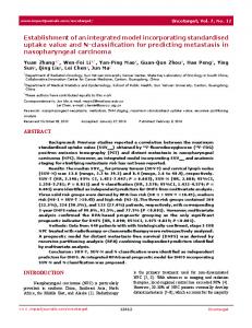
environment characterized in Figure 1, the system encodes a representation of every task cue in episodic memory and uses this representation to guide its behavior over subsequent trials, until the next cue is presented. We refer to this representation as a task code. We also assume that each task code lingers after its relevance expires, such that after N runs of trials, there will be N task codes in episodic memory. The significance of this is that on any given trial, when the system tries to retrieve the current task code, old ones could interfere. The core construct governing task-code processing in our model is activation. Every task code—and every other declarative memory element, as we note later— has an activation level, and when the system needs to retrieve a task code, memory returns the one with the highest activation at that instant. Given this constraint, the job of the cognitive system is to ensure that the current task code is more active than any other for the duration of the current run, and to encode a new task code when the next task cue is presented, such that the new one is the most active. The job is complicated by noise in activation levels, which can temporarily make an old task code more active than the current one, or which can temporarily push all task codes below threshold, thereby making the system transiently unable to remember what it is doing. These dynamics are adapted from the ACT–R cognitive theory (Anderson, 2007; Anderson et al., 2004; Anderson & Lebiere, 1998) but bear some similarity to other formal activation constructs (e.g., Hintzman, 1988; Just & Carpenter, 1992). Figure 2 shows a representation of these principles adapted from signal-detection theory. Each curve is a probability density function for the activation of a memory code: The abscissa represents activation level, increasing to the right, and the ordinate represents the probability of the code having a given activation level. The dispersion of the density function represents activation noise. Thus, when the system makes a retrieval request, the activation of a code is most likely to be at its mean level but may also be above or below, with decreasing probability the greater the distance from the mean. The bottom panel of Figure 2 shows density functions for the activation of two memory elements, which we interpret here as task codes in episodic memory (at other times, we interpret them as meaning codes in semantic memory, for which the activation dynamics are very similar). The density on the right is for the current task code, which is the retrieval target when the system needs to recall what task to perform on the current trial. The density on the left is for an old task code, which is a source of proactive interference. (In general, there are many old task codes in episodic memory, but there is no loss of generality in considering this simpler scenario for now.) The activation of the current task code is higher than that of the old task code (separation ⬎ 0), allowing the system to distinguish them; if this separation were zero, this would represent a situation of catastrophic interference in which the current task code would be indistinguishable from its predecessor. At the intersection of the two densities is the retrieval threshold, a high-pass filter that prevents the retrieval of codes whose activation is below threshold when the retrieval is attempted. The mean activation of the current task code is above threshold (gain ⬎ 0), and the mean activation of the old task code is below threshold (gain ⬍ 0); in general, gain can be high (far from threshold) or low (close to threshold). Gain affects accessibility, which is the area of a density function that lies above (to the

COGNITIVE CONTROL MODEL

605

Figure 2. Abstract representation of the cognitive control model, showing probability density functions for activation of memory elements. Top and middle: A task code is encoded in episodic memory, then decays during use. Bottom: The next task code is encoded and can govern performance because it is more active than the old one (separation ⬎ 0) and is above threshold (gain ⬎ 0). The bottom panel also applies to semantic memory; for example, the meaning of a presented task cue is perceptually primed and therefore more accessible (right-hand density) than the meaning of the not-presented cue (left-hand density).

right of) threshold; accessibility equals the probability that that memory element will be above threshold at a given instant. The top and middle panels of Figure 2 show supporting processes that allow the system to sustain the functional situation in the bottom panel—the current task code having positive gain and being more accessible than the old code—indefinitely across any number of task cues presented by the environment. The top panel shows encoding in response to the presentation of a task cue. Encoding, here, simply means creating a new task code and then raising its activation from some initial level (at the tail of the arrow) to a level at which the new code is accessible enough to meet performance requirements. The middle panel of Figure 2 shows the current task code decaying, or losing activation. Decay plays a functional role in our model, as an automatic architectural process that works in the background to prevent a catastrophic buildup of proactive interference. To appreciate the functional role of decay, consider what would happen if it were absent. The system could perhaps respond by encoding each new task code with a higher activation level than the previous one (to make the separation quantity in Figure 2 positive); however, assuming some biological or other upper bound on activation levels, this would make shifts of cognitive

control increasingly difficult and ultimately impossible. With decay, in contrast, flexible cognitive control is sustainable as long as each new task cue presented by the environment is encoded to an initial activation level that makes it more accessible than any old (decayed) task code in memory. Relative to inhibitory processing (e.g., Engle, Conway, Tuholski, & Shisler, 1995; Hasher & Zacks, 1988), decay can be viewed as similar in effect but more gradual and, critically, obligatory rather than controlled. An obligatory forgetting process would seem to be a useful and even necessary component of a cognitive system that must be able to update its declarative control representations frequently and continually over extended periods of performance. Moreover, in forcing the system to encode new control information periodically, decay would seem to help address what Newell (1990) construed as the “sudden death” problem of rogue control information hijacking behavior. For example, if the system happened to be struck by the impulse to jump in front of a bus, it would benefit if an automatic process forced it to reconsider, particularly if inhibition failed to deploy or was difficult to sustain for some reason. Thus, for a noisy system in a dynamic environment, a process that automatically triggers refresh of control representations seems to complement effortful inhibitory processing in important functional ways.

ALTMANN AND GRAY

606 Basic Phenomena

Here we link six basic behavioral effects to the abstract model described above. To illustrate each, we refer forward to Figures 7–11, which show the data from the experiment presented in Simulation Study 1. The phenomena are summarized in Table 1, which also serves as an index to the relevant figures and analysis tables. The six basic effects fall into two classes. In the first class are effects related to the encoding process in the top panel of Figure 2. There are two such first-trial effects, each measured on the trial in serial Position 1 of a run of trials, which immediately follows presentation of the task cue for that run, making it a locus of residual effects of the encoding process. The preparation effect (see Figure 7) is the change in Position 1 response latency as a function of the CSI between onset of the task cue and onset of the Position 1 stimulus; generally, the longer the CSI, the faster the Position 1 response latency, as cue-related processes have more time to complete their work before stimulus onset. Latency switch cost is the small (45 ms; see Figure 7) difference in Position 1 response latencies as a function of whether the just-presented task cue was a switch cue, signifying a different task than was performed on the previous run, or a repeat cue, signifying the same task as was performed on the previous run. We refer to this as “latency switch cost” to emphasize that latency and error switch costs in CCM arise from different underlying mechanisms. The second class consists of four within-run effects related to the decay process in the middle panel of Figure 2. Within-run slowing (see Figure 8) is a gradual increase in latencies across trials starting with Position 2, an effect we attribute to decay of the current task code. Within-run error increase (see Figure 9) is a corresponding trend in error rates, which is often noisier but is crucial to the interpretation of within-run slowing because it rules out a speed–accuracy tradeoff account of the two effects together.

A runlength effect that we have partially documented before (Altmann & Gray, 2002) is the finding that the slopes of within-run slowing and error increase vary inversely with the average number of trials between task cues—that is, the shorter the average runlength in a condition, the steeper the slope (see Figures 8 and 9). We describe this effect and develop a new runlength prediction in the next subsection. Finally, full-run error-switch cost, as distinct from the latency switch cost we noted above, is evident on all trials of a run, rather than just Position 1, and manifests in terms of errors (see Figure 10) but not response latencies (see Figure 11). In our model, this effect is caused primarily by memory errors in which old task codes intrude on the current task code, which are more likely to cause performance errors on switch runs than on repeat runs. We touch on these effects again in describing the computational implementation of CCM and describe them in more detail in Simulation Study 1, which is the context for the figures to which we have been referring. Table 1 also identifies two “other effects” that CCM reproduces and that we describe later but that do not directly flow from the abstract model.

Extending CCM: A Second Runlength Effect A prediction of the model in Figure 2 concerns the effect of varying the activation of the most active old code, which generalizes the left-hand density function in Figure 2 (bottom panel). Earlier we took this density to represent one old task code, but in the general case, it represents the activation of the most active of all old codes. If the system tries to retrieve the current task code and retrieves an incorrect task code instead, the intruder will have been the most active old code. The activation of the most active old code is the interference level (Altmann & Trafton, 2002).

Table 1 Summary of Behavioral Effects Reproduced by the Computational Implementation of the Cognitive Control Model Effects First-trial effects Preparation effect Latency switch cost Within-run effects Within-run slowing Within-run error increase Runlength effects Full-run error switch cost Other effects Congruency Failure-to-engage effects

Descriptions

Relevant figures

Relevant tables and contrasts

Position 1 latency faster with longer cue-stimulus interval Position 1 latency faster on repeat runs than switch runs

7

B1: Cue-stimulus interval

7

B1: Switching

Latencies increase gradually across positions within a run, starting with Position 2 Errors increase gradually across positions within a run, starting with Position 1 Effect of average runlength on slopes of withinrun slowing and error increase; main effect of average runlength on errors Main effect of switching on errors, driven by incongruent trials, on all positions in a run

8

B2: Position, main effects and linear trends

9

B3: Position, main effects and linear trends

8 9

B2: R ⫻ P B3: R ⫻ P, Runlength

10

B3: Switching, S ⫻ G

10 13 13 19

B3: Congruency B1: Congruency B2: Congruency

Fewer errors and faster latencies when the stimulus has the same response under both tasks Position 1 latency distributions shift and change shape with cue-stimulus interval

Note. R ⫽ runlength; P ⫽ position; S ⫽ switching; G ⫽ congruency.

COGNITIVE CONTROL MODEL

607

Figure 3. Effects of manipulating average runlength, expressed in terms of the constructs from Figure 2. The right-hand density function in each panel represents the activation of the current task code, and the left-hand density function in each panel represents the interference level, which is the activation of the most active old code. The interference level varies with the recency and number of old task codes. We assume that the system adjusts the retrieval threshold to adapt to the interference level.

Figure 3 shows how the interference level should be affected by varying the condition runlength—that is, the average runlength within a condition when the runlength in that condition is a random variable. The interference level is higher with a shorter condition runlength than with a longer condition runlength (compare the top and bottom panels of Figure 3). This is for two reasons. First, when the condition runlength is shorter, the most active old code is, on average, more recent and thus less decayed. Second, if a given number of trials per session are grouped into shorter runs (e.g., 100 runs of 10 trials/run) instead of longer runs (e.g., 50 runs of 20 trials/run), there are more runs and, thus, more old task codes in episodic memory. The larger the set of items in memory, the more active the most active of these tends to be (see, e.g., Anderson & Lebiere, 1998, Chapter 3, Appendix). Two predictions follow from this analysis. The first, which we noted in the previous subsection, is that the slopes of within-run slowing and error increase should be steeper in a short-runs condition than in a long-runs condition (as in Figures 8 and 9). The logic is illustrated by visualizing the two right-hand density functions in Figure 3—the one in the top panel and the one in the bottom panel— each shifting leftward by the same distance, reflecting a given amount of decay. This leftward shift decreases the accessibility of the current task code—the probability of it being above threshold— by a larger amount in the top panel than in the bottom panel, because in the top panel, a larger area of the density moves past the threshold during the shift. Thus, the change in accessibility of the current task code per unit decay is greater in a short-runs condition than in a long-runs condition, predicting steeper slopes for within-run slowing and within-run error increase in the short-runs condition. The second prediction, which is new here, is that the condition runlength should have a main effect on the frequency of performance errors, with these being more frequent in the short-runs condition than

in the long-runs condition. In Figure 3, within each panel, the retrieval threshold lies at the intersection of the two density functions, which in signal detection terms is the optimal location. We assume that the system adjusts the retrieval threshold to this location during initial performance at a given condition runlength. Under this assumption, the most active old code is more accessible in the short-runs condition (see the top panel of Figure 3) than in the long-runs condition (see the bottom panel of Figure 3), and the current task code is less accessible in the short-runs condition than in the long-runs condition. Thus, when a task code is retrieved, the probability that it is the most active old code is higher in the short-runs condition, causing more frequent performance errors.

A Computational Model In this section, we describe a computational implementation of the principles of operation described above. The purpose of the computational model is to demonstrate the sufficiency of these principles to exercise cognitive control in a situation in which proactive interference from old task codes is a real constraint and to do so in a way that reproduces a broad range of empirical phenomena. CCM is implemented in Version 4.0 of the ACT–R cognitive simulator (Anderson & Lebiere, 1998).2 We divide our description into five subsections. First, we describe the computational model’s memory organization and core mechanisms. Second, we describe how the model encodes a task code and relate this to first-trial effects. Third, we describe pro2 Model code, Excel spreadsheets for all figures and tables, and participant-level data for Simulation Study 1 are available at www .msu.edu/⬃ema/taskswitching.

608

ALTMANN AND GRAY

cessing stages common to all trials, including a task-code retrieval stage, called task focusing, that we relate to within-run effects. Fourth, we step through a performance trace spanning cue encoding and a couple of trials, to illustrate the various processes we have described by that point. Fifth and finally, we describe the model’s activation-related parameters and how we adjusted them to fit the model to empirical data.

Declarative Memory Organization and Core Mechanisms CCM’s declarative memory organization is shown in Figure 4. There are episodic elements (the four at the bottom) and semantic elements (shown in the middle). Percepts (shown at the top) are symbols represented within the system when a task cue or trial stimulus is presented, which then have to be identified by retrieval of their meaning. The arrows connecting elements of Figure 4 represent associative links that spread activation between elements. At runtime, several of these elements at various times are retrieved to the system’s focus of attention, from whence they spread activation to their associates. The focus of attention is a limited-capacity immediate memory that can be accessed without time cost or error, and is the source of spreading activation, which we refer to simply

as priming. The total amount of priming is fixed and is divided equally among the elements in focus (primes), each of which spreads its share to every memory element to which it is directly linked (Anderson, 2007; Anderson et al., 2004; Anderson & Lebiere, 1998). One important kind of priming, for example, is perceptual: When a task cue onsets, CCM’s (grossly simplified) perceptual system installs a cue percept in the focus of attention, and this percept then primes its meaning in semantic memory. All the associative links in Figure 4 influence some aspect of CCM’s behavior and are discussed later in a relevant context. Any priming reaching a given element (semantic or episodic) is added to that element’s base-level activation to determine the element’s total activation. Semantic memory elements have a stable base-level activation over the lifetime of the model, which is one experimental session. Episodic memory elements, which are all task codes, have a base-level activation that changes with time. A task code’s activation increases during encoding, from zero to a peak value that is a model parameter. The code then loses activation (decays) per the function Base-level activation of task code ⫽ ln (2 ⫻ encoding-cycles/T0.5),

Figure 4. Declarative memory organization in the computational implementation of the cognitive control model. Priming spreads through an associative link from the element at the tail of the link to the element at the head of the link when the tail element enters the focus of attention to become a prime.

(1)

COGNITIVE CONTROL MODEL

in which encoding-cycles is the parameter that governs the peak value of task-code activation, and T is the time since encoding finished. Equation 1 produces negatively accelerating decay, a pattern we examine at the end of Simulation Study 1. Activation noise, represented by the dispersion of the densities in Figures 2 and 3, is sampled from a zero-mean logistic density function independently for every memory element on every system cycle and is added to that item’s total activation for that cycle. This noise mechanism has an important implication: If a memory retrieval fails on one system cycle, because all elements happen to fall below threshold at that instant, another attempt on the next system cycle may succeed. This, in turn, means that the system can trade speed against accuracy in memory retrieval. For example, if the system sets a high threshold, this reduces the probability of a retrieval error, meaning an intrusion by some distracting element whose activation is transiently highest at that moment. However, a high threshold also increases the probability of a retrieval failure, meaning a situation in which no element is above threshold on that cycle. A retrieval failure wastes that system cycle, but the system can try again on the next cycle. Thus, by setting a higher retrieval threshold, the system can make retrieval more accurate, at the cost

609

of more retrieval failures and, thus, longer average retrieval latencies. Retrievals are directed by productions, which are fine-grained units of control knowledge (see Figure 5) that use the information they retrieve to do some work, like altering the contents of the mental focus of attention. On a given system cycle, one production is selected from the conflict set, which is the set of all productions that match the current contents of the focus of attention (see also Anderson & Lebiere, 1998). The production selected from the conflict set is the one with the highest value, just as the element retrieved from declarative memory is the one with the highest activation. Production values, like activation values, are subject to transient noise sampled independently for each production on each system cycle, which means that the production selected from the conflict set can vary across cycles, even if the conflict set is the same. When a production is selected, it can request that an element be retrieved from declarative memory, such as a task code, or a cue meaning; the system then finds the most active element of that type. If that element is above threshold, it is retrieved, and the production fires, doing some work. If a retrieval request fails, that system cycle is wasted, and the system selects from the conflict set

Figure 5. The productions in the computational implementation of the cognitive control model, in pseudocode. On all system cycles, the conflict set contains two productions, one of them task-related, the other the unrelated-process production, which wastes a cycle if selected.

610

ALTMANN AND GRAY

again on the next cycle. Figure 5 summarizes, for each of CCM’s productions, the conditions under which that production is selected, any retrieval it might direct, and the action it takes. We discuss conflict resolution in more detail in Appendix A. The duration of a system cycle is 50 ms, on average, regardless of whether the selected production fires or not. The actual duration of a given cycle is sampled from an exponential density with a mean of 50 ms independently on every cycle.

Encoding a Task Code When the environment presents a task cue, this triggers an encoding process that creates and activates a new task code in episodic memory to govern performance for the subsequent run of trials. In terms of Figure 2 (top panel), encoding is represented by the density function for a newly created task code shifting right along the activation axis toward its end location (decay in reverse, and faster). Encoding starts sometime after cue onset and may not finish until after the stimulus has onset for the Position 1 trial, which means that encoding contributes to average Position 1 response latency. Encoding starts with the identify-cue production (see Figure 5). Identify-cue is in the conflict set whenever a cue percept is in the focus of attention but there is no cue meaning in focus yet. If identify-cue is selected on a given cycle, it tries to retrieve a cue meaning from semantic memory. If activation noise has pushed all cue meanings below threshold at that instant, the retrieval fails, and that cycle is wasted. If the most active meaning is above threshold, it is retrieved, and identify-cue fires, creating a new task code with that meaning and with an initial activation value of zero. Identify-cue is the locus of latency switch cost (see Table 1). A repeat cue’s meaning is repetition primed and therefore more accessible than a switch cue’s meaning, so identify-cue fires sooner, on average, when a repeat cue is presented, causing encoding to start sooner and thus end sooner. After identify-cue fires, encoding continues with the activate-tc production (see Figure 5). This fires repeatedly, with each firing incrementing the task code’s activation (see Just & Carpenter, 1992, for a similar mechanism in which productions “pump” activation into memory elements). The number of firings, and thus a task code’s peak activation level, is governed by the value of the encoding-cycles parameter in Equation 1. The encoding process as a whole is the locus of the preparation effect (see Table 1), in which a longer CSI leads to faster latency (on the cued trial). In CCM, the preparation effect is caused by a larger proportion of total encoding cycles falling into a longer CSI than into a shorter CSI. Empirically, the relationship between CSI and response latency is usually not one-to-one, however, in that a given increase in CSI is not fully matched by the corresponding decrease in response latency. We explain this undermatching in terms of a higher efficiency of encoding at shorter CSIs, such that the system makes better use of available encoding time when there is less time available. More formally, encoding efficiency is the probability that the value of the relevant encoding production (identify-cue if it has not already fired, active-tc if it has) is higher than the mean value of productions unrelated to task switching. These unrelated productions are represented in terms of one generic unrelated-process production (see Figure 5). Production values are noisy, like activation values (see Figure 2), so the

unrelated-process production can be selected over an encoding production if its value is transiently higher. The function relating encoding efficiency to CSI is Encoding efficiency ⫽ 1 ⫺ ␦ ⫻ (CSI/100),

(2)

meaning simply that efficiency is higher at smaller CSI, measured here in milliseconds. The parameter ␦ is the rate of change of encoding efficiency with CSI; this is a free parameter that we estimated to fit the preparation effect in Simulation Study 1 and then held constant in Simulation Studies 2 and 3. We discuss encoding efficiency in more detail in Appendix A. This assumption of greater encoding efficiency at short CSIs seems to have some face validity. Its functional relevance could lie in reducing the number of “missed” cues at short CSIs, while at the same time making more system cycles available to other processes during the CSI at long CSIs. Such a mechanism would seem to be qualitatively consistent with foreperiod effects (e.g., Luce, 1986; Posner & Boies, 1971), if the value of encoding productions is taken to represent preparedness, which is aversive to maintain over time. However, these are speculations, and we have not yet modeled how the system actually benefits from adapting to cue duration, nor have we asked how the system might adjust the relevant production values (e.g., Anderson, 2007; Fu & Anderson, 2006). We adopted the efficiency formalism in Equation 2 because it is simple, does well at capturing the variance in our data (see Figure 7), and does so with only one free parameter (␦) that has to be estimated through model fitting.

Trial Processing When the environment presents a stimulus—the digit 8, for example—this triggers trial processing, which consists of three serial stages. The first stage, task focusing, involves adding a task to the focus of attention by retrieving a task code from episodic memory. (Task focusing seems to map quite directly to the taskdecision process of Meiran & Daichman, 2005.) The second stage involves using the task code to identify the stimulus along the relevant dimension. The third stage involves using the stimulus category to select a response. Below we describe each stage in more detail, identifying in particular how task focusing leads to within-run effects (see Table 1). Task focusing is carried out by the retrieve-tc production (see Figure 5), which is in the conflict set when a stimulus percept is in the focus of attention but there is no task in focus to help interpret it. When retrieve-tc is selected, it tries to retrieve a task code. If no task code is above threshold, the retrieval fails, that system cycle is wasted, and the system has to try again. As the current task code decays, such retrieval failures become more frequent, causing within-run slowing. When a task code is finally retrieved, retrieve-tc adds the task it codes to the focus of attention. The retrieved code will usually be the current one, but a task-focusing error may also occur, meaning that the retrieved code is from a previous run or from even older, unrelated performance (examples of current, old, and unrelated-task codes appear in the bottom panel of Figure 4). If the intruding code is from a previous run, the system goes on to perform that task on the current trial—leading to full-run error switch cost, because the intruding code represents the wrong task more often on switch runs than on repeat runs. If the intruding code is from even older, unrelated performance, the

COGNITIVE CONTROL MODEL

system treats it as uninterpretable and simply guesses a response, bypassing the remaining stages of trial processing (described next). Both kinds of intrusion contribute to within-run error increase, because they become more frequent as the current task code decays relative to old task codes. After task focusing, the identify-stimulus production (see Figure 5) tries to retrieve a category for the stimulus. Each stimulus is associated with two categories, one for each task, and priming from the task in focus gives the advantage to the correct one. For example, per Figure 4, the stimulus “7” primes “high” and “odd,” and the task “evenodd” primes categories “even” and “odd,” making “odd” the only category primed by two sources and, thus, the most active. After the stimulus is identified, the select-response production tries to retrieve a response from semantic memory. Responses are primed by the appropriate stimulus category; per Figure 4, if the category “odd” is in focus, it primes retrieval of the

611

“right” response. After the response is selected, it is executed. The time needed for the execute-response production to fire is a parameter that we use to adjust response latency uniformly over positions, to account for motor and other processes whose operations may take more than one production’s worth of work; all other productions fire in 50 ms, but execute-response takes 345 ms, as estimated in Simulation Study 1. Response execution clears the task from the focus of attention, such that task focusing occurs again on the next trial; the theoretical interpretation is that immediate memory for control information has a very short duration.

A Process Trace Figure 6 shows a process trace spanning cue encoding and two trials. We step through the trace here to tie together the mechanisms we discussed above and to comment on an important as-

Figure 6. A cycle-level trace of the computational implementation of the cognitive control model, spanning the identification of a task cue (Cycle 1), the encoding a new task code in episodic memory (Cycles 2–15), and performance of the first two trials of the following run (Cycles 16 –24). See Figure 5 for production pseudo-code.

ALTMANN AND GRAY

612

sumption about modularity of encoding and retrieval. The left column of Figure 6 locates the onset of percepts—a task cue and three trial stimuli—and the right column identifies the production selected on each cycle. The task cue “Even Odd” onsets first, after which CCM selects the identify-cue production on Cycle 1; this fires, meaning that the system was able to retrieve a cue meaning from semantic memory and use this information to create a new task code. Encoding continues with activate-tc, which is selected and fires on Cycle 2 and again on Cycle 3. On Cycle 4, CCM’s attention lapses, as it were, with noise in production values causing the unrelatedprocess production to be selected. At this point, the task cue offsets and the Position 1 stimulus (“8”) onsets. Encoding is not complete, however, so activate-tc is selected again on Cycle 5. For the next several cycles (marked in Figure 6 by an ellipsis), CCM continues to select activate-tc and occasionally unrelated-process. Cycle 15 marks the end of encoding, with activate-tc firing for the 10th time, reflecting the value of 10 for the encoding-cycles parameter (see Equation 1) in Simulation Study 1. Trial processing begins on Cycle 16, with retrieve-tc being selected. Here we note an important assumption, which is that task focusing is necessary even when it is preceded immediately by encoding. In other words, the two processes are modular, in the sense that encoding cannot substitute for retrieval. This assumption drives our account of explicit-cuing performance in Simulation Study 2, where we argue that explicit-cuing response latencies accommodate both processes on every trial, including cued trials. Retrieve-tc fires, which it usually does when selected so soon after task encoding, given that the new task code is at its peak

activation and highly accessible. The task code delivered by the memory system was “evenodd 42,” designated as such to signify that it was encoded from the 42nd task cue presented in this hypothetical session. CCM then identifies the stimulus as “even” (Cycle 17), retrieves the response category “left” (Cycle 18), and executes the response (Cycle 19), triggering onset of the Position 2 stimulus (“7”). Retrieve-tc is selected to start the next trial (Cycle 20), but no task code is above threshold (the current code is now slightly decayed, and activation is noisy), so the retrieval fails; retrieve-tc is then selected again (Cycle 21), and this time the retrieval succeeds. Trial processing then continues as before, leading to onset of the Position 3 stimulus (“4”).

Priming and Other Activation-Related Parameters Here we describe the parameters governing CCM’s activation dynamics, focusing on how they affect retrieval from semantic memory. Parameter names and values appear in Table 2. The upper section of the table shows parameters for the retrieval threshold, the base activation levels of different memory codes, and the standard deviation of activation noise. The lower section of the table shows parameters that affect how much priming flows through the various links in declarative memory (see Figure 4). Perceptual priming flows from a cue percept (e.g., “Even Odd” in Figure 4) to its meaning in semantic memory (“evenodd”), semantic priming flows from one element of semantic memory to another (e.g., from “evenodd” to “even” and “odd”), and repetition priming flows from the current task code to its meaning and to itself. In all these forms of priming, an element

Table 2 Parameters Governing Activation in the Computational Implementation of the Cognitive Control Model Parameter

Units of activation

Retrieval threshold . . . in long-runs condition of Simulation Study 1 Peak base-level activation of task codes Semantic base-level activation Activation of unrelated-task code Activation noise standard deviation Prime Perceptual prime Cue (Even Odd) Stimulus (8) Congruent stimulus (8) Semantic prime Task (evenodd) Category (even) Repetition prime Current task code Current task code

7.02 6.78 4.94 2.47 3.77 1.30 Target

Share

Weight

Units of activation

Its meaning (evenodd) Before stimulus onset After stimulus onset Its categories (even, high) Its response (left)

0.35 0.33 0.33 0.33

13.0 13.0 13.0 13.0

4.55 4.33 4.33 4.33

Its categories (even, odd) Its response (left)

0.33 0.33

16.5 16.5

5.50 5.50

Its meaning (evenodd) Before stimulus onset After stimulus onset Itself

0.35 0.33 0.50

3.4 3.4 8.7

1.19 1.13 4.35

Note. Values in bold were estimated to fit the data in Simulation Study 1, values in roman font are yoked to bold values, and values in italics are fixed by representational constraints. Share is the proportion of the source amount of priming allocated to that prime, and weight multiplies share to determine the amount of priming reaching the target. The value of 4.94 for peak base-level activation of task codes corresponds to a value of 10 for the encoding-cycles parameter in Equation 1: Base-level activation of task code ⫽ ln(2 ⫻ encoding-cycles/T0.5). Two parameters, encoding-cycles and cue-priming weight, changed in Simulation Studies 2 and 3.

COGNITIVE CONTROL MODEL

becomes a prime at runtime when it enters the focus of attention, by action either of the perceptual system or of some production firing. A constraint on priming that we noted earlier is that there is a fixed source amount divided equally among the primes in the focus of attention, meaning that the more primes are in focus, the less activation is available to each to spread to its targets. Each prime’s share of the source amount is multiplied by the weight of the link between it and its target(s) to determine the amount of priming that spreads to its target(s). For example, when a cue percept is added to the focus, its share of the source amount is 0.35 (see Table 2). This share is multiplied by a weight of 13.0, priming the cue’s meaning with 4.55 units of activation. These are added to the 2.47 units of base-level activation, bringing the meaning’s mean activation to 7.02 units, or roughly to threshold. Thus, with respect to Figure 2 (bottom panel), the cue meaning’s accessibility is about 0.5 during the CSI; that is, when identify-cue is selected, it has a 50% chance of firing. When a stimulus then onsets to start the Position 1 trial, the cue’s share of the source amount drops to 0.33.3 Thus, the stimulus percept siphons some of the source amount away from the cue percept, making the cue meaning slightly less accessible, a point that becomes relevant in Simulation Study 2 in our account of the CSI ⫻ Switching interaction. If a prime is linked to multiple targets, it primes all of them. For example, a stimulus percept (e.g., “8” in Figure 4) is linked to two categories (“even” and “high”), and when it is added to the focus, it primes both (in each case, by its full share times the weight). Each category’s gain increases equally as a result, which means that additional priming from the task meaning in focus (e.g., “evenodd”) is needed to increase the gain further for the correct category (“even”) and ultimately produce a correct response. The parameters we adjusted to fit the data in Simulation Study 1 are shown in bold in Table 2. The retrieval threshold took two values, per the analysis surrounding Figure 3; Simulation Studies 2 and 3 used the short-runs value. Two other parameters—the weight on perceptual priming, and the value of encoding-cycles, expressed in Table 2 as peak base-level activation of a task code—took different values in Simulation Studies 2 and 3, as we discuss in context there. Apart from these changes, all other parameter values were held constant within and between simulations. Appendix A describes the parameters and their interactions and constraints in more detail. To fit CCM to empirical data, we estimated the bold parameter values in Table 2 to try to minimize root-mean-squared deviation between the aggregate empirical data and aggregate simulated data (aggregated over simulated participants). Because the model generates its own variability and because each simulated experiment is time-consuming (taking about 45 min on a 3-GHz Intel processor), this minimization could only be approximate. Root-mean-squared deviation and proportion of variance accounted for (r2) appear in the caption of each figure that compares empirical and simulated data.

Simulation Study 1: Randomized Runs Here we show that CCM can simulate the phenomena summarized in Table 1 by fitting it to new data collected using the randomized-runs procedure. The most relevant independent variables in the new experiment are CSI (with eight levels varied between participants), the average runlength in a condition (two levels, also varied between participants), switching (switch runs,

613

repeat runs), and trial position within a run (for those positions common to both condition runlengths). The full method for the experiment and analysis of variance tables for the results are given in Appendix B. We describe the empirical and simulated data below, in six subsections, corresponding to the six core phenomena outlined in Table 1. In the Discussion, we present two further analyses of CCM’s performance, one tracing activation levels sampled from the running model, and one showing how CCM accommodates effects of stimulus–response congruency on response latency.

The Preparation Effect This effect, shown in Figure 7, is the decrease of Position 1 latency with increase in CSI. In CCM, encoding productions have to fire some number of times, once to retrieve the cue’s meaning and then several times to activate the new task code. These firings can occur anytime after cue onset, but there is no deadline for when they must complete, and selection from the conflict set is affected by noise in production values sampled independently between cycles. Thus, encoding can spill over past onset of the Position 1 stimulus (Altmann, 2002), adding to Position 1 latency. Fewer such firings spill over after a longer CSI, causing the preparation effect. The range of change of CSI is larger than the range of change in Position 1 latency, a pattern CCM reproduces through Equation 2, which links encoding efficiency to CSI. Equation 2 produces a weakly negatively accelerating trend in CSI, and although the empirical data show a similar trend, only the linear contrast was reliable (see Table B1).

Latency Switch Cost This effect, also shown in Figure 7, is the difference between Position 1 switch latencies and Position 1 repeat latencies. In CCM, the task code from the preceding run is still in the focus of attention as the current task code is being identified, and repetition priming flows from the old code to its meaning. (In Figure 4, a representative link is from “evenodd 42” to “evenodd.”) This makes the meaning more accessible, which facilitates retrieval of the meaning by the identify-cue production in the repeat case, which in turn allows identify-cue to fire sooner after cue onset in 3 This share of 0.33 and the share of 0.35 noted earlier were computed as follows. The default value for the source amount in ACT–R is 1.0 (reflecting its role as a multiplier), so if there are p primes in focus, each gets 1/p of the source amount. After stimulus onset on the Position 1 trial, the focus of attention contains three elements: the percept for the cue that was just presented (which remains in focus through encoding); the percept for the Position 1 stimulus; and a task code, either the current one, if identify-cue (see Figure 5) has already fired, or the one from the previous run, if identify-cue has not yet fired. With three primes in focus, the cue percept’s share of the source amount is 0.33. However, before stimulus onset, when there were only two primes in focus (the cue percept and a task code), the cue percept’s share was 0.35 (see Table 2), not 0.50. This is because we use the value of the source amount before stimulus onset as the parameter that governs the magnitude of the effect of stimulus onset on cue priming. Thus, before stimulus onset, the source amount is 0.7 (an estimated value), and after stimulus onset, this reverts to 1.0. For simplicity, in Table 2, we identify this parameter with the value of 0.35 (shown in bold).

ALTMANN AND GRAY

614

Figure 7. Empirical and simulated response latencies from Simulation Study 1, for the Position 1 trial, separated by cue-stimulus interval and switching. Effects shown are the preparation effect and latency switch cost (see Table 1). Root-mean-squared deviation ⫽ 39.7 ms, r2 ⫽ .87.

the repeat case. (Repetition priming also affects encoding of switch cues, increasing the frequency of encoding errors; this mechanism is described in Appendix A.) The CSI ⫻ Switching interaction was null in the empirical data, meaning that latency switch cost was unaffected by CSI. In CCM,the interaction was null because two processes worked against each other; we develop our account of these processes in detail in Simulation Study 2, where we offer an explanation of why the interaction seems to depend on situational factors, such as how CSI is manipulated (between or within participants).

2). In CCM, within-run error increase, like within-run slowing, stems from decay of the current task code. In terms of Figure 2, decay causes the accessibility of the current task code to decrease relative to the accessibility of the most active old code, which increases the probability of a task-focusing error. CCM reproduces the empirical dissociation between latencies and errors on Position 1 (compare Figures 8 and 9). Simulated latencies are elevated on Position 1 because they reflect encoding, which is limited to Position 1. Simulated errors are not elevated on Position 1, because they originate in processing common to all trials.

Within-Run Slowing This effect, shown in Figure 8, is the gradual increase in response latencies across positions, starting with Position 2. In CCM, within-run slowing stems from decay of the current task code. In terms of Figure 2 (middle panel), the density function for the current task code shifts gradually leftward, reducing accessibility of this code and increasing the probability that the retrieve-tc production will fail to fire when it is selected, such that the system has to try again. Within-run slowing in the long-runs condition also shows a higher-order trend, visible in the lower panels of Figure 8. This trend seems to be a consequence of curvilinear decay interacting with the shape of the activation density function, as we suggest in the Discussion, and possibly of a nonlinear relationship between accessibility and retrieval time that we address in more detail in Simulation Study 2. Empirically, the contrast for the cubic trend in position was reliable (see Table B2). Although empirical evidence for within-run slowing is evident in a number of studies (Monsell, Sumner, & Waters, 2003; Pashler, 1994; Poljac, de Haan, & van Galen, 2006; Poljac, Koch, & Bekkering, in press; Waszak, Hommel, & Allport, 2003), our account of the effect, here and in previous work (Altmann, 2002, 2004a; Altmann & Gray, 2002) is so far the only one that has emerged.

Runlength Effects

Within-Run Error Increase

Full-Run Error Switch Cost

This effect, shown in Figure 9, is the gradual increase in error rates across positions in a run, starting with Position 1 (not Position

This effect, shown in Figure 10, is the difference in error rates between incongruent switch trials and incongruent repeat trials,

One runlength effect is that the slopes of within-run slowing (see Figure 8) and within-run error increase (see Figure 9) are steeper in the short-runs condition than in the long-runs condition. In CCM, when the retrieval threshold is higher to compensate for a higher interference level (see Figure 3, upper panel), a given unit of decay produces a larger change in accessibility and, thus, greater rates of change within a run. The other runlength effect is that errors overall are more frequent in the short-runs condition. In CCM, this effect is due to the higher interference level in the short-runs condition. It is important to note that the runlength effect on slopes of within-run slowing and error increase seems to rule out an account of these effects in terms of retroactive interference, which could be a factor if each additional trial in the current run helps to bury the current task code a little deeper in episodic clutter (e.g., Wixted, 2005). A retroactive interference account would link the slope of within-run slowing and error increase to position alone. However, position interacted with condition runlength, for both latencies (see Table B2) and errors (see Table B3). Thus, even if retroactive interference does contribute to within-run effects, it cannot be the only factor.

COGNITIVE CONTROL MODEL

615

Figure 8. Empirical and simulated response latencies from Simulation Study 1. Effects shown are within-run slowing and the runlength effect on the slope of within-run slowing (see Table 1). Top panels: Positions 1– 8 (short runs) and 1–14 (long runs); root-mean-squared deviation (RMSD) ⫽ 7.5 ms, r2 ⫽ 1.00. Bottom panels: Positions 2– 8 (short runs) and 2–14 (long runs) on a magnified scale; RMSD ⫽ 4.1 ms, r2 ⫽ .98.

across the full run of trials. Incongruent trials are those on which the correct response to the stimulus differs depending on the task. (In Figure 4, “7” is an incongruent stimulus, whereas “8” is congruent; we return to congruency effects again in the Discussion.) In CCM, task-focusing errors cause performance errors more often on switch runs than on repeat runs, because the most

active old code is more likely to represent the wrong task on switch runs than on repeat runs, and this constraint only affects accuracy on incongruent trials (on which the correct response depends on the task). It is important to note that performance errors seem to have the same empirical signature in the explicit-cuing procedure, in

Figure 9. Empirical and simulated error percentages from Simulation Study 1, for Positions 1– 8 (short runs) and 1–14 (long runs). Effects shown are within-run error increase, the runlength effect on the slope of within-run error increase, and the main effect of runlength on errors (see Table 1). Root-mean-squared deviation ⫽ 0.27%, r2 ⫽ .82.

616

ALTMANN AND GRAY

Figure 10. Empirical and simulated error percentages from Simulation Study 1, for Positions 1– 8 (short runs) and 1–14 (long runs), separated by switching and congruency (curves within panels). The effect shown is full-run error switch cost (see Table 1), which is a main effect of switching driven by a Switching ⫻ Congruency interaction (see Table B3). Root-mean-squared deviation ⫽ 0.51%, r2 ⫽ .90.

terms of switching and congruency contrasts (Meiran & Daichman, 2005; Steinhauser & Hubner, 2006). If performance errors in explicit cuing are in fact task-focusing errors, this would seem to mean that the memory-based control mechanisms we associate with randomized-runs performance also support explicit-cuing performance, a point to which we return in Simulation Study 2. For comparison with the error data in Figure 10, we plot response latencies in Figure 11 in the same format. Empirically, there is actually a small but reliable switch benefit of 3.0 ms on Positions 2– 8 (see Table B2). In CCM, this benefit is related to latency switch cost on Position 1. Encoding can end during the CSI, before onset of the Position 1 stimulus, and when it does, there is a brief interval for the current task code to decay before the run starts. On average, this interval is longer for repeat cues than for switch cues, because the identify-cue production fires sooner for repeat cues. Thus, on average, the current task code is slightly more decayed during a repeat run than during a switch run. In the simulated latencies, the resulting benefit is an even smaller 1.8 ms, which we know is systematic only because a similar benefit occurs consistently across replications of the simulated experiment (and because there is a cause). The prediction is that any factor that increases latency switch cost should also increase this small switch benefit on later trials, although the small effect size—␩2 ⫽ .036 for the main effect of switching in Table B2—suggests that this could be an expensive prediction to test.

Discussion In this article, we attempt four types of integration, and in this first study, we have demonstrated three. Every mechanism we have proposed to explain some effect in Table 1 has some functional reason to exist; encoding accounts for first-trial effects, for example, and decay accounts for within-run slowing and error increase, and both encoding and decay are necessary to sustain flexible control given continual buildup of interference. Effects that may seem unrelated, such as long Position 1 latencies and within-run slowing, are related by underlying mechanisms, in that without one (reflecting encoding), there would not be the other (reflecting decay). We have focused mainly on assembly of existing constructs, rather than fabrication of new ones, and the constructs themselves all relate to the same underlying activation dynamics (see Figure 2, bottom panel). In Simulation Studies 2 and 3, we show that the same principles of operation transfer to other experimental procedures with what seem to be different performance requirements. We close this study with two supporting analyses. First, we examine activation levels sampled directly from the running model, to illustrate the decay pattern that results from Equation 1. This analysis lays some groundwork for Simulation Study 2 and lets us illustrate a chain of constraints leading from decay through the empirical trajectory of within-run slowing to latency switch cost. Second, we show how the model can account for latency congruency effects, which are not central to cognitive control at

COGNITIVE CONTROL MODEL

617

Figure 11. Empirical and simulated response latencies from Simulation Study 1, for Positions 1– 8 (short runs) and 1–14 (long runs), separated by switching (curves within panels). Root-mean-squared deviation ⫽ 8.5 ms, r2 ⫽ .99.

the level we have emphasized, but which nonetheless offer a useful test of CCM’s generality. Activation within a run. Figure 12 shows the activation of the current task code and most active old code over a run of trials, for short and long runlength conditions. The two curves at the top show activation of the current task code (for each runlength). The two lines in the middle are the retrieval thresholds. The two curves at the bottom show activation of the most active old code. The information in Figure 12 overlaps with that in Figure 3; the activation levels in Figure 12, taken at some specific run position and rotated 90 degrees clockwise, correspond to the means of the densities in Figure 3. The decay produced by Equation 1 is curvilinear, with a sharp decrease initially after encoding that then tapers off. This pattern raises a question about how CCM reproduces the trajectories of within-run slowing and error increase, which are close to linear. The answer lies in the interaction of curvilinear decay with a bell-shaped density function for activation noise. The interaction can be visualized in the context of the lower panel of Figure 2. The density function for the current task code starts far to the right of threshold, then shifts to the left, rapidly at first (reflecting rapid initial decay), then more slowly. Initially, then, when accessibility is high and decay is rapid, the result is only a moderate decrease in accessibility per unit time. Later in a run, when accessibility is lower and decay is slower, the result is again only a moderate decrease in accessibility per unit time. Thus, two nonlinear functions (decay and activation noise) balance out to yield a relatively

even rate of change in accessibility and, thus, yield relatively linear trajectories for within-slowing and error increase, modulo the cubic trend in within-run slowing in the long-runs condition (see Figure 8, bottom panels, and Table B2). The decay rate of 0.5 in Equation 1 is usually treated as a fixed parameter in ACT–R (Anderson & Lebiere, 1998), thereby constraining the standard deviation of activation noise to be such that it yields this relatively constant change in accessibility per unit time. The logic above ultimately grounds latency switch cost in a functional mechanism—not task-set reconfiguration (Monsell, 2003), but repetition priming, which supports memory accuracy in the face of high activation noise. Repetition priming contributes to the vertical separation between the current and most active old codes in Figure 12, also represented as the horizontal distance between means in the bottom panel of Figure 2. Decay also contributes to this separation but not enough to keep task-focusing errors to a tolerable level, given the standard deviation of activation noise, which itself is constrained, per our logic above. Thus, a set of interrelated constraints—including a fixed curvilinear decay function, activation noise, and task focusing on the theoretical side, and a particular pattern of within-run slowing and a low error rate on the empirical side—implies a functional need for repetition priming, which then causes latency switch cost as a side effect. Although we are not the first to link repetition priming to latency switch cost (Altmann, 2002; Dreisbach, Haider, & Kluwe, 2002; Gilbert & Shallice, 2002; Koch & Allport, 2006; Logan & Bundesen, 2003; Meiran, Chorev, & Sapir, 2000; Sohn & Ander-

618

ALTMANN AND GRAY

Figure 12. Activation of the current task code and the most active old code across trials in the current run. Circles represent Simulation Study 1 (randomized-runs procedure), separated by condition runlength. X’s at Position 1 represent Simulation Study 2 (explicit-cuing procedure).

son, 2001; Yeung & Monsell, 2003), we do seem to be the first to argue that repetition priming nonetheless plays a functional role in cognitive control. This argument emerged from the simulation approach we took to understanding the cognitive mechanisms of interest; specifically, CCM is demonstrably unable to reproduce empirical levels of accuracy without repetition priming, once all other constraints are satisfied. Latency congruency. Here we address the latency congruency effect, one of the “other effects” listed in Table 1. The empirical finding is that congruent stimuli— ones for which the response is the same under either task— elicit faster responses than incongruent stimuli, for which the response is different depending on the task. The model’s core mechanisms do not predict this effect directly but do suggest a natural way to accommodate it, one that happens to accord with empirical results dissociating the latency effect from the corresponding error effect (Meiran & Kessler, 2008). Figure 13 shows empirical and simulated latency congruency effects. Empirically, the effect seems to be linked to trial processing, because it registers on all positions of the run. We linked the effect to response selection, which is one of the stages of trial processing. The select-response production tries to retrieve a response when there is a stimulus category in focus. The stimulus category primes this retrieval, and when the stimulus is congruent, the stimulus itself also primes this retrieval. (In Figure 4, the stimulus category “even” and

the stimulus “8” both prime “left.”) The underlying assumption, for which there is empirical support (Hubner & Druey, 2006; Kiesel, Wendt, & Peters, 2007), is that a separate associative link is formed between a congruent stimulus and its response. Thus, priming from a congruent stimulus reduces retrieval failures during response selection and, thus, retrieval time. It also reduces retrieval errors and, thereby, performance errors, but error congruency effects come primarily from task-focusing errors, as we discussed in context of full-run error switch cost.

Simulation Study 2: Explicit Cuing Here we generalize CCM to the most commonly used taskswitching procedure, explicit cuing, in which a randomly selected task cue appears before every trial. Procedurally, explicit cuing is a special case of randomized runs in which runlength is fixed at one, and this is also how we treat it theoretically, by using the same mechanisms to simulate performance here as in the randomizedruns context. We have three specific aims for this study: (a) to make a case that our account of Position 1 latencies generalizes to the explicitcuing context; (b) to show that CCM can reproduce accurate performance with very short runs (of length one), which allow very little time for old task codes to decay; and (c) to develop an

COGNITIVE CONTROL MODEL

619

Figure 13. Empirical and simulated response latencies from Simulation Study 1, for Positions 1– 8 (short runs) and 1–14 (long runs), separated by congruency (curves within panels). Root-mean-squared deviation ⫽ 8.9 ms, r2 ⫽ .99.

account of the CSI ⫻ Switching interaction that addresses why it seems to depend on how CSI is manipulated. The data we focus on here come from Koch (2001), the first study to report a null CSI ⫻ Switching interaction (see also Simulation Study 1, as well as Altmann, 2004a, 2004b, 2006; Poljac et al., 2006; Proctor, Koch, & Vu, 2006; Proctor, Koch, Vu, & Yamaguchi, in press; Steinhauser et al., 2007). Koch’s Experiments 1 and 3 were identical in method except that each used a different, constant value of CSI; he compared them statistically, with experiment as a factor to represent a between-participants manipulation of CSI, and found a null CSI ⫻ Switching interaction. He then blocked CSI within participants in his Experiment 4, and the interaction reappeared, a finding replicated by Altmann (2004b). We simulate both these data sets from Koch (2001), plus data from a design in which CSI was randomized within participants (Logan & Bundesen, 2003, Experiment 5).

Explicit-Cuing Latencies as Position 1 Latencies Here we ask whether explicit cuing latencies are similar in magnitude to Position 1 latencies in the randomized-runs procedure and whether they respond similarly to CSI manipulations. If it is so in both cases, this would point to similar underlying processes and, thus, on the basis of our account of first-trial effects in Simulation Study 1, to a role for task codes in episodic memory supporting performance, even when every trial is perceptually cued. Figure 14 shows response latencies from Koch’s (2001) CSIbetween analysis (left panels) and simulated data from CCM (right

panels). The simulated data in the upper right panel reflect just the relevant procedural changes to CCM relative to Simulation Study 1: fixing runlength at one trial and, following Koch, using means instead of medians at the level of (simulated) participants. To determine encoding efficiency, we simply reused Equation 2, with the same value for ␦ that we estimated in Simulation Study 1, and with Koch’s CSI values, which were 100 ms and 900 ms. The fit at this point is not great but already suggests that explicit-cuing latencies are more similar to Position 1 latencies than to Position 2 latencies in the randomized-runs context, in terms of both overall magnitude and effect of CSI. Thus, at this level of analysis, explicit cuing latencies seem to accommodate CCM’s encoding process. We achieved a reasonable fit to Koch’s (2001) latency data by making two parameter adjustments, both plausibly reflecting effects of procedural differences. The first adjustment was to reduce encoding-cycles from 10 in Simulation Study 1 to six here. This change reduced encoding time, but also reduced the base-level activation of task codes, which went from 4.94 units at peak (see Table 2) to 3.98 units at peak. Reducing encoding-cycles improved the fit, as shown in the middle-right panel of Figure 14. Relative to the top-right panel, latencies are faster, and the main effect of CSI is slightly greater, because a given reduction in encoding-cycles constitutes a larger proportion of the encoding cycles charged to response latency at long CSIs than at short CSIs. Reducing the base-level activation did not cause performance to suffer, because the new lower peak still put the task code well above threshold on Position 1, and in this procedure there are no later positions in a run to be affected.

620

ALTMANN AND GRAY

Figure 14. Empirical and simulated response latencies from Simulation Study 2. The three left panels show the same data, from a study in which cue-stimulus interval was a between-participants factor (Koch, 2001, Experiments 1 and 3). For the bottom panels, root-mean-squared deviation ⫽ 39.3 ms, r2 ⫽ .98.

The second parameter adjustment was to reduce the weight on the associative link from a percept to its meaning (from 13.0 to 10.2). A justification for this change is that Koch’s (2001) task cues were not particularly transparent—a dollar sign ($) cued the letter/number task, for example— compared with the cues we used in our experiment. The effect of this adjustment is shown in the bottom right panel of Figure 14. Relative to the middle right panel, latency switch cost increases. This increase is caused by an increased effect of repetition priming when cue meanings are less accessible. The underlying mechanism, which applies in other situations that we describe below, is shown in Figure 15. The upper panels show the cumulative probability P that a cue meaning’s activation is less than or equal to a x given level; that is, P (x) ⫽ 兰⫺⬁ p(a)da, where p is the density function from Figure 2. The data for the curves were recorded directly from CCM, by recording the activation of the most active cue meaning whenever identify-cue was selected. In both upper panels, the curve for the switch case is to the left of the curve for the repeat case,

because the switch cue’s meaning is primed only perceptually, whereas a repeat cue’s meaning is also repetition primed. The curves from Simulation Study 2 (see the upper right panel of Figure 15) are further to the left than the curves from Simulation Study 1 (see the upper left panel of Figure 15), because the cues in Simulation Study 2 are weaker and, thus, deliver less perceptual priming. In the upper panels, the vertical lines mark the value of the retrieval threshold (see Table 2), and the horizontal lines mark P(threshold), the probability that the cue meaning is at or below threshold; in Figure 2, P(threshold) ⫽ 1 ⫺ accessibility. The vertical distance between the horizontal lines in each upper panel represents the effect of repetition priming on accessibility, which is basically the same regardless of cue strength. The lower two panels of Figure 15 show a measure of CCM’s performance—selections per retrieval, or simply selections—that relates directly to simulated response latency. Selections is the number of times that the identify-cue production has to be selected, on average, to retrieve the cue’s meaning; the higher the value of

COGNITIVE CONTROL MODEL

621

Figure 15. Effect of cue strength on latency switch cost in Simulation Studies 1 and 2. Upper panels: Cumulative distribution functions for the probability that the activation of a primed cue meaning is less than or equal to a given value. The functions are further left with weaker cues (upper right panel) than with stronger cues (upper left panel). Lower panels: Selections per retrieval is the average number of selections of identify-cue (see Figure 5) needed to retrieve the cue’s meaning. The effect of repetition priming (the distance between the horizontal lines) is greater for weaker cues (lower right panel) than for stronger cues (lower left panel).

selections, the longer the response latency on Position 1 trials. Selections is simply the inverse of accessibility (selections ⫽ 1/accessibility), which means that as accessibility approaches one, so does selections, and as accessibility approaches zero, selections approaches infinity. In the lower panels of Figure 15, selections appears on the ordinates, and retrieval threshold appears on the abscissas. Each curve shows what would happen to selections (and thus response latency) if the retrieval threshold were to change; for example, a higher threshold increases selections. The horizontal lines mark selections for the switch and repeat cases given the actual value of the retrieval threshold parameter (see Table 2). Of interest here is how the strength of perceptual priming modulates the effect of repetition priming on selections and, thus, on latency switch cost. In Simulation Study 1 (see the lower left panel of Figure 15), perceptual priming was strong, and repetition priming reduced selections by a small amount (0.8).4 In Simulation Study 2 (see the lower right panel of Figure 15), perceptual priming was weaker, and repetition priming reduced selections by a larger amount (2.5). Therefore, the weaker the cue, the less accessible its meaning and the greater the effect of a given amount of repetition priming on selections and, thus, on latency switch cost.5 The general prediction is that less transparent cues should cause response latency and latency switch cost to increase to-

gether, which, in fact, they seem to do empirically (Arbuthnott & Woodward, 2002; Logan & Bundesen, 2004; Mayr & Kliegl, 2000; Miyake, Emerson, Padilla, & Ahn, 2004). In sum, then, we were able to fit Koch’s (2001) latency data with two parameter changes—fewer encoding cycles and weaker perceptual priming—that are both plausibly linked to procedural differences between his study and ours in Simulation Study 1. Other parameters, such as the strength of repetition priming, stayed constant. The minor nature of these parameter changes, plus the similarity between explicit cuing latencies and Position 1 latencies 4 The computation is as follows: 0.8 ⫽ 2.0 ⫺ 1.2, where 2.0 ⫽ 1 / (1 ⫺ 0.49) and 1.2 ⫽ 1 / (1 ⫺ 0.16), with 0.49 and 0.16 taken from the upper left panel of Figure 15. 5 This nonlinear relationship between accessibility and selections must also somehow modulate the trajectory of within-run slowing, in that as the current task code decays, selections for the retrieve-tc production must positively accelerate, as it does here for the identify-cue production. In our discussion of the mechanisms underlying within-run slowing, we focused on the effect of decay on accessibility, which is linked directly to the first principles of the abstract activation model in Figures 2 and 3, rather than the effect of accessibility on selections, which is linked to the additional mechanisms associated with the computational implementation of CCM.

ALTMANN AND GRAY

622

in the randomized-runs context, plus the evidence that taskfocusing errors are common in the explicit cuing procedure (Meiran & Daichman, 2005; Steinhauser & Hubner, 2006), converge to suggest that task codes in episodic memory support cognitive control in task switching, even when every trial is cued.

High Accuracy With Minimal Decay Time Our second aim in this study was to examine simulated error rates in context of a runlength of one. For Simulation Study 1, we predicted that a shorter runlength should produce more memory errors, because with a shorter runlength, there are more old task codes, and each has less time to decay. This logic raises the question of whether CCM is even capable of reproducing empirical accuracy levels in explicit cuing, where the runlength is one but empirical accuracy is still high. The answer, which is yes, follows from CCM’s curvilinear decay rate, illustrated in Figure 12. The two X’s there, both at Position 1, are the mean activation values for the current and most active old codes in the explicit-cuing simulation. These means are actually farther apart here than at later positions in the randomized-runs conditions, so simulated error rates, shown in the right panel of Figure 16, are within range of empirical error rates, shown in the left panel of Figure 16. Simulated error rates are higher here than in Simulation Study 1, because CCM has only one perceptual priming parameter. Therefore, adjusting this to represent less transparent cues also produced less transparent stimuli, which were less effective at breaking the tie between the two stimulus categories primed by the task in focus, increasing the number of stimulus-identification errors and thereby the number of performance errors.

The CSI ⫻ Switching Interaction Our third aim for this study was to generalize CCM’s account of first-trial effects to accommodate the CSI ⫻ Switching interaction when it occurs and to address why its occurrence often hinges on CSI being manipulated within participants (Altmann, 2004a, 2004b; Koch, 2001). The interaction has a high profile in the

task-switching literature, due largely to the reconfiguration metaphor (Meiran, 1996; Monsell, 2003; Rogers & Monsell, 1995), which predicts that a long CSI should give reconfiguration processes time to do some work before stimulus onset, but also due to another model that predicts the interaction on the basis of assumptions about cue encoding (Logan & Bundesen, 2003). We start with the assumption that the system tries to adapt encoding efficiency to the current CSI, even when CSI can vary, again to try to avoid maintaining high efficiency over long preparatory intervals. In some designs, CSI is variable but also predictable, as in Koch’s (2001) Experiment 4, in which it was blocked. We assumed that the system would exploit such predictability but that exposure to other levels of CSI would bias how it adapts. To implement this bias in our Koch simulation, we simply used 300 ms and 700 ms as effective values of CSI in Equation 2, in place of the actual values of 100 ms and 900 ms. Thus, when the actual CSI was 100 ms, encoding was less efficient in the blocked case than in the between-participants case, and when the actual CSI was 900 ms, encoding was more efficient in the blocked case than in the between-participants case. These changes caused the CSI ⫻ Switching interaction to reappear. Figure 17 shows CCM’s output on the right and empirical latencies from Koch’s Experiment 4 on the left. In CCM, the reappearance of the interaction is linked to an architectural constraint we noted earlier, that a fixed source amount of priming is divided equally over the primes in focus. Under this constraint, onset of the Position 1 stimulus effectively weakens the cue, increasing switch cost (see Figure 15) on trials on which the cue is identified after the CSI, which are more likely to be short-CSI trials than long-CSI trials. Thus, if a blocked CSI manipulation makes encoding less efficient at short CSIs and more efficient at long CSIs (compared with the between-participants case), then the cue will be identified after the CSI more often and less often, respectively, causing latency switch cost to increase and decrease, respectively, turning a null CSI ⫻ Switching interaction into a reliable one. In other studies with a reliable CSI ⫻ Switching interaction, CSI was not predictable, so a different strategy would have been

Figure 16. Empirical and simulated error percentages from Simulation Study 2, corresponding to the response latency data in the bottom panels of Figure 14. Root-mean-squared deviation ⫽ 1.20%, r2 ⫽ .45.

COGNITIVE CONTROL MODEL

623

Figure 17. Empirical and simulated response latencies from Simulation Study 2. The empirical data are from a study in which cue-stimulus interval was blocked within participants (Koch, 2001, Experiment 4). Root-meansquared deviation ⫽ 38.1 ms, r2 ⫽ .99.

necessary for adapting encoding efficiency to CSI. The simplest strategy would seem to be to adjust encoding efficiency dynamically while the cue is visible, starting the CSI with peak efficiency and ending the CSI with lower efficiency. To implement this strategy, we used Equation 2 to update encoding efficiency once per system cycle during the CSI, with time elapsed since cue onset as the value of the CSI parameter (and the same value of ␦ that we have used all along). Thus, the effective CSI was zero at cue onset, putting efficiency at ceiling, and increased monotonically until stimulus onset, causing efficiency to decrease.

Implementing this strategy produced the results in Figure 18. The empirical data in the left panels are from Experiment 5 of Logan and Bundesen (2003), an explicit-cuing study in which CSI was randomized and ranged over 10 levels. To simulate these data, we initially carried over all parameter values from our simulation of the Koch (2001) data; with these settings, CCM overestimates latency switch cost (see the upper-right panel of Figure 18). We addressed this discrepancy by increasing cue-priming weight to reflect the transparent cues used by Logan and Bundesen. The new value of 11.3 is weaker than the value of 13.0 we used for the

Figure 18. Empirical and simulated response latencies from Simulation Study 2. The two left panels show the same data, from a study in which cue-stimulus interval was randomized within participants (Logan & Bundesen, 2003, Experiment 5, averaged over intertrial interval). The two left panels show the same data. For the bottom panels, root-mean-squared deviation ⫽ 38.6 ms, r2 ⫽ .96.

ALTMANN AND GRAY

624

transparent cues in Simulation Study 1 but is still in the right direction relative to the value of 10.2 that we used to represent the weaker cues in Koch’s materials. With this new setting, CCM reproduces the empirical data reasonably well (see the lower-right panel of Figure 18). The preparation effect here (see Figure 18) is more strongly curvilinear than it was in Simulation Study 1 (see Figure 7), a difference that reflects the smaller value of the encoding-cycles parameter used here. This parameter affects the total number of times an encoding production is selected per trial, and therefore scales the effect of any change in encoding efficiency, this effect being to alter the average time between encoding-production selections. Thus, the smaller the value of encoding-cycles, the smaller the time cost, summed over encoding-cycles, of a decrease in encoding efficiency, and the larger the net benefit of a longer CSI. This produces a steeper slope for the preparation effect at short CSIs, which then approaches asymptote within the range of the CSI manipulation (which it did not in Figure 7), producing a curvilinear shape overall. The exercises in this section suggest that the CSI ⫻ Switching interaction is mercurial because it reflects a complex interplay of architectural and strategic factors. In CCM there is a weak architectural bias for latency switch cost to be greater at short CSIs, because the stimulus weakens priming from the cue, but this bias can be modulated by factors that affect encoding efficiency. We simulated effects of exposure to multiple CSIs as examples, but there are other factors that modulate the interaction empirically, ranging from stress (Steinhauser et al., 2007) to the number of cues mapped to each task (Altmann, 2006) to the spatial layout of cues and stimuli (Proctor et al., in press)—a diversity that itself would seem to implicate a complex set of underlying mechanisms.

Simulation Study 3: Alternating Runs In this study, we extend CCM to the alternating-runs procedure, which, together with the explicit-cuing procedure, accounts for the bulk of studies in the task-switching literature. As in the randomized-runs procedure, trials are grouped into runs, but in contrast to the randomized-run procedure, the task alternates predictably from one run to the next, the runlength is typically constant, and every trial is typically cued. From our theoretical perspective, the alternating-runs procedure affords no valid measure of latency switch cost. The problem is that the procedure contains no repeat runs, so latency switch cost cannot be computed within position. Instead, latency switch cost is usually estimated by comparing Positions 1 and 2 of switch runs, a measure that confounds position and switching. Previous work has probed this confound empirically (Altmann, 2007a), and here we illustrate it computationally. Empirical latencies from an alternating-runs study, Experiment 6 of Rogers and Monsell (1995), appear in the left panels of Figure 19. Simulated data, with CCM continuing to perform both switch runs and repeat runs, appear in the right panels of Figure 19. Mapping Rogers and Monsell’s switch runs to CCM’s switch runs, the alternating-runs switch cost in the left panels corresponds to the difference between Positions 1 and 2 on switch runs in the right panels. This difference is roughly the sum of a small latency switch cost and a large first-trial cost, the difference between Positions 1 and 2 on repeat runs. This mapping of switch runs in one proce-

dural context to switch runs in another may be imperfect in terms of cognitive implications, if the two different contexts lead to different processing strategies, but it clearly shows that alternatingruns switch cost could span two effects and, thus, could be confounded. In simulating these data, we initially carried over all model settings from Simulation Study 1, except for procedural changes; we fixed runlength at four trials, used means to aggregate participant-level data, and used Rogers and Monsell’s (1995) response–stimulus interval (450 ms) as CSI in Equation 2. With these settings, Position 1 latencies were too high (see Figure 19, top right panel). To address this, we supposed that because every trial was cued in this design, the system would benefit from this cue priming the current task code on every trial, and, thus, invest less in encoding. We made two corresponding changes to CCM. We first reduced encoding cycles from 10 to 6 (the value from Simulation Study 2). The results appear in the middle right panel of Figure 19. Position 1 latency decreased, reflecting reduced encoding time, but the slope of within-run slowing increased, because reduced encoding made the current code less accessible and amplified the effect of decay (see Appendix A). To compensate, we then implemented perceptual priming of the task code on every trial (reusing the value of perceptual priming from Simulation Study 1). The results appear in the bottom right panel of Figure 19. Within-run slowing is now absent, because priming made the task code highly accessible. The implication is that within-run slowing in this procedure should depend to some extent on whether all trials are cued, which it seems to (Altmann, 2002, Experiment 1). However, even when all trials are cued in this procedure, slowing is sometimes reliable (Altmann, 2002; Monsell et al., 2003) and sometimes not (Rogers & Monsell, 1995). These variations could reflect differences in cue transparency modulating how strongly the cue on later positions primes task-code retrieval, but could also reflect strategic choices (Gray, Sims, Fu, & Schoelles, 2006) about how much to rely on priming versus how much to invest in activating a task code initially. In the end, these simulation exercises add to the empirical evidence (Altmann, 2007a) that the alternating-runs procedure is a blunt instrument for dissecting control processes in task switching. One problem is the lack of repeat runs, which makes it difficult to separate latency switch cost and first-trial cost and makes it impossible to measure full-run error switch cost. Another problem is that when the task is predictable but every trial is cued anyway, the system can choose whether to acquire task information from memory or through perception, weakening experimental control over processing strategy (see also Koch, 2003).

Other Phenomena and Other Models Here we survey effects that we have not addressed, and relate CCM to other models, where possible in the context of effects they address and CCM does not.

The Original Task-Set Inertia Hypothesis Our view of proactive interference as a basic constraint on cognitive control (see Figures 2 and 3) owes a debt to the task-set inertia construct of Allport et al. (1994). Their proposal was that switch cost, broadly defined, reflects a direct influence of the

COGNITIVE CONTROL MODEL

625

Figure 19. Empirical and simulated response latencies from Simulation Study 3. The three left panels show the same data. For the switch runs in the bottom panels, root-mean-squared deviation ⫽ 23.2 ms, r2 ⫽ 1.00.

previous task, with responding on a switch trial slowed because the previous task set was interfering. Rogers and Monsell (1995), in their foundational article, extended this logic to predict that this inertia should dissipate only gradually, testing their prediction using alternating runs of length four (these are the empirical data in Simulation Study 3). The now-standard finding was that Position 1 latencies were slow, and that Position 2 latencies were as fast as on any other trial. Rogers and Monsell took this as evidence against task-set inertia because the inertia seemed to dissipate fully on Position 1, rather than gradually across trials. We propose an updated mapping of task-set inertia to behavioral measures that addresses these early objections. In CCM, elevated Position 1 latencies reflect the inertia only indirectly; the inertia (proactive interference) calls for a compensating process (task code encoding) that has to finish its work to allow task focusing on Position 1. Also, the inertia does affect performance beyond Position 1, as reflected in full-run error switch cost (see Figure 10); Rogers and Monsell (1995) could not have detected this effect with their procedure, which lacked repeat runs. Thus, we would say that the original task-set inertia hypothesis identified a central archi-

tectural constraint on cognitive control, one that the system must organize itself in various ways to contend with.

Mixing Cost Mixing cost is the finding that performance is often better in a pure-task context than in a mixed-task context (e.g., Koch, Prinz, & Allport, 2005; Meiran, 2000; Poljac et al., in press; Rubin & Meiran, 2005; Waszak et al., 2003). One especially relevant example is Experiment 1 of Waszak et al. (2003). In their design, the experimental session started with a block of pure-task runs, which was followed by a block of mixed-task runs. Position 1 of a run was cued and Positions 2 and later were uncued. Latencies were slower in the mixed-task block, but the effect was limited to Position 1; Positions 2 and later were largely unaffected. One possible account of this pattern is that, in the pure-task block, the system could largely avoid the use of episodic memory because the task never changed. This account suggests that one source of mixing cost, at least when every trial is cued, is the need to encode episodic task codes when the task changes

626

ALTMANN AND GRAY

periodically. This seems not to be the only source, however, as uncued trials can show mixing cost also (Poljac et al., in press).

Response Latency Variance and the De Jong Failure-toEngage Model The failure-to-engage model, as originally framed (De Jong, 2000; De Jong, Berendsen, & Cools, 1999), proposes that the system can prepare for a task switch ahead of time, during the CSI, but that it does so only stochastically. The model makes predictions for the effect of CSI on the distribution of response latencies. At short CSIs, the fastest switch latencies should be slower than the fastest repeat latencies because the CSI is not long enough for the system to be able to prepare for a switch. At long CSIs, the fastest switch latencies should be as fast as the fastest repeat latencies, reflecting those trials on which preparatory processing completed its work during the CSI. The model explains residual

switch cost—switch cost at long CSIs—in terms of those trials on which preparatory processing fails to engage during the CSI. The failure-to-engage model has been tested primarily with the alternating-runs procedure (De Jong, 2000; De Jong et al., 1999; Lien, Ruthruff, Remington, & Johnston, 2005; Nieuwenhuis & Monsell, 2002), leaving open the possibility that it could be reinterpreted in terms of first-trial cost instead of switch cost (see Simulation Study 3). The data from Simulation Study 1 support this reinterpretation (this is the second of the “other effects” in Table 1). Figure 20 shows cumulative distribution functions (CDFs) for empirical and simulated response latencies from Simulation Study 1. There are four CDFs per panel: Position 1 switch, Position 1 repeat, Position 2 switch, and Position 2 repeat. CSI increases from top to bottom in the figure, across panels. At short CSIs, the fastest Position 1 latencies are slower than the fastest Position 2 latencies because the CSI is not long enough for

Figure 20. Cumulative distribution functions for response latencies from Simulation Study 1. CSI ⫽ cuestimulus interval. Root-mean-squared deviation ⫽ 143.6 ms, r2 ⫽ .97.

COGNITIVE CONTROL MODEL

encoding to finish. This is true for switch and repeat alike. At long CSIs, the fastest Position 1 latencies are about as fast as the fastest Position 2 latencies, reflecting those trials on which encoding completed during the CSI. This is again true for switch and repeat alike. Thus, we would say that the failure-to-engage model explains residual first-trial cost, rather than residual switch cost, and that it does so in terms of those trials on which encoding, rather than a reconfiguration process, fails to engage often enough during the CSI. Figure 20 raises the question of how latency variance arises in CCM. We have at various points described three processes that turn out to contribute to this variance. One is the stochastic nature of memory retrieval, which affects the number of system cycles needed to retrieve a cue meaning or a task code; a second is noise in system cycle duration; and a third is noise in production values from cycle to cycle, which can cause the unrelated-process production to be selected and, thus, waste a cycle. A fourth source of latency variance is noise in production values from trial to trial; this is a rudimentary representation of low-frequency noise (Gilden, 2001) that improves the fits in Figure 20 considerably. The mechanism is discussed in more detail in Appendix A.

Response Repetition Effects One finding reported with some regularity is an interaction between switching tasks and switching responses: When the task repeats, the usual benefits that accrue to a repeated response are preserved, but when the task switches, response repetition benefits are attenuated or even reversed (Kleinsorge, 1999; Mayr & Kliegl, 2003; Meiran, 2000; Schuch & Koch, 2004). CCM does not reproduce these effects. What it lacks, and what seem to be relevant, are episodic codes for responses (Hommel, 1998) analogous to its episodic codes for tasks. In other words, CCM has no memory for past responses it has made (Meiran, 2000) or past stimuli with which it has been presented, even though it does have memory for past task cues with which it has been presented. Episodic response codes would seem to lead to an account of at least response-related facilitation on repeat trials; whether they could also explain response-related inhibition on switch trials in some indirect way is less clear. These response repetition effects, like other effects documented in studies that examine trial processing at a finer grain than we have here (e.g., Arrington, 2002; Arrington, Altmann, & Carr, 2003; Brown, Reynolds, & Braver, 2007; Kleinsorge & Heuer, 1999; Philipp, Jolicoeur, Falkenstein, & Koch, 2007), might be somewhat independent of the processing we posit in relation to individual task cues. In other words, task-switching procedures may tap two different and relatively separate dimensions of cognitive control, an issue to which we return in our Summary and Conclusions.

Asymmetrical Switch Costs A number of task-switching studies have reported an asymmetry in switch cost, broadly defined, when one task (like word reading) is stronger than the other (like incongruent color naming). The asymmetry is paradoxical in the sense that switching to the stronger task is often what incurs the larger cost.

627

CCM does not address this effect. There has been some dispute over how the effect is interpreted (Monsell, Yeung, & Azuma, 2000), and some key studies have used the alternating-runs procedure (Gilbert & Shallice, 2002; Yeung & Monsell, 2003), making it difficult for us to say whether first-trial processes or switchrelated processes are the ones affected (see Simulation Study 3).

Stimulus-Priming Effects Another finding linked to switch cost, broadly defined, is that a stimulus used with one task creates interference when it is used with the other task (Allport & Wylie, 2000, Experiment 5; Koch & Allport, 2006; Waszak et al., 2003; Waszak, Hommel, & Allport, 2004). Again, most of these studies used the alternating-runs procedure, so the results could in many cases be interpreted in terms of first-trial processes, rather than switch-related processes.

Backward Inhibition Effects When the task environment contains three tasks—A, B, and C—the switch from B to A in a CBA trial sequence is generally faster than the switch from B to A in an ABA trial sequence (Mayr & Keele, 2000). This effect seems counterintuitive from a simple activation perspective; if activation of the current task relative to other tasks were the sole determinant of performance fluency, then the switch to the final A in ABA would be faster because A was recently activated. The empirical picture on this effect is clearer than on the ones above. Converging evidence seems to implicate response-related processes (Altmann, 2007b; Philipp et al., 2007; Schuch & Koch, 2003), which are underdeveloped in our model. Some evidence also implicates cue-related processes (Altmann, 2007b; Arbuthnott, 2005), and we have no account yet of how these might be involved.

The Logan Compound-Cue Model This model of explicit-cuing performance specifies three processing stages for every trial: perceptual encoding of the cue, facilitated by priming; perceptual encoding of the stimulus; and use of the two encoded percepts as a compound cue to retrieve a response from memory (e.g., Logan & Bundesen, 2003, 2004; Schneider & Logan, 2005). At this level of description (see also Altmann, 2006, 2007b), this model differs from ours mainly in that there is no explicit task-focusing stage. In CCM, task focusing is the locus of within-run effects and error switch cost, which the compound-cue model does not seem to address.

The Reconfiguration Metaphor The reconfiguration metaphor has been a potent influence on how task-switching research is framed (e.g., De Jong, 2000; Kleinsorge & Gajewski, 2004; Monsell, 2003; Rubinstein, Meyer, & Evans, 2001; Steinhauser et al., 2007; Tornay & Milan, 2001). The basic hypothesis is that latency switch cost reflects processing that is directly functionally related to cognitive control; in other words, “switch cost might seem to offer an index of the control processes involved in reconnecting and reconfiguring the various modules in our brains, so as to perform one task rather than another” (Monsell & Driver, 2000, p. 16). Different implementations of the recon-

ALTMANN AND GRAY

628

figuration process have it accomplish different functions. In Gilbert and Shallice’s (2002) model, top-down control has to switch off activation to one task demand unit and switch it on to the other, then the units have to settle into a new state; in Meiran’s (2000) model (see also Meiran, Kessler, & Adi-Japha, in press), a biasing control node plays a similar role. In the model developed by Kieras, Meyer, Ballas, and Lauber (2000) using the EPIC cognitive architecture, a switch cue triggers a sweeping update of working memory contents. In Sohn and Anderson’s (2001) model, the meaning of the other task is retrieved on switch trials only. In our model, in contrast, latency switch cost reflects repetition priming, which does play a functional role in reducing task-focusing errors (per our discussion of Figure 12) but which causes latency switch cost only as a side effect.

Summary and Conclusions We started with the premise that proactive interference from old task codes in episodic memory is a central constraint on cognitive control in task switching. We then showed that effective control and a wide range of behavioral effects can emerge from memory processes deployed to contend with this interference. Some of these processes are strategic, such as activating a new code in episodic memory, which explains first-trial effects (see Table 1). Other processes are automatic, such as decay, which limits the extent to which the current task code interferes with its successors. Decay explains a variety of within-run effects (see Table 1) on which other theories of cognitive control are silent. Having described CCM, we now revisit the senses in which it is integrated. Functionally, it is integrated in that its core components all have a reason to exist other than to explain specific effects. Decay exists because of proactive interference, which exists because episodic memory is biological and is not easily completely erased. Encoding and retrieval of task codes are necessary because the randomized-runs procedure requires them; by extension, they help account for performance in explicit cuing and alternating runs. Repetition priming is necessary to keep the current task code accessible enough to support high-accuracy performance. Interference, decay, priming, focal attention, encoding, retrieval, and semantic and episodic memory all operate on a common set of activation dynamics, so they constrain each other, rather than being independent mechanisms. In terms of empirical integration, this functional integration implies mechanistic relationships between diverse effects that might otherwise seem to be unrelated. For example, first-trial effects and within-run effects, which register on different sets of trials, reflect encoding and retrieval of task codes, respectively, and, thus, reflect complementary processes operating on the same underlying representation. A second example, at a more basic level, is that CCM integrates response latency and accuracy measures in terms of an underlying trading relation that lets the system balance retrieval failure against retrieval error, and, thus, speed against accuracy. In terms of theoretical integration, all the constructs represented in CCM are familiar from other domains: mostly memory, but also attention and perception. We would say that we have added no new animals to the bestiary of cognitive mechanisms (Gray, 2007); what is new is the whole, more than the parts, making CCM a step toward assembling “complete processing models” (Newell, 1973,

p. 300) from component mechanisms usually studied in isolation. That the model’s components are largely recycled contributes at some level to its generality by linking cognitive control in task switching to a wide variety of manipulations and effects from other cognitive domains. In terms of procedural integration, CCM offers a unified account of performance in three task-switching procedures, two of which are the most commonly used in the literature, and all of which, at a task-analytic level, seem to have somewhat different performance requirements. If nothing else, this would seem to make it easier to consider phenomena from a large pool of studies in relation to one another by characterizing them in terms of a common set of mechanisms. We close by framing our contribution in terms of two general directions for what remains to be done. In a “downward” direction lie more complete accounts of stimulus and response processes. Many of the task-switching effects that we do not currently address (e.g., response repetition, stimulus priming, and backward inhibition effects) are linked empirically to response-related processes, so by extending in this direction, we could make contact with a family of other effects and models. This extension would be “downward” in the sense that many of these effects seem to span narrower temporal windows than do within-run effects. In an “upward” direction lies an account of how parameters like the retrieval threshold, encoding-cycles, and ␦ (see Equation 2) acquire their values. We have assumed that the system adjusts these parameters adaptively during initial performance in an experimental session, but this raises important questions about how the system monitors its performance and makes the relevant adjustments. An extension in this direction would be “upward” in the sense that it would address how the system organizes itself to prepare for activities spanning minutes or longer. Between these two levels of control lies CCM, which shows how a system that has organized itself appropriately can sustain performance indefinitely in a situation in which task-level control information can change as often as every trial.

References Allport, A., Styles, E. A., & Hsieh, S. (1994). Shifting intentional set: Exploring the dynamic control of tasks. In C. Umilta & M. Moscovitch (Eds.), Attention and performance XV: Conscious and nonconscious information processing (pp. 421– 452). Cambridge, MA: MIT Press. Allport, A., & Wylie, G. (2000). Task-switching, stimulus-response bindings, and negative priming. In S. Monsell & J. Driver (Eds.), Control of cognitive processes: Attention and performance XVIII (pp. 35–70). Cambridge, MA: MIT Press. Altmann, E. M. (2002). Functional decay of memory for tasks. Psychological Research, 66, 287–297. Altmann, E. M. (2003). Task switching and the pied homunculus: Where are we being led? Trends in Cognitive Sciences, 7, 340 –341. Altmann, E. M. (2004a). Advance preparation in task switching: What work is being done? Psychological Science, 15, 616 – 622. Altmann, E. M. (2004b). The preparation effect in task switching: Carryover of SOA. Memory & Cognition, 32, 153–163. Altmann, E. M. (2006). Task switching is not cue switching. Psychonomic Bulletin & Review, 13, 1016 –1022. Altmann, E. M. (2007a). Comparing switch costs: Alternating runs and explicit cuing. Journal of Experimental Psychology: Learning, Memory, and Cognition, 33, 475– 483. Altmann, E. M. (2007b). Cue-independent task-specific representations in

COGNITIVE CONTROL MODEL task switching: Evidence from backward inhibition. Journal of Experimental Psychology: Learning, Memory, and Cognition, 33, 892– 899. Altmann, E. M., & Gray, W. D. (2002). Forgetting to remember: The functional relationship of decay and interference. Psychological Science, 13, 27–33. Altmann, E. M., & Trafton, J. G. (2002). Memory for goals: An activationbased model. Cognitive Science, 26, 39 – 83. Altmann, E. M., & Trafton, J. G. (2007). Timecourse of recovery from task interruption: Data and a model. Psychonomic Bulletin & Review, 14, 1079 –1084. Anderson, J. R. (2007). How can the human mind occur in the physical universe? New York: Oxford University Press. Anderson, J. R., Bothell, D., Byrne, M. D., Douglass, S., Lebiere, C., & Qin, Y. (2004). An integrated theory of the mind. Psychological Review, 111, 1036 –1060. Anderson, J. R., & Lebiere, C. (Eds.). (1998). The atomic components of thought. Hillsdale, NJ: Erlbaum. Arbuthnott, K. D. (2005). The influence of cue type on backward inhibition. Journal of Experimental Psychology: Learning, Memory, and Cognition, 31, 1030 –1042. Arbuthnott, K. D., & Woodward, T. S. (2002). The influence of cue–task association and location on switch cost and alternating-switch cost. Canadian Journal of Experimental Psychology, 56, 18 –29. Arrington, C. M. (2002). Explorations in task space: Similarity effects on task switching. Unpublished doctoral dissertation, Michigan State University, East Lansing. Arrington, C. M., Altmann, E. M., & Carr, T. H. (2003). Tasks of a feather flock together: Similarity effects in task switching. Memory & Cognition, 31, 781–789. Brown, J. W., Reynolds, J. R., & Braver, T. S. (2007). A computational model of fractionated conflict-control mechanisms in task-switching. Cognitive Psychology, 55, 37– 85. De Jong, R. (2000). An intention-activation account of residual switch costs. In S. Monsell & J. Driver (Eds.), Control of cognitive processes Attention and Performance XVIII (pp. 357–376). Cambridge, MA: MIT Press. De Jong, R., Berendsen, E., & Cools, R. (1999). Goal neglect and inhibitory limitations: Dissociable causes of interference effects in conflict situations. Acta Psychologica, 101, 379 –394. Dreisbach, G., Haider, H., & Kluwe, R. H. (2002). Preparatory processes in the task-switching paradigm: Evidence from the use of probability cues. Journal of Experimental Psychology: Learning, Memory, and Cognition, 28, 468 – 483. Engle, R. W., Conway, A. R. A., Tuholski, S. W., & Shisler, R. J. (1995). A resource account of inhibition. Psychological Science, 6, 122–125. Fagot, C. (1994). Chronometric investigations of task switching. Unpublished doctoral dissertation, University of California, San Diego. Fu, W.-T., & Anderson, J. R. (2006). From recurrent choice to skill learning: A reinforcement-learning model. Journal of Experimental Psychology: General, 135, 184 –206. Gilbert, S. J., & Shallice, T. (2002). Task switching: A PDP model. Cognitive Psychology, 44, 297–337. Gilden, D. L. (2001). Cognitive emissions of 1/f noise. Psychological Review, 108, 33–56. Gray, W. D. (2007). Composition and control of integrated cognitive systems. In W. D. Gray (Ed.), Integrated models of cognitive systems (pp. 3–12). New York: Oxford University Press. Gray, W. D., Sims, C. R., Fu, W.-T., & Schoelles, M. J. (2006). The soft-constraints hypothesis: A rational analysis approach to resource allocation for interactive behavior. Psychological Review, 113, 461– 482. Hasher, L., & Zacks, R. T. (1988). Working memory, comprehension, and aging: A review and a new view. In G. H. Bower (Ed.), The psychology

629

of learning and motivation: Advances in research and theory (Vol. 22, pp. 193–225). San Diego, CA: Academic Press. Hintzman, D. L. (1988). Judgments of frequency and recognition memory in a multiple-trace memory model. Psychological Review, 95, 528 –551. Hodgetts, H. M., & Jones, D. M. (2006). Interruption of the Tower of London task: Support for a goal activation approach. Journal of Experimental Psychology: General, 135, 103–115. Hommel, B. (1998). Event files: Evidence for automatic integration of stimulus-response episodes. Visual Cognition, 5, 183–216. Hubner, R., & Druey, M. D. (2006). Response execution, selection, or activation: What is sufficient for response-related repetition effects under task shifting? Psychological Research, 70, 245–261. Just, M. A., & Carpenter, P. A. (1992). A capacity theory of comprehension: Individual differences in working memory. Psychological Review, 99, 122–149. Kieras, D. E., Meyer, D. E., Ballas, J. A., & Lauber, E. J. (2000). Modern computational perspectives on executive mental processes and cognitive control: Where to from here? In S. Monsell & J. Driver (Eds.), Control of cognitive processes: Attention and performance XVIII (pp. 681–712). Cambridge, MA: MIT Press. Kiesel, A., Wendt, M., & Peters, A. (2007). Task switching: On the origin of response congruency effects. Psychological Research, 71, 117–125. Kleinsorge, T. (1999). Response repetition benefits and costs. Acta Psychologica, 103, 295–310. Kleinsorge, T., & Gajewski, P. D. (2004). Preparation for a forthcoming task is sufficient to produce subsequent shift costs. Psychonomic Bulletin & Review, 11, 302–306. Kleinsorge, T., & Heuer, H. (1999). Hierarchical switching in a multidimensional task space. Psychological Research, 62, 300 –312. Koch, I. (2001). Automatic and intentional activation of task sets. Journal of Experimental Psychology: Learning, Memory, and Cognition, 27, 1474 –1486. Koch, I. (2003). The role of external cues for endogenous advance reconfiguration in task switching. Psychonomic Bulletin & Review, 10, 488 – 492. Koch, I., & Allport, A. (2006). Cue-based preparation and stimulus-based priming of tasks in task switching. Memory & Cognition, 34, 433– 444. Koch, I., Prinz, W., & Allport, A. (2005). Involuntary retrieval in alphabetarithmetic tasks: Task-mixing and task-switching costs. Psychological Research, 69, 252–261. Lien, M.-C., Ruthruff, E., Remington, R. W., & Johnston, J. C. (2005). On the limits of advance preparation for a task switch: Do people prepare all the task some of the time or some of the task all the time? Journal of Experimental Psychology: Human Perception and Performance, 31, 299 –315. Logan, G. D., & Bundesen, C. (2003). Clever homunculus: Is there an endogenous act of control in the explicit task-cuing procedure? Journal of Experimental Psychology: Human Perception and Performance, 29, 575–599. Logan, G. D., & Bundesen, C. (2004). Very clever homunculus: Compound stimulus strategies for the explicit task-cuing procedure. Psychonomic Bulletin & Review, 11, 832– 840. Luce, R. D. (1986). Response times: Their role in inferring elementary mental organization. New York: Oxford University Press. Mayr, U., & Keele, S. W. (2000). Changing internal constraints on action: The role of backward inhibition. Journal of Experimental Psychology: General, 129, 4 –26. Mayr, U., & Kliegl, R. (2000). Task-set switching and long-term memory retrieval. Journal of Experimental Psychology: Learning, Memory, and Cognition, 26, 1124 –1140. Mayr, U., & Kliegl, R. (2003). Differential effects of cue changes and task changes on task-set selection costs. Journal of Experimental Psychology: Learning, Memory, and Cognition, 29, 362–372. Meiran, N. (1996). Reconfiguration of processing mode prior to task

630

ALTMANN AND GRAY

performance. Journal of Experimental Psychology: Learning, Memory, and Cognition, 22, 1423–1442. Meiran, N. (2000). Modeling cognitive control in task-switching. Psychological Research, 63, 234 –249. Meiran, N., & Chorev, Z. (2005). Phasic alertness and the residual taskswitching cost. Experimental Psychology, 52, 109 –124. Meiran, N., Chorev, Z., & Sapir, A. (2000). Component processes in task switching. Cognitive Psychology, 41, 211–253. Meiran, N., & Daichman, A. (2005). Advance task preparation reduces task error rate in the cuing task-switching paradigm. Memory & Cognition, 33, 1272–1288. Meiran, N., & Kessler, Y. (2008). The task rule congruency effect in task switching reflects activated long-term memory. Journal of Experimental Psychology: Human Perception and Performance, 34, 137–157. Meiran, N., Kessler, Y., & Adi-Japha, E. (in press). Control by action representation and input selection (CARIS): A theoretical framework for task switching. Psychological Research. Miyake, A., Emerson, M. J., Padilla, F., & Ahn, J.-C. (2004). Inner speech as a retrieval aid for task goals: The effects of cue type and articulatory suppression in the random task cuing paradigm. Acta Psychologica, 115, 123–142. Monsell, S. (2003). Task switching. Trends in Cognitive Sciences, 7, 134 –140. Monsell, S., & Driver, J. (2000). Banishing the control homunculus. In S. Monsell & J. Driver (Eds.), Control of cognitive processes: Attention and performance XVIII (pp. 3–32). Cambridge, MA: MIT Press. Monsell, S., Sumner, P., & Waters, H. (2003). Task-set reconfiguration with predictable and unpredictable task switches. Memory & Cognition, 31, 327–342. Monsell, S., Yeung, N., & Azuma, R. (2000). Reconfiguration of task-set: Is it easier to switch to the weaker task? Psychological Research, 63, 250 –264. Newell, A. (1973). You can’t play 20 questions with nature and win: Projective comments on the papers of this symposium. In W. G. Chase (Ed.), Visual information processing (pp. 283–308). New York: Academic Press. Newell, A. (1990). Unified theories of cognition. Cambridge, MA: Harvard University Press. Nieuwenhuis, S., & Monsell, S. (2002). Residual costs in task switching: Testing the failure-to-engage hypothesis. Psychonomic Bulletin & Review, 9, 86 –92. Pashler, H. (1994). Overlapping mental operations in serial performance with preview. Quarterly Journal of Experimental Psychology, 47A, 161–191. Philipp, A. M., Jolicoeur, P., Falkenstein, M., & Koch, I. (2007). Response selection and response execution in task switching: Evidence from a go-signal paradigm. Journal of Experimental Psychology: Learning, Memory, and Cognition, 33, 1062–1075. Poljac, E., de Haan, A., & van Galen, F. P. (2006). Current task activation predicts general effects of advance preparation in task switching. Experimental Psychology, 53, 260 –267. Poljac, E., Koch, I., & Bekkering, H. (in press). Dissociating restart cost and mixing cost in task switching. Psychological Research. Posner, M. I., & Boies, S. J. (1971). Components of attention. Psychological Review, 78, 391– 408. Proctor, R. W., Koch, I., & Vu, K.-P. L. (2006). Effects of precuing

horizontal and vertical dimensions on right-left prevalence. Memory & Cognition, 34, 949 –958. Proctor, R. W., Koch, I., Vu, K.-P. L., & Yamaguchi, M. (in press). Influence of display type and cue format on task-cuing effects: Dissociating switch-cost and right-left prevalence effects. Memory & Cognition. Rogers, R. D., & Monsell, S. (1995). Costs of a predictable switch between simple cognitive tasks. Journal of Experimental Psychology: General, 124, 207–231. Rubin, O., & Meiran, N. (2005). On the origins of the task mixing cost in the cuing task-switching paradigm. Journal of Experimental Psychology: Learning, Memory, and Cognition, 31, 1477–1491. Rubinstein, J. S., Meyer, D. E., & Evans, J. E. (2001). Executive control of cognitive processes in task switching. Journal of Experimental Psychology: Human Perception and Performance, 27, 763–797. Salvucci, D. D., & Taatgen, N. A. (2008). Threaded cognition: An integrated theory of concurrent multitasking. Psychological Review, 115, 101–130. Schneider, D. W., & Logan, G. D. (2005). Modeling task switching without switching tasks: A short-term priming account of explicitly cued performance. Journal of Experimental Psychology: General, 134, 343–367. Schuch, S., & Koch, I. (2003). The role of response selection for inhibition of task sets in task shifting. Journal of Experimental Psychology: Human Perception and Performance, 29, 92–105. Schuch, S., & Koch, I. (2004). The costs of changing the representation of action: Response repetition and response-response compatibility in dual tasks. Journal of Experimental Psychology: Human Perception and Performance, 30, 566 –582. Sohn, M.-H., & Anderson, J. R. (2001). Task preparation and task repetition: Two-component model of task switching. Journal of Experimental Psychology: General, 130, 764 –778. Steinhauser, M., & Hubner, R. (2006). Response-based strengthening in task shifting: Evidence from shift effects produced by errors. Journal of Experimental Psychology: Human Perception and Performance, 32, 517–534. Steinhauser, M., Maier, M., & Hubner, R. (2007). Cognitive control under stress: How stress affects strategies of task-set reconfiguration. Psychological Science, 18, 540 –545. Tornay, F. J., & Milan, E. G. (2001). A more complete task-set reconfiguration in random than in predictable task switch. Quarterly Journal of Experimental Psychology, 54A, 785– 803. Van Bergen, A. (1968). Task interruption. Amsterdam, the Netherlands: North-Holland. Waszak, F., Hommel, B., & Allport, A. (2003). Task-switching and longterm priming: Role of episodic stimulus-task bindings in task-shift costs. Cognitive Psychology, 46, 361– 413. Waszak, F., Hommel, B., & Allport, A. (2004). Semantic generalization of stimulus-task bindings. Psychonomic Bulletin & Review, 11, 1027–1033. Wixted, J. T. (2005). A theory about why we forget what we once knew. Current Directions in Psychological Science, 14, 6 –9. Yeung, N., & Monsell, S. (2003). Switching between tasks of unequal familiarity: The role of stimulus-attribute and response-set selection. Journal of Experimental Psychology: Human Perception and Performance, 29, 455– 469. Zeigarnik, B. (1938). On finished and unfinished tasks. In W. D. Ellis (Ed.), A source book of Gestalt psychology (pp. 300 –314). New York: Harcourt Brace.

COGNITIVE CONTROL MODEL

631

Appendix A Model Parameters in Detail In this appendix, we examine the parameters of the computational implementation of our cognitive control model (CCM) in more detail. The first section compares the number of parameters with the number of empirical constraints and says more about three parameters we did not discuss at length in the body. The second section describes how each parameter affects CCM’s behavior and how it interacts with other parameters, the aim being to offer a fairly complete blueprint of the model’s activation and other dynamics at an abstract level and to describe a variety of internal constraints on its parameters and mechanisms.

Ratio of Parameters to Constraints Here we estimate the ratio of the number of parameters affecting CCM’s behavior to the number of degrees of freedom in the data. There are 14 parameters in all. Eleven of these—the bold values in Table 2 (counting both values of the retrieval threshold, to be conservative)—relate to the model’s activation dynamics. To eval-

uate the ratio of parameters to empirical constraints, we crossed these 11 with the core effects in Table 1 (except the one “other effect” involving response-latency distributions; see below) to form the matrix in Table A1. There, a cell containing a number indicates a functional relationship between that parameter and that effect. The number itself marks a passage in the Parameter Effects and Interactions section below describing the nature of the relationship. Counting each numbered cell as a constraint, the ratio of parameters to constraints is 11/54, so by this measure, the model is far from saturated. There are three remaining parameters, each of which we estimated to fit the data in Simulation Study 1, then held constant for Simulation Studies 2 and 3. The first is ␦ in Equation 2, which is the one parameter relevant to fitting the preparation effect (see Table 1). Because this parameter is not activation-related, we omitted the preparation effect from Table A1. The second remaining parameter is the firing time of the execute-response production (345 ms; see the Trial Processing section). This is added to response latency on every trial and therefore does not bear on the

Table A1 Constraints on the Activation-Related Parameters Governing Performance of the Computational Implementation of the Cognitive Control Model

Note. A filled cell links a parameter from Table 2 to an empirical effect reproduced by the model; the number in the cell marks text in Appendix A describing the relationship. R ⫽ runlength; P ⫽ position; FRESC ⫽ full-run error switch cost; S ⫽ switching; G ⫽ congruency.

(Appendixes continue)

ALTMANN AND GRAY

632

latency effects in Table 1, which are all tested by means of contrasts between different types of trials (see Tables B1 and B2). The third remaining parameter governs trial-processing efficiency, a construct analogous to encoding efficiency that is relevant mainly to CCM’s account of response-latency distributions, as we discuss toward the end of the next section.

Parameter Effects and Interactions Here we describe how each parameter affects CCM’s behavior and how it interacts with other parameters. All but the last two subsections are organized roughly around the effects listed down the left of Table A1; the last two subsections describe first-trial cost, a construct we introduced in Simulation Study 3, and conflict resolution, which is relevant mainly to the model’s account of latency distributions (see Figure 20). We first review how CCM’s activation-related parameters relate to accessibility (see Figure 2) and thereby to latency and error measures. Retrieval latency is directly related to the probability of a retrieval failure, which is the probability that no code of the relevant type is above threshold. For example, if the current task code and the most active old code are both highly accessible, the probability that neither is above threshold is low, so few retrieval attempts will be required and retrieval time will be fast. Retrieval accuracy, in contrast, varies with the ratio of distractor accessibility to target accessibility. For example, if the most active old code is highly active, for a given activation level of the current task code, the probability of a retrieval error will be high.

Latency Switch Cost This effect is due to repetition priming improving access to the meaning of a repeat cue. In Simulation Study 2, we described how the size of this effect depends on the accessibility of the cue’s meaning; the lower the accessibility, the bigger the effect of repetition priming on response latency, because the function relating accessibility to selections per retrieval is nonlinear (see Figure 15). Thus, any factor that modulates accessibility of the cue meaning also modulates latency switch cost. For example, all else being equal, latency switch cost can be increased by increasing the retrieval threshold (see Table A1, Cell 1); decreasing semantic base-level activation (see Table A1, Cell 2), which affects cue meanings; or decreasing perceptual priming (see Table A1, Cell 4), say by using a nontransparent cue (see Simulation Study 2). Decreasing perceptual priming before stimulus onset (see Table A1, Cell 3) increases latency switch cost more at long CSIs than at short CSIs because identify-cue (see Figure 5) is more likely to fire during long CSIs; the effect is to weaken the CSI ⫻ Switching interaction. A change in repetition priming (see Table A1, Cell 5) has various effects, some more obvious than others. One effect is to change the accessibility of the correct meaning in the repeat case, but another effect is to change the accessibility of the incorrect meaning in the switch case. Thus, an increase in repetition priming can actually decrease latency switch cost—at the cost of more errors in retrieving cue meanings— by having a smaller effect on the accessibility of the correct meaning in the repeat case than on the accessibility of the incorrect meaning in the switch case. For an increase in repetition priming to increase latency switch cost, the

positive gain (see Figure 2) of the correct meaning in the repeat case must be smaller than the negative gain of the incorrect meaning in the switch case so that the change in accessibility is larger in the repeat case.

Latency Congruency Effect This effect is due to priming from a congruent stimulus (“8” in Figure 4) flowing directly to the associated response (“left”). As with latency switch cost, the size of the behavioral effect of this priming depends on the accessibility of the target memory element (in this case, the response). A lower accessibility, and thus a larger latency congruency effect, results from increasing the retrieval threshold (see Table A1, Cells 6 and 19); from decreasing semantic base-level activation (see Table A1, Cells 7 and 20); and from decreasing semantic priming (see Table A1, Cells 8 and 21), which decreases priming from the stimulus category in focus.

Within-Run Slowing and Error Increase These effects are due to decay, which decreases accessibility of the current task code over time. This decrease in accessibility increases retrieval latency, and this decrease in accessibility relative to that of the most active old code increases retrieval errors. (The current and most active old codes both decay, but the current one decays faster, per Equation 1, so its relative accessibility does in fact decrease with decay.) The current task code has positive gain throughout the current run, from encoding and from repetition priming; just how positive this gain is modulates the effect of decay on accessibility and, thus, the slopes of within-run slowing and error increase. A smaller positive gain, for example, increases the slopes; this can be produced by increasing the retrieval threshold (see Table A1, Cells 9 and 30), decreasing the peak base-level activation of a task code (see Table A1, Cells 10 and 31; see Simulation Study 3), or decreasing the amount of repetition priming from the current task code to itself (see Table A1, Cells 13 and 34). Changing the dispersion of activation noise—the width of the density functions in Figure 2—also modulates the effect of decay on accessibility (see Table A1, Cells 12 and 33) because a unit of decay then shifts a different amount of the density past threshold. Finally, changing the activation of the unrelated-task code affects the slopes of within-run slowing (see Table A1, Cell 11) and within-run error increase (see Table A1, Cell 32), although in opposite ways. For example, decreasing the activation of the unrelated-task code decreases the probability that some task code will be above threshold on a given cycle, increasing the effect on this probability of a change in the accessibility of the current task code, thus increasing the slope of within-run slowing. In terms of errors, decreasing the activation of the unrelated-task code increases the probability that task focusing ends in a correct retrieval, decreasing the effect on this probability of a change in the accessibility of the current task code, thus decreasing the slope of within-run error increase.

Latency Switch Benefit All factors that increase latency switch cost on Position 1 also increase the latency switch benefit on Positions 2 and later (see Table A1, Cells 14 –18) because they increase the asymmetry

COGNITIVE CONTROL MODEL

across the switch and repeat cases when the current task code starts decaying.

Runlength Effect on Slopes of Within-Run Slowing and Error Increase These effects are differences in slopes of within-run slowing and error increase as a function of condition runlength (short, long). The distal cause of these effects is the higher interference level with the shorter condition runlength, which we assume causes an adaptation in which the system increases the retrieval threshold to compensate for the increased probability of a task-focusing error (see Figure 3). One parameter that modulates the effect of condition runlength on slopes is the difference in retrieval threshold across conditions (see Table A1, Cells 23 and 52). Decreasing the threshold in only the long-runs condition, for example, makes the current task code in that condition more accessible, which decreases the effect of decay and, thus, the slopes in that condition, therefore increasing the difference in slopes across conditions. Other parameters affect the difference in slopes by changing the gain of the current task code by the same amount in both conditions. Taking the thresholds as set in Figure 3, the current task code has less gain in the short-runs condition than in the long-runs condition, so its accessibility changes more in the short-runs condition than in the long-runs condition if its gain changes equally in both conditions. Thus, the difference in slopes across runlength conditions can be increased, for example, by increasing the retrieval threshold (see Table A1, Cells 22 and 51), decreasing the peak base-level activation of a task code (see Table A1, Cells 24 and 53), or decreasing the amount of repetition priming from the current task code to itself (see Table A1, Cells 25 and 54).

633

the long-runs condition. Empirically, we saw a main effect of condition runlength on errors (see Table B3) but also a marginal main effect of runlength on latencies (see Table B2), suggesting that the system aims to some extent to spread the cost of a higher interference level over errors and latencies. One parameter that modulates the effect of condition runlength on errors is the difference in retrieval threshold across conditions (see Table A1, Cell 27). Increasing the threshold just in the short-runs condition, for example, decreases the probability of task-focusing errors in that condition and, thus, decreases the difference in performance errors across conditions. Other parameters modulate the effect of condition runlength on errors by changing the gain of the most active old code by the same amount in both conditions. Taking the thresholds as set in Figure 3, the most active old code has smaller negative gain in the short-runs condition than in the long-runs condition, so its accessibility changes more in the short-runs condition if its gain changes equally in both conditions. Thus, the main effect of condition runlength on errors could be decreased, for example, by making the gain of the most active old code more negative by the same amount in both conditions, either by increasing the retrieval threshold (see Table A1, Cell 26), or by decreasing the peak base-level activation of a task code (see Table A1, Cell 28), which lowers activation of a task code for its full lifetime. Finally, with the retrieval thresholds as set in Figure 3, changing the dispersion of activation noise (see Table A1, Cell 29) changes the accessibility of the current task code relative to the most active old code more in the short-runs condition than in the long-runs condition. Thus, a narrower density, for example, reduces errors for both runlengths but does so more for short runs and so reduces the main effect of condition runlength on errors.

Full-Run Error Switch Cost Runlength Main Effect on Errors As we noted above, the interference level is higher with a short condition runlength than a long condition runlength, causing (we assume) an adaptive increase in the retrieval threshold. Mapping this adaptive increase to main effects on performance requires some additional assumptions about the adaptation. The assumption represented in Figure 3 is that the system locates the threshold at the intersection of the two densities, which is optimal in signaldetection terms. This assumption predicts a main effect of condition runlength on errors, because the most active old code is more accessible in the short-runs condition than in the long-runs condition, and the current task code is less accessible in the short-runs condition than in the long-runs condition. This assumption predicts a null effect of condition runlength on latencies, because the probability of a retrieval failure—the probability that neither the current task code nor the most active old code is above threshold—is the same across condition runlengths. Alternative assumptions lead to different predictions. For example, if accurate performance is emphasized, the system might locate the retrieval threshold so as to have the same low accessibility of the most active old code regardless of condition runlength. This would predict a main effect of condition runlength on latencies, because the current task code would be less accessible in the short-runs condition than in the long-runs condition, so the probablility of a retrieval failure would be higher in the short-runs condition than in

There are two causes of full-run error switch cost (FRESC). One is task-focusing errors, which occur when retrieve-tc (see Figure 5) retrieves the most active old code; this is more likely to code the incorrect task on a switch run than on a repeat run, so is more likely to lead to a performance error on a switch run. This effect is driven by incongruent stimuli, for which the correct response differs depending on the task. The second cause of FRESC is encoding errors, which occur when identify-cue (see Figure 5) retrieves the incorrect cue meaning and which then cause the current task code to represent the incorrect task. As we noted in the Latency Switch Cost section, the incorrect cue meaning is repetition-primed for switch cues, so encoding errors are more likely for switch cues than for repeat cues. We have deemphasized this source of FRESC relative to task-focusing errors, because task-focusing errors are grounded in the operating principles of the abstract model (see Figure 2), whereas encoding errors rest on additional assumptions we made to account for latency switch cost. FRESC caused by task-focusing errors is a function of the accessibility of the current task code relative to that of the most active old code; the smaller this ratio, the larger the FRESC, because there are more intrusions from the incorrect task code. One way to decrease this ratio is to decrease the retrieval threshold (see Table A1, Cell 35). This increases the accessibility of both the current task code and the most active old code but does so proportionally less for the current code, because that density is

(Appendixes continue)

634

ALTMANN AND GRAY

decreasing in the direction that the threshold is shifting. A second way is to increase the dispersion of activation noise (see Table A1, Cell 37), which makes the current task code less accessible and the most active old code more accessible. A third way is to reduce repetition priming from the current task code to itself (see Table A1, Cell 41), which makes the current task code less accessible. Finally, a different way to increase FRESC caused by taskfocusing errors is to reduce the activation of the unrelated-task code (see Table A1, Cell 36). This increases the proportion of task-focusing errors that are due to intrusions by task codes from previous runs, which are the intrusions that cause FRESC. FRESC caused by encoding errors depends on the ratio of the accessibility of the correct cue meaning to the accessibility of the incorrect cue meaning for a switch cue; the smaller this ratio, the more likely that the identify-cue production will generate a retrieval error that then causes the task code to represent the incorrect task. One way to decrease this ratio is to reduce perceptual priming from the cue, either by decreasing the cue’s share of the source amount during the CSI (see Table A1, Cell 38) or by decreasing the weight on the link from cue percept to cue meaning (see Table A1, Cell 39). In either case, the correct cue meaning becomes less accessible. A second way is to increase repetition priming from the current task code to its meaning (see Table A1, Cell 40), which increases the accessibility of the incorrect meaning for a switch cue.

Error Congruency This effect is caused mainly by the task-focusing errors that also cause full-run error switch cost, so is affected by the same parameters (see Table A1, Cells 42, 44 – 47, 49, and 50). Priming from a congruent stimulus also contributes, however, by improving accessibility of the correct response relative to that of the incorrect response; thus, the error congruency effect is also affected by the parameters that modulate the latency congruency effect (see Table A1, Cells 42, 43, and 48).

First-Trial Cost One empirical contrast in Simulation Study 1 not captured in the analyses of variance in Tables B1 and B2 is the difference in latencies between Positions 1 and 2. This difference is indexed by the first-trial cost measure we introduced in Simulation Study 3. First-trial cost is large enough in Simulation Study 1, even at long CSIs, that we did not perform a separate analysis, but it is still a constraint we had to fit, and fitting it required parameter adjustments that were then constrained by other empirical patterns and by interactions with other parameters. First-trial cost is due to encoding spilling over from the CSI into the Position 1 trial. Empirically, the cost is modulated by CSI (see Figure 7) in a way that CCM captures with changes in encoding efficiency as governed by ␦ in Equation 2. However, the overall size of the cost in CCM is also modulated by other parameters. One of these is encoding-cycles in Equation 1, expressed in Table 2 and Table A1 as peak base-level activation of a task code. Increasing encoding-cycles increases first-trial cost— but also bears on all the other contrasts affected by peak base-level activation of a task code (see Table A1, Cells 10, 24, 28, 31, and 53), such that encoding-cycles is not free to fit first-trial cost. Other

parameters that affect first-trial cost do so by affecting the gain of cue meanings, which affects the average number of cycles needed for the identify-cue production to fire, which affects the duration of the encoding process. These other parameters include the strength of perceptual priming (see Table 2, 13.0); the cue’s share of the source amount during the CSI (see Table 2, 0.35); the standard deviation of activation noise (see Table 2, 1.30 units of activation); semantic base-level activation (see Table 2, 2.47 units of activation); the retrieval threshold (see Table 2, 7.02 or 6.78 units of activation); and even strength of repetition priming from the current task code to its meaning (see Table 2, 3.4), which as we noted above, can affect Position 1 latency even on switch trials.

Conflict Resolution and the Efficiency of Production Selection Here we describe CCM’s conflict-resolution processes in more detail, to flesh out the constructs of encoding efficiency (introduced in the body) and trial-processing efficiency (introduced earlier this appendix) and to offer some more details on how these mechanisms affect variance in response latencies. Conflict resolution in any production system is the process that selects a production from the conflict set—the set of productions available to fire— on each system cycle. In CCM, as in ACT–R, the selected production is always the one with the highest value at that instant, and the value of every production fluctuates independently about a mean from cycle to cycle. Production values are to conflict resolution as activation values are to memory retrieval, so the bottom panel of Figure 2 is a relevant reference (the only difference being that conflict resolution involves no retrieval threshold; the highest valued production is always simply selected). CCM is organized so that the conflict set always contains two productions, one relevant to performance and the other not, the latter standing in for any process that might steal cycles from the task at hand (this is the unrelated-process production; see Figure 5). The performance-relevant production is involved in either encoding a task code or trial processing (see Figure 5). The system’s efficiency at encoding and trial processing is therefore determined by the values of encoding productions and trialprocessing productions relative to the value of the unrelatedprocess production. The value of the unrelated-process production is subject to both cycle-level noise and noise sampled once per trial at the start of the trial. The trial-level noise and cycle-level noise terms are both sampled from the same zero-mean logistic density function that governs all noise in production values; both noise terms are then added to the base value of unrelated-process on each cycle. Thus, if the trial-level noise term happens to be large and positive on some trial, unrelated-process will be selected often throughout that trial, extending response latency by more than if this same term were added to unrelated-process for one cycle only. In theoretical terms, this trial-level noise is a rudimentary representation of the low-frequency noise discussed by Gilden (2001). We envision that this mechanism is how CCM would capture manipulations of phasic attention from one trial to the next (Meiran & Chorev, 2005), for example. For current purposes, the effect of this triallevel noise is to add considerably to the variance in the cumulative distributions of response latencies shown in Figure 20.

COGNITIVE CONTROL MODEL

The base value of the unrelated-process production, which is the value to which the trial- and cycle-level noise terms are added on every cycle, is governed by a trial-processing efficiency parameter. The value of this parameter is the amount by which the base value of the unrelated-process production is less than the base value of trial-processing productions, measured in standard deviations of production-value noise. Trial-processing efficiency differs from encoding efficiency (see Equation 2) in that there is no trialprocessing variable that plays a role analogous to CSI (which we take to influence encoding efficiency), so trial-processing efficiency is fixed rather than variable. We estimated trial-processing efficiency to be 1.5 standard deviations, with the implication that trial-processing productions are usually selected over unrelated-process, which seems to have some face validity. We estimated this value as we estimated the activation-related parameter values in Table 2, by heuristically minimizing root-mean-squared deviation between the empirical and simulated data; here, the relevant data were the cumulative distribution functions in Figure 20. These become flatter (more elongated) with lower trial-processing efficiency (e.g., 1.0 standard deviation), because smaller values make unrelated-process relatively more valuable and thereby increase the number of trials on which unrelated-process represents the bulk of selections. In terms of effects on median latency, changes to this parameter require compensatory changes to the time for the execute-response production to fire (see the Trial Processing section). For example, lower trial-processing efficiency increases latency variance and, therefore, measures of central tendency on all trials, so would require a compensatory decrease in time for execute-response to fire. Changes to trial-processing efficiency would also require compensatory changes to one or more parameters that affect the

635

slope of within-run slowing (see Table A1). The probability of a trial-processing production actually firing on a given cycle is the joint probability of that production being selected and then successfully retrieving the information it needs. As a result, a given decrease in trial-processing efficiency has a larger effect on the probability of retrieve-tc firing on early trials in a run than on late trials in a run, because the multiplier—the probability of retrieving a task code on a given retrieval attempt—is higher earlier in a run. Finally, we should clarify that although our definition of encoding efficiency—the probability that an encoding production is more valuable than the mean value of unrelated-process— bears on the probability of selecting an encoding production, it does not directly specify this probability, because the value of unrelatedprocess itself fluctuates about a mean, both from cycle to cycle and from trial to trial. It seemed informative to quantify this actual probability, so we instrumented CCM to report the proportion of system cycles between cue onset and the end of encoding on which an encoding production (identify-cue or activate-tc) was selected. The proportions were 0.74 (CSI 100), 0.65, 0.60, 0.55, 0.51, 0.47, 0.43, and 0.41 (CSI 800). These numbers seem to have some face validity, in that they imply that the system is highly engaged when there is little time to prepare, selecting an encoding production on three of every four cycles at CSI 100, and substantially less engaged when there is a lot of time to prepare, selecting an encoding production on only two of every five cycles at CSI 800. It also seems reasonable that the change in proportion accelerates negatively as CSI increases. Nonetheless, we note again here that we devised Equation 2 as a practical answer to the question of how to formalize encoding efficiency, because it offered a tractable, one-parameter account of the preparation effect in Simulation Study 1.

Appendix B Method and Analyses of Variance for the Experiment in Simulation Study 1 Participants One hundred ninety-two participants were recruited from the Michigan State University psychology subject pool and randomly assigned to 1 of 16 cells (n ⫽ 12). Seventeen additional participants were replaced for failing to reach 90% accuracy overall during their session.

Materials Stimulus presentation, response recording, and time measurement were controlled by Macintosh Common Lisp (Version 4.3) software running on Power Macintosh computers (240 MHz to 500 MHz) under MacOS 8.6, 9, or 9.1. A trial stimulus was a digit sampled randomly from the set 1 to 9, excluding 5 and excluding the stimulus from the preceding trial. A task cue consisted of the word pair “Even Odd” (“Odd Even”) or “High Low” (“Low High”), with word order within the pair corresponding to the response mapping for that participant. Trial stimuli and task cues were presented at the same location in the middle of the computer monitor in white on a black background.

Responses were made with the “z” and “/” keys of a QWERTY keyboard. A trial began with onset of a trial stimulus, after which the participant classified the stimulus according to the current task. If the task was evenodd, the participant responded with one key if the digit was even and the other key if the digit was odd. If the task was highlow, the participant responded with one key if the digit was higher than five and the other key if the digit was lower than five. The mapping of responses to keys was randomized between participants. The stimulus remained visible until the response. No feedback was given after a trial on whether the response was correct. Trials were grouped into runs of N consecutive trials, as illustrated in Figure 1. N varied randomly from run to run, subject to the following constraints. In the short-runs condition, N was at least four and had a condition mean of six. In the long-runs condition, N was at least 10 and had a condition mean of 12. For a given run, N was generated by adding the condition minimum (4 or 10) to a value sampled from an exponential distribution with mean two (producing a flat hazard function for the end of the run;

(Appendixes continue)

ALTMANN AND GRAY

636

Luce, 1986). (Empirically, maximum runlength across experimental sessions ranged from 15 trials to 37 trials, with a mean of 22.6.) Within a run, each response terminating a trial triggered immediate onset of the next trial stimulus. Prior to each run, a task cue was presented to indicate the task for that run. The cue appeared during a 1-s temporal window separating the last trial of the previous run from the first trial of the current run. This temporal window began with the screen going blank for 900 ms to 200 ms (depending on CSI condition). The cue then onset and remained visible for 100 ms to 800 ms (depending on the CSI condition). The cue then offset automatically, with no response required by the participant, after which the Position 1 trial began immediately. Runs were grouped into 24 blocks, with each block containing 20 runs in the short-runs condition and 10 runs in the long-runs condition. The end of a block was signaled by a message giving feedback on performance for that block. If blockwise accuracy was 100%, the participant was encouraged to try to go a little faster, and if it was below 90%, the participant was encouraged to be more accurate. With this structure, an experimental session involved 2,880 trials, on average, and lasted roughly 45 min.

Procedure Participants gave informed consent and were briefed on the basic elements of the task environment by the experimenter. They then performed a practice block (not counted among the 24 experimental blocks), complete with feedback at the end of the block and with the experimenter present to answer any questions. They were then advised of the number of remaining blocks and encouraged to take breaks between blocks if necessary and, finally, were left to work through the remainder of the session on their own.

Design and Analysis The independent variables were cue-stimulus interval (CSI; 100, 200, 300, 400, 500, 600, 700, or 800 ms), runlength (mean 6 or mean 12), switching (switch, repeat), congruency (congruent, incongruent), position of a trial in the run, and task (evenodd, highlow). (A stimulus was congruent if the correct response was the same regardless of task and incongruent if the correct response

differed depending on the task.) CSI and runlength were manipulated between participants. The dependent variables were response latency and error rate. Response latency was measured on each trial from stimulus onset to response. The latency data entered into the analysis of variance (ANOVA) were medians of trials with correct responses for each participant for each cell of the design, and for errors, they were the mean error rate for each participant for each cell of the design. The first 4 of the 24 blocks of the session proper were excluded from analysis, on the basis of evidence that effects such as within-run slowing take a few blocks to stabilize (Altmann & Gray, 2002, Figure 5). Position 1 latencies were examined separately from latencies on later positions in the run, but errors from all positions were considered together. This analysis plan was based on existing empirical dissociations between Position 1 latencies and Position 1 errors (e.g., Altmann, 2004a; Altmann & Gray, 2002) and on a theoretical implication of our model, which is that Position 1 latencies should reflect two stages (residual cue encoding, followed by trial processing), whereas latencies on later positions and error rates on all positions should reflect only trial processing. Thus, we conducted three omnibus ANOVAs: Position 1 latencies: 8 共CSI兲 ⫻ 2 共runlength兲 ⫻ 2 共switching兲 ⫻ 2 共congruency兲 ⫻ 2 共task兲 Later-position latencies: 8 共CSI兲 ⫻ 2 共runlength兲 ⫻ 7 共Positions 2–8兲 ⫻ 2 共switching兲 ⫻ 2 共congruency兲 ⫻ 2 共task兲 Errors: 8 共CSI兲 ⫻ 2 共runlength兲 ⫻ 8 共Positions 1–8兲 ⫻ 2 共switching兲 ⫻ 2 共congruency兲 ⫻ 2 共task兲. We also conducted separate ANOVAs for latencies and errors for each level of runlength to test for main effects of and trends in position. The results appear in Tables B1, B2, and B3.

COGNITIVE CONTROL MODEL

637

Table B1 Analysis of Variance For Latencies on Position 1 of a Run: 8 (Cue-Stimulus Interval) ⫻ 2 (Runlength) ⫻ 2 (Switching) ⫻ 2 (Congruency) ⫻ 2 (Task), With Cue-Stimulus Interval and Runlength Manipulated Between Participants Empirical contrast Cue-stimulus interval (C) Linear trend Runlength (R) Switching (S) Congruency (G) Task (T) C⫻R C⫻S C⫻G C⫻T R⫻S R⫻G R⫻T S⫻G S⫻T G⫻T C⫻R⫻S C⫻R⫻G C⫻R⫻T C⫻S⫻G C⫻S⫻T C⫻G⫻T R⫻S⫻G R⫻S⫻T R⫻G⫻T S⫻G⫻T C⫻R⫻G⫻T C⫻R⫻S⫻G C⫻R⫻S⫻T C⫻S⫻G⫻T R⫻S⫻G⫻T C⫻R⫻S⫻G⫻T

df

MSE

F

p

7, 176 1, 176 1, 176 1, 176 1, 176 1, 176 7, 176 7, 176 7, 176 7, 176 1, 176 1, 176 1, 176 1, 176 1, 176 1, 176 7, 176 7, 176 7, 176 7, 176 7, 176 7, 176 1, 176 1, 176 1, 176 1, 176 7, 176 7, 176 7, 176 7, 176 1, 176 7, 176

394,664 394,664 394,664 19,144 18,095 42,466 394,664 19,144 18,095 42,466 19,144 18,095 42,466 14,122 18,347 16,581 19,144 18,095 42,466 14,122 18,347 16,581 14,122 18,347 16,581 15,977 16,581 14,122 18,347 15,977 15,977 15,977

3.6 20.7 0.2 40.3 42.5 225.6 1.1 0.5 1.0 0.7 0.0 0.2 6.4 0.7 0.1 21.1 0.5 1.5 2.4 1.2 0.7 2.3 0.1 0.1 0.3 1.2 1.8 0.4 0.7 0.9 0.0 0.2

0.001ⴱ 0.000ⴱ 0.650 0.000ⴱ 0.000ⴱ 0.000 0.345 0.815 0.430 0.667 0.991 0.692 0.013 0.406 0.813 0.000 0.826 0.186 0.022 0.297 0.701 0.026 0.798 0.829 0.576 0.276 0.084 0.897 0.682 0.524 0.834 0.986

Note. p values significant at .05 are in bold. Only the linear trend was significant for cue-stimulus interval. An asterisk denotes a contrast reproduced by the cognitive control model (see Table 1).

(Appendixes continue)

ALTMANN AND GRAY

638

Table B2 Analysis of Variance for Latencies on Positions 2 and Later of a Run: 8 (Cue-Stimulus Interval) ⫻ 2 (Runlength) ⫻ 7 (Positions 2– 8) ⫻ 2 (Switching) ⫻ 2 (Congruency) ⫻ 2 (Task), With CueStimulus Interval and Runlength Manipulated Between Participants Empirical contrast

df

MSE

F

p

Cue-stimulus interval (C) Runlength (R) Position (P) Short, main effect Short, linear trend Short, sixth-order trend Long, main effect Long, linear trend Long, cubic trend Switching (S) Congruency (G) Task (T) C⫻R C⫻P C⫻S C⫻G C⫻T R⫻P R⫻S R⫻G R⫻T P⫻S P⫻G P⫻T S⫻G S⫻T G⫻T

7, 176 1, 176 6, 1056 6, 528 1, 528 1, 528 12, 1056 1, 1056 1, 1056 1, 176 1, 176 1, 176 7, 176 42, 1056 7, 176 7, 176 7, 176 6, 1056 1, 176 1, 176 1, 176 6, 1056 6, 1056 6, 1056 1, 176 1, 176 1, 176

205,463 205,463 3,054 3,417 7,937 1,301 7,397 28,413 9,375 3,603 5,647 8,965 205,463 3,054 3,603 5,647 8,965 3,054 3,603 5,647 8,965 1,920 2,002 1,775 2,918 2,897 3,835

1.0 3.1 226.5 148.1 376.2 24.6 67.4 205.5 12.6 6.7 101.6 361.1 1.2 1.1 1.9 1.0 1.0 10.6 0.3 4.5 0.3 1.4 1.1 2.0 1.9 2.4 41.2

0.447 0.082 0.000ⴱ 0.000ⴱ 0.000ⴱ 0.000 0.000ⴱ 0.000ⴱ 0.000ⴱ 0.011ⴱ 0.000ⴱ 0.000 0.325 0.326 0.076 0.421 0.410 0.000ⴱ 0.564 0.036 0.602 0.215 0.391 0.058 0.166 0.124 0.000

Note. p values significant at .05 are in bold. No third- or higher-order interactions were significant, and none are reported. Listed under Position are main effects and significant trends for Position tested separately for shortand long-runs conditions (Positions 2– 8 and 2–14, respectively). An asterisk denotes a contrast reproduced by the cognitive control model (see Table 1).

COGNITIVE CONTROL MODEL

639

Table B3 Analysis of Variance for Errors: 8 (Cue-Stimulus Interval) ⫻ 2 (Runlength) ⫻ 8 (Positions 1– 8) ⫻ 2 (Switching) ⫻ 2 (Congruency) ⫻ 2 (Task), With Cue-Stimulus Interval and Runlength Manipulated Between Participants Empirical contrast

df

MSE

F

p

Cue-stimulus interval (C) Runlength (R) Position (P) Short, main effect Short, linear trend Long, main effect Long, linear trend Long, fifth-order trend Switching (S) Congruency (G) Task (T) C⫻R C⫻P C⫻S C⫻G C⫻T R⫻P R⫻S R⫻G R⫻T P⫻S P⫻G P⫻T S⫻G S⫻T G⫻T C⫻G⫻T R⫻S⫻G

7, 176 1, 176 7, 1232 7, 616 1, 616 13, 1144 1, 1144 1, 1144 1, 176 1, 176 1, 176 7, 176 49, 1232 7, 176 7, 176 7, 176 7, 1232 1, 176 1, 176 1, 176 7, 1232 7, 1232 7, 1232 1, 176 1, 176 1, 176 7, 176 1, 176

150.4 150.4 14.2 14.4 25.2 25.6 40.4 31.2 24.3 48.1 33.6 150.4 14.2 24.3 48.1 33.6 14.2 24.3 48.1 33.6 11.7 12.5 14.6 25.4 18.3 31.6 31.6 123.0

1.3 4.3 13.3 12.9 46.5 6.2 42.5 4.1 64.7 219.3 50.4 1.7 0.9 0.8 1.6 0.9 2.6 0.7 0.4 6.4 2.6 1.8 2.2 76.0 0.0 7.7 2.5 4.8

0.266 0.040ⴱ 0.000ⴱ 0.000ⴱ 0.000ⴱ 0.000ⴱ 0.000ⴱ 0.045 0.000ⴱ 0.000ⴱ 0.000 0.103 0.637 0.586 0.134 0.526 0.012ⴱ 0.416 0.533 0.012 0.012 0.077 0.036 0.000ⴱ 0.950 0.006 0.019 0.029

Note. p values significant at .05 are in bold. Only significant third-order interactions are reported; no fourthor higher-order interactions were significant, and none are reported. Listed under Position are main effects and significant trends for Position tested separately for short- and long-runs conditions (Positions 1– 8 and 1–14, respectively). An asterisk denotes a contrast reproduced by the cognitive control model (see Table 1).

Received May 3, 2005 Revision received March 17, 2008 Accepted March 19, 2008 䡲