IBM Almaden Research Center. 650 Harry ... We are given a large population database that contains ...... tions call for integration of retrieval and classification.
An Interval
Classifier
Rakesh Agrawal
Sakti Ghosh
for Database Tomasz Imielinski*
Mining Bala Iyer
Applications Arun Swami
IBM Almaden Research Center 650 Harry Road, San Jose, CA 95120
Abstract
1
With the maturing of database technology and the successful use of commercial database products in business data processing, the market place is showing evidence of increasing desire to use database technology in new application domains. One such application domain that is likely to acquire considerable significance in the near future is database mining [4] [lo] [12] [16] [18] [17] [20]. Several organizations have created ultra large data bases, running into several gigabytes and more. The databases relate to various aspects of their business and are information mines that they would like to exploit to improve the quality of their decision making. One application of database mining involves the ability to do classification in the database systems. Target mailing is a prototypical application for classification, although the same paradigm extends naturally to other applications such as franchise location, credit approval, treatment-appropriateness determination, etc. In a target mailing application: a history of responses to various promotions is maintained. Based on this response history, a classification function is developed for identifying new candidates for future promotions. As another application of classification, consider the store location problem. It is assumed that the success of the store is determined by the neighborhood characteristics, and the company is interested in identifying neighborhoods that should be the prime candidates for further investigation for the location of next store. The company has access to a neighborhood database. It first categorizes its current stores into successful, average, and unsuccessful stores. Based on the neighborhood data for these stores, it then develops a classification function for each category of stores, and uses the function for the successful stores to retrieve candidate neighborhoods. The problem of inferring classification functions from a set of examples can be formally stated as follows. Let G be a set of m group labels {Gi, Gz, . . . , Gm}. Let A
We are given a large population database that contains information about population instances. The population is known to comprise of m groups, but the population instances are not labeled with the group identification. Also given is a population sample (much smaller than the population but representative of it) in which the group labels of the instances are known. We present an interval classifier (XC) which generates a classification function for each group that can be used to efficiently retrieve all instances of the specified group from the population database. To allow ZC to be embedded in interactive loops to answer adhoc queries about attributes with missing values, ZC has been designed to be efficient in the generation of classification functions. Preliminary experimental results indicate that ZC not only has retrieval and classifier generation efficiency advantages, but also compares favorably in the classification accuracy with current tree classifiers, such as ID3, which were primarily designed for minimizing classification errors. We also describe some new applications that arise from encapsulating the classification capability in database systems and discuss extensions to ZC for it to be used in these new application domains.
*Current address: University, NJ 08903
Computer
Science Department,
Rutgers
Permission to copy without fee all ot part of this material is granted provided that the copies are not made OT distributed fOT direct commercial advantage, the VLDB copyright notice and the title of the publication and its date appear, and notice is given that copying is by permission of the Very Large Data Base Endowment. To copy otherwise, OT to republish, requires a fee and/or special permission from the Endowment. Proceedings Vancouver,
Introduction
of the 18th VLDB Conference British Columbia, Canada 1992
560
be a set of n attributes (features) {Al, Aa,. . . , A,}. Let dom(Ai) refer to the set of possible values for attribute Ai. We are given a large database of objects V in which each object is a n-tuple of the form < Vl)V2,...,V, > where vi E dom(Ai) and G is not one of Ai. In other words, the group labels of objects in 2) are not known. We are also given a set of example objects Z in which each object is a (n + l)-tuple of the form < ~1, ~2,. . , v,, gk > where vi E dom(Ai) and gk E G. In other words, the objects in ,Z have the same attributes as the objects in 21, and additionally have group labels associated with them. The problem is to obtain m classification functions, one for each group Gj, using the information in f, with the classification function fj for group Gj be+ G, for j = 1, . . , m. We ingfj:Al~Aa~...A, also refer to the examples set f as the training set and the database V as the test data set. This problem has been investigated in the AI and Statistics literature under the topic of supervised leamzng (see, for example, [6] [ll] [12] [17]) I. We put the following additional requirements, not considered in the classical treatment of the problem, on the classification functions: 1. Retrieval Efficiency: The classification function should be able to exploit database indexes to minimize the number of redundant objects retrieved for finding the desired objects belonging to a group. Currently, database indexes can only be used for queries involving predicates of the form Ai 0 v (point predicates), or VI 01 Ai 82 2~2 (range predicates), or their conjuncts and disjuncts, where 8, 81, and 82 are appropriate comparison operators. Retrieval efficiency has not been of concern in current classifiers, and it differentiates classifiers suitable for database mining applications from the classifiers used in applications such as image processing. In an image processing application (e.g. character recognition), having developed a classification function, the problem usually is to classify a given image into one of the given groups (a character in the character recognition application). It is rare that one uses the classifier to retrieve all images belonging to a group. 2. Generation Eficiency: The algorithm for generating the classification functions should be efficient. 1The other major topic in classification is unsupervised learning. In unsupervised classification methods, clusters are first located in the feature space, and then the user decides which clusters represent which groups. See [9] for an overview of clustering algorithms.
561
The emphasis in the current classifiers has been on minimizing the classification error and generation efficiency has not been an important design consideration. This has been the case because usually the classifier is generated once and then is used over and over again. If, however, classifiers were to be embedded in an interactive system or the training data changes frequently, generation efficiency becomes important. Due to the requirement for retrieval efficiency, a classifier requiring objects to be retrieved one at a time into memory from the database before the classification function can be applied to them is not appropriate for database mining applications. Neural nets (see [ll] for a survey) fit in this category. A neural net is a fixed sized data structure with the output of one node feeding into one or many other nodes. The classification functions generated by neural nets are buried in the weights on the inter-node links. Even articulating these functions is a problem, let alone using them for efficient retrieval. Neural nets learn classification functions by multiple passes over the training set till the net converges, and have poor generation efficiency. Neural nets also do not handle non-numerical data well. Another important family of classifiers is based on decision trees (see [7] [6] [la] for an overview). The basic idea behind tree classifiers is as follows[l3]. Let f be a finite collection of objects. If & contains only objects of one group, the decision tree is just a leaf labeled with that group. Otherwise, let T be any test on an object with possible outcomes 01,02, . , 0, . Each object in I will give one of these outcomes for T, so T partitions E into {81,&, . . .&,,,} with & containing those objects having outcome Oi. If each &i is replaced by a decision tree for &ii, the result would be a decision tree for all of E. As long as two or more &i’s are nonempty, each & is smaller than E, and since E is finite, this procedure will terminate. ID3 (and its variants such as C4.5) [13] 1141and CART [2] are the best-known examples of tree classifiers. These decision trees usually have a branch for every value of a non-numeric attribute at a decision node. A numeric attribute is handled by repeated binary decomposition of its range of values. The advantage of the binary decomposition is that it takes away the bias in favor of attributes with large number of values at the time of attribute selection. However, it has the disadvantage that it can lead to large decision trees, with unrelated attribute values being grouped together and with multiple tests for the same attribute [13]. Morever, binary decomposition may cause large increase in computation, since an attribute with w values has a
computational requirement attributes 1131.
2
similar to 2w-1 - 1 binary
The essence of classification is to construct a decision tree that correctly classifies not only objects in the training set but also the unseen objects in the test data set[l3]. An imperfect, smaller decision tree, rather than one that perfectly classifies all the known objects, usually is more accurate in classifying new objects because a decision tree that is perfect for the known objects may be overly sensitive to statistical idiosyncrasies of the given data set [2] 1151. To avoid overfitting the data, both ID3 and CART first obtain a large decision tree for the training set and then prune the tree (usually a large portion of it) starting from the leaves [2] [14] [15]. Developing the full tree and then pruning it leads to more accurate trees, but makes classifier generation expensive. The interval classifier (ZC) we propose is also a tree classifier. It creates a branch for every value of a nonnumeric attribute, but handles a numeric attribute by decomposing its range of values into k intervals. The value of k is algorithmically determined separately for each node. Thus, for numeric attributes, ZC results in k-ary trees, and does not suffer from the disadvantages of the binary trees. ZC does dynamic pruning as the tree is expanded to make the classifier generation phase efficient. By limiting tests at decision nodes to point and range predicates, ZC generates decision trees that decompose the feature space into nested Rdimensional rectangular regions, each of which can be specified as a conjunction of point and range predicates. ZC can, therefore, generate SQL queries for classification functions that can be optimized using the relational query optimizers and can exploit database indexes to realize retrieval efficiency. The organization of the rest of the paper is as follows. In Section 2, we present the IC classifier generation algorithm. In Section 3, we present the results of the empirical evaluation of the performance of ZC. We consider the sensitivity of ZC to various algorithm parameters and the noise in the training and test data. We also present results comparing ZC to ID3. Besides presenting a classifier suitable for database mining applications, a secondary goal of this paper is to argue that database mining is an important research topic requiring attention from database perspective. In Section 4, we describe some new problems that arise from encapsulating the classification capability in database systems, which have not been considered in the classification literature. We also discuss extensions that will allow ZC to be used in these new application domains. We conclude in Section 5.
562
TC Generation
Algorithm
We assume for simplicity that the population database 2) consists of one relation. Such a relation can usually be obtained by appropriate joins. Each tuple of this relation has n attributes. Every tuple belongs to one of m groups in the population: but the group label is not known for the tuples in 2>. We also have a training sample L: of tuples. Tuples in E are structurally identical to tuples in V, except that the training tuples have an additional attribute specifying their group label. Attributes can be categorical or non-categorical. Categorical attributes are those for which there are a finite discrete set of possible values. The number of possible values is usually small and have no natural ordering to allow interpolation between two values. Examples of categorical attributes include “make of car”, “zip code”, etc. Other attributes are non-categorical. Examples of non-categorical attributes include “salary”, “age”, etc. We define an interval to be a range of values for a noncategorical attribute or a single value for a categorical attribute. Tuples having values for an attribute falling in an interval are said to belong to that interval. Each group can be assigned a count of the tuples belonging to an interval of an attribute with that group as the label. The function winnergrp uses the group counts to determine the winnzng group for an interval. A function called winnerstrength categorizes each winning group as a strong winner or a weak winner. The corresponding interval is then called a strong interval or a weak interval. ZC generation consists of two main steps. The function make-tree creates the decision tree, leaves of which are labeled with one group label. A tree traversal algorithm then generates a classification function for each group by starting from the root and finding all paths to a particular group at the leaves. Each path gives rise to a conjunction of terms, each term being a point predicate or range predicate. Disjunction of these conjunctions, one corresponding to each path for a group, yields the classification function for the group. We will only describe the function make-tree here; the generation of classification functions from the decision tree is fairly straightforward. The function make-tree has a recursive structure. It works on an interval (or subdomain) of an attribute. Initially, it is given the entire domain of each attribute. One of the attributes is selected to be the winner attribute in the classification predicate (see nextattr). A goodness function is used for this determination. It then uses the tuples belonging to the input subdomain to partition the domain of the winner attribute into strong and weak intervals (see makeintervals). De-
cisions regarding the winning group are made final for the strong intervals of the winner attribute. The function then recursively processes the weak intervals of the winner attribute. The function terminates when a stopping criteria is satisfied. For ease of exposition, in Figure 1, we present a verin which several desion of the function make-tree tails have been omitted. In the pseudo code below, we present a more detailed version of the function
Form intervals of domain values by merging adjacent values that have the same winner with the same strength 3 If
the domain of attr cannot be ordered Each value forms an interval by itself // i.e., the left and right endpoints // of the interval are the same
3
make-tree.
3 // Determine the best attribute to use next // for classif ication function next-attr(H: Histograms) returns Attr c For every attribute attr do ( Compute the value of the goodness function for attr 3
// Procedure to build classification // Called as make-tree(training-set) function make-tree(tuples: Tupleset) returns TreeNode c If stopping criteria is satisfied // see Remarks below return NULL Create
Let winner-attr = attr with the largest value for the goodness function // Example of a goodness function is // the information gain; see Remarks Return 3
For every non-categorical attribute do Smooth the corresponding histograms // see Remarks for smoothing procedure
winner-attr
Let H be the resultant for all attributes winner-attr
( For each value v in histogram of attr ( // Determine winning group for value v in H // using histograms // Example: return the group that has frequency for the value v // the largest winner = winner-grp(H, attr, V)
H)
Save in N the winner-attr and also the strong and weak intervals corresponding to the winner-attr for all groups For each weak interval WI of the winner-attr do c remaining-tups = training set tuples satisfying the predicate for WI child of WI = make-tree(remainiug-tups)
3
Save the winner and strength information for value v of attribute attr
return
3
3 can be ordered
set of histograms
= next-attr(H)
make-intervals(winner_attr,
// Determine if winner is strong or weak // Example: return strong if the ratio of // the frequency of the winning group to // the total frequency for the value v // is greater than a specified threshold strength = winner-strength(winner, H, attr, v)
the domain of attr
node N
For each group grp and attribute attr make-histogram(grp, attr, tuples)
// Partition the domain of attribute into // intervals. procedure make-intervals(attr: Attribute, H: Histograms)
If
a new tree
tree.
Figure 1: Procedure make-tree REMARKS: In the above description of the ZC generation algorithm, we did not specify bodies of some of the functions. Our intention was to present a generic algorithm from which a whole family of algorithms may be obtained by instantiating these functions with different decision modules. We now discuss the specific functions used in our implementation and also suggest some alternatives. winnergrp: The function winner-grp(H, attr, v) returns the group that has the largest frequency for the value v of the attribute attr in histograms H. It is possible to use weighting if it is desired to bias the selection in favor of some specific groups. nextattr: The function next-&r(H) is greedy, and selects the next branching attribute by considering one attribute at a time. (The problem of computing optimal decision trees has been shown to be NP-complete [8].) We consider two goodness functions: one min-
imizes the resubstitution error rate, the other maximizes the information gain ratio. Other possibilities for the goodness function include the cost of evaluating a predicate. The resubstitution error rate [2] for an attribute is computed as 1- C
v
winnerfreq(w)/totalfeq
where winner-freq(v) is the frequency of the winning group for the attribute value v, and total-freq is the total frequency of all groups over all values of this attribute in histograms H. The information gain ratio is an information theoretic measure proposed in [13]. Let the example set E of e objects contain ek objects of group Gk. Then the entropy E of & is given by E = -c,
564
;Iog,:
If attribute Ai with values {ui, a:, . . . , a?} is used as the branching attribute, it will partition E into {E:>&f,. .,Ey} with Ei containing e{ objects of C that have value ,a{ of Ai. If the expected entropy for the subtree of ,$ is E!, then the expected entropy for the tree with Ai as the root is the weighted average
The information
gain by branching on Ai is therefore
gain(A;) = E - Ei Now, the information content of the value of the attribute Ai can be expressed as I(Ai)
= -cj
$lopz%
The information gain ratio for attribute defined to be the ratio
Ai
is then
max(minimum sampling points, sampling multiplier x number of distinct values in the histogram) where minimum sampling points and the sampling multiplier are algorithm parameters. The smooth frequency distribution is not generated in practice. Rather, the frequency at a sampling point is determined using the following procedure. Given a histogram {(vi, fi)} of values of a noncategorical attribute, where fi is the frequency of the attribute for value vi, we need a way to interpolate for frequency for values not present in the histogram. Following the technique in [5], the frequency f for a value v is determined by considering the contribution of all values that occur in the histogram within an interval of length h centered at v. One way to interpret this method is to think of frequency fi of every sample value vi as being smeared over the interval vi - h/2 to vi + h/2 according to a weight function. If we let W(U) be the “boxcar” weight function: W(u) =
gain(A;)/I(A) If two attributes are equally attractive, ties are currently broken by arbitrarily picking one of them. One could use additional criteria, such as the length of description, selectivity of attributes, etc. to break the ties. winnerstrength(winner, H, attr, v): The function winner-strength returns the strength as strong if the ratio of the frequency of the winning group winner to the total frequency for the value v of the attribute attrin H is above a certain precision threshold. Again, other criteria may be used to determine the strength. For example, besides precision threshold, one may require that there be certain minimum frequency at the value v before the winner is classified as strong. The precision threshold may have a fixed value. For example, a fixed precision threshold of 1 has the effect that a winner is declared strong if instances of only the winning group are present. The precision threshold can also be an adaptive function of the current depth of the classification tree. The adaptive precision threshold we use is given by
1 if abs(u) < l/2 0 otherwise i
then smearing can be thought of as replacing every the frequency fi at value vi by the function
The total area under the curve fi x W((V - v;)/h)/h is fi. The smoothed frequency f at any value v then is the sum of smears from all sample values: f = l/n
2
fi
X W((V
- Vi)/h)/h
i=l
Instead of the “boxcar” cosine arch function: W(u) =
1 - (curr-depth/max-depth)2 This function is conservative in the beginning in declaring a winner strong, but loosens the criteria as the tree grows. we handle a nonSmoothing: Conceptually, categorical attribute by first generating a smooth frequency distribution from the histogram of its values. This distribution is then sampled at equi-distant points in its range of values. The number of sampling points is given by
565
1
1 + 2cos(2nu) 0
function,
we use the raised
if abs(u) < l/2 otherwise
This function decreases gradually from 0 to l/2 and symmetrically from 0 to -l/2. Note that the area under the raised cosine arch is 1 and that the influence distance h represents a trade-off between smoothing and locality in terms of how much we want to constrain the smearing of frequency. Stopping condition: Further branching from a node does not take place if all the intervals for the corresponding attribute are found to be strong. Similarly, if there are no tuples (or less than a specified number of tuples) in some range of values for the selected attribute, the corresponding interval is not further expanded. The winning group of the parent node is made the winner group in this empty interval. Branching may also be limited by specifying a maximum tree
depth, in which case all weak intervals in a leaf node are treated as strong. ZC also provides a dynamic tree pruning criteria. For each node, an expansion merit is computed, and a node is expanded only if this merit is above an acceptable level. The expansion merit is based on the ideas in [14]. Suppose a tree T has been generated using N cases in the training set. Let some leaf account for K of these cases with J of them misclassified. The ratio J/K does not provide a reliable estimate of the error rate of the leaf for unseen cases, since the tree has been tailored to the training set. A more realistic error rate is obtained by applying continuity correction for the binomial distribution [19] in which J is repalaced by J+ l/2. Let S be a subtree of T containing L(S) leaves and let C J and C K be the corresponding sums over the leaves of S. S will misclassify c J + L(S)/2 out of C K unseen cases. Now let E be the number of number of cases from the training set that a node misclassifies. This node is expanded only if E + l/2 is beyond one standard error of C J + L(S)/2. To avoid pruning too aggressively, ZC also supports a lookahead procedure. The basic idea is that each node inherits from its parent a certain number of lookahead credits. If an expansion of a node does not result in acceptable error reduction, the node is still expanded if it still has credits left. Such a node passes one less credit to its children. If an acceptable level of error reduction takes place at a node, its credits are reset to the maximum. Further expansion does not take place if a node does not have any credit left and the amount of error reduction is not acceptable. 2.1
Example
We illustrate the ZC classifier generation with a simple example. Consider a people database in which every tuple has only three attributes: l
l
l
age (age) - non-categorical distributed from 20 to 80
attribute
- uniformly
the zip code of the town the person lives in (zip) - categorical attribute - uniformly distributed between 9 available zipcodes level of education (elvl) - categorical attribute uniformly distributed from 0 to 4
-
Group membership depends only on age and elvl, and is independent of zip. There are only two groups in the population: A (elvl E [O..l])) V Grp A: ((age < 40) ((40 5 age < 60) A (elvlE [O..3]))V A ((elvl = 0))) ((60 2 agel Grp B: otherwise
where (elvl E [l..k]) is equivalent to ((elvl = 1) v (eIvI = 2) V . . . V (elvl = Ic)). We have a training set of 1000 tuples that satisfy the above predicates. ZC first generates three histograms, one each for values in age, zip, and elvl. It smooths the histogram for the non-categorical attribute age, and chooses 100 equi-distant sampling values (an algorithm parameter) from the range of values for age. For each attribute value, it finds the winning group using the function winner-grp. The winning group for an attribute value is simply the group that has the largest frequency for that attribute value. We assume that the next attribute selection is based on the minimization of resubstitution error rate. The resubstitution error rate for an attribute is determined by adding for every value of the attribute the frequency of the winning group, dividing this sum by the total frequency, and subtracting this ratio from 1. The following are the values obtained for the resubstitution error rate for the three attributes: Attribute
Error Rate
age zip elvl
.227306 .432000 .254000
Therefore, the function nextattr selects age, which has the minimum resubstitution error rate, as the next branching attribute. ZC uses the function winnerstrength for each sample value of age to determine whether the winning group is strong or weak for that value. For a winner to be strong, the ratio of the frequency of the winning group to the total frequency at that value should be at least equal to a precision threshold. We used adaptive precision to dynamically adjust this threshold. For level 0 node, the value of this threshold is 1. For any of the values of age, the winner group is not found to be strong. The function makeinterval partitions the domain of age into intervals by merging adjacent values that have the same winner. The following three intervals are formed: Attribute: IntervaI [20.00, 39.59) [39.59, 59.79) [59.79, 80.61)
age Winner Group B Group A Group A
Strength Weak Weak Weak
Since all the three intervals are weak, the tree is further developed for them. ZC partitions the original training set into three sets corresponding to the above three range of values for age, and the algorithm repeats for each set of training tuples. Let US consider the processing for the first set.
First, histograms of attribute values are developed for the tuples belonging to the reduced set. The resubstitution error rates are computed for the selection of the next attribute and the following values are obtained: Attribute
not be balanced - different branches could grow to different depth. Thus, ZC infers the following classification functions A (elvl E [O..l])) v Grp A: ((20 5 age < 39.6) ((39.6 __ 20 * 0.1 x hval x (hyrs - 20) We developed a series of classification functions of increasing complexity that used the above attributes to classify people into different groups. There are 5 functions, labeled 1 through 5, involving 2 groups. Functions 1, 2, and 3 involve predicates with ranges on one, two, and three attribute values respectively. Function 4 is a linear function and Function 5 is a non-linear function of attribute values. These functions are listed in Appendix A. For every experiment, we generated a training set and a test data set. Tuples in the training set were assigned the group label by first generating the tuple and then applying the classification function on the tuple to determine the group to which the tuple belongs. Labels were also generated for tuples in the test data set as per the classification function to determine whether the classifier correctly identified the group for the tuple or not. It is rarely the case that the boundaries between the groups are very sharp. To model fuzzy boundaries, the data generation program takes a perturbation factor p as an additional argument. After determining the values of different attributes of a tuple and assigning it a group label, the values for non-categorical attributes are perturbed. If the value of an attribute Ai for a tuple t is zi and the range of values of Ai is a, then the value of A; fort after perturbation becomes v+rxpxa, where T is a uniform random variable between -0.5 and $0.5. For each experimental run, the errors for all the groups are summed to obtain the classification error. For each classification function, 100 replications were done with
568
new training sets being generated. The replications were then used to calculate the mean error with 95% confidence intervals. Errors are reported as percentages of the total test data set. In cases where the test data was perturbed, the intrinsic error in the test data was subtracted from the total error to arrive at the error due to misclassification. We used training sets of 2500 tuples and test data sets of 10000 tuples. Before settling on these sizes, we studied the sensitivity of ZC to these sizes. The training set was reduced from 2500 tuples to 1000 tuples in steps of 500. As expected, the classification error increased with decreasing training set size, but the increase in mean error was small. In database mining applications involving databases in gigabytes, the training sets are likely to be fairly large, and training sets of 2500 tuples are not unreasonable. We increased the test data sizes from 10000 to 25000, 50000, and 100000 tuples. The results indicated that 10000 tuples provided almost identical error estimates as larger test data sets, and we decided to stay with 10000 tuple test data sets to conserve computing time.
3.2
Classifier
Accuracy
The first set of experimental results presented in Figure 3 show the classification error rates for the five functions. The results have been shown for the following versions of XC: Error Pruning: This version used pruning based on error reduction with lookahead described in Section 2. A lookahead of 5 was used, and no interval was declared strong unless all the tuples in that interval belonged to the winning group (i.e., precision threshold = 1.0). Adaptive Precision: In this version adaptive precision threshold is used for deciding winner strength. A maximum depth of 10 was used to limit the growth of the tree. Fixed Precision: This version used a fixed precision threshold of 0.9. A maximum depth of 10 was also used in this version. All the three versions used information gain ratio as the criteria for the next attribute selection. The values of all the non-categorical attributes were perturbed by 5% for all the tuples in the training set and the test data set. The minimum sampling values for the non-categorical attributes were 100 and the sampling multiplier of 0.10 was used. The first three functions partition the attribute space into hyper-parallelopipeds (n-dimensional rectangular regions). ZC works very well for such classification
Attribute
Description salary commission
Sal
corn
age
hval
age education level make of the car zip code of the town value of the house
hyrs loan
years house owned total loan amount
elvl CW
zip
Value uniformly distributed from 20000 to 150000 Sal >= 75000 a corn = 0 else uniformly distributed from 10000 to 75000 uniformly distributed from 20 to 80 uniformly chosen from 0 to 4 uniformly chosen from 1 to 20 uniformly chosen from 9 available zipcodes uniformly distributed from 0.5klOOOOOto 1.5klOOOOO where Ic E (0. . .9} depends on zip uniformly distributed from 1 to 30 uniformly distributed frorn 0 to 500000
Table 1: Description of Attributes r
I
l
W Fixed
Precision
I
l
l
1
4 2 3 Function Number
5
Figure 3: Comparing 3 Versions of ZC
l
functions. Functions 4 and 5 partition the attribute space into hyper-polyhedra. Now ZC has to approximate the partitioning using n-dimensional rectangular regions. Hence the error is expected to increase. The performance of the three versions of ZC is pretty close. We were somewhat surprised by the superiority (albeit, only little) of fixed and adaptive precision versions over the error pruning version as they are much simpler and computationally much cheaper algorithms. Although we have presented the results only for perturbation of 5%, similar results were obtained for other perturbation values. The following is a summary of the results from other sensitivity experiments (the constraint on number of pages prohibits us from presenting data from these experiments):
569
3.3
The information gain ratio performed somewhat better than the resubstitution error rate as the criterion for the next attribute selection, but the difference was not large. The resubstitution error is a computationally cheaper metric. Increasing lookahead to 10 did not improve the performance of error pruning. A lookahead of 2 did as well as 5. Increasing the maximum depth to 15 did not help adaptive precision. The error rate with maximum depth of 5 were not very different from that of maximum depth of 10. It supports our conjecture that we may work with shallower trees when using zc. The performance of ZC seems to be sensitive to the smoothing parameters. We need to explore the parameter space further, and develop better understanding of it. Our conjecture is that we can improve the performance of ZC by fine tuning the smoothing parameters.
Sensitivity
to Noise
Insensitivity with respect to noise in the training and test data is an important quality of classifiers. Figure 4 shows the error rates for the Adaptive Precision ZC for different amounts of perturbations in the data. These experiments were performed with the maximum depth of the tree set to 10. The results show that ZC is fairly stable. Errors increased as expected for Functions 1, 2, and 3, but only very moderately. We were surprised by reduction in error rates with increase in perturbation for Functions 4 and 5. But we found similar behavior with ID3. The
n 0 A n + +
I
/
0
2.5
Figure 4: Sensitivity
fl f2 f3 f4 f5
I
I
5 7.5 Perturbation (%)
I
10
Comparison
with
ID3
We obtained the IND tree package [3] from the NASA Ames Research Center and ported it to IBM RISC System/6000 to compare the performance of ZC with other classifiers. Experiments have been performed by the IND designers to ensure that IND reimplements C4 reasonably well. We present in this section the results of the comparison of the classification errors produced by ID3 (really C4) and ZC. Figure 5 shows the comparative error rates for the Adaptive Precision ZC and ID3 for 5% perturbation in training and test data. For Function 5, ID3 beats ZC (12.5% vs. 17.5% average error rate), but ZC beats ID3 for Function 2 (4.4% vs. 10.5% average error rate). The error rates for other functions are quite close, with ID3 doing a little better. A maximum depth of 10 was used for the adaptive Precision ZC. The difference in error rates did not change much between the two algorithms for different perturbation values (data not shown here), except that the performance of the two became identical for perturbation = 0 for Function 1, and for perturbation = 10% for Function 3. Given that ZC does dynamic pruning to gain generation efficiency and ID3 fully expands the tree and then backtracks to prune it, the best we expected was that ZC would come close to ID3 in the classification accuracy. Hence we feel satisfied with the classification accuracy shown by
4 2 3 Function Number
Figure 5: Comparing ZC to ID3
to Noise of Adaptive Precision
explanation seems to be that since we subtract intrinsic error rate in the test data from the observed error rate to arrive at the error rate due to the classifier, some of the tuples that would have been reported as misclassified end up being in the intrinsic error pool, bringing the effective error rate down.
3.4
1
XC. We also think that the error accuracy of ZC can be improved by fine tuning the smoothing parameters.
4
New Applications
A secondary goal of this paper was to present the case that database mining applications lead to new interesting research problems. We now briefly summarize some of the new applications and research problems that we could identify in the context of our work on classification for database mining. These new applications call for integration of retrieval and classification components leading to a tight coupling of these functionalities. In fact, in our view, classification should be encapsulated as a function of database systems to meet these increasing demands. In order to do this, the generation, retrieval and classification times should be added as measures of quality of a classification method. We outline here three applications:
4.1
Best N problem
In target marketing, instead of requiring all individuals belonging to a group, very often the best N target individuals for a promotion are desired. The objective is to maximize profit, where profit is calculated as the difference between the amount of money made on all cumulative sales resulting from positive responses cost of mailing - cost of retrieval of N candidates from the database. Due to the inclusion of retrieval cost, a solution with lower positive response may be selected over the one with the higher response, if the former has a much smaller retrieval cost. The classification function generated by ZC is a disjunction D of conjuncts C. Assuming that selects
D
570
more than N tuples, the problem is to determine those conjuncts in C whose disjunction selects at least N tupies and the profit is maximized at the same time. For each conjunct c in C, we can define two parameters: 1. The expected error of c, error(c) = 1 - return(c), where return(c) is the expected number of positive responses from those targets that satisfy c. 2. The expected retrieve(c).
retrieval
cost of c, denoted by
The profit from using c is given by Profit(c)
=
return(c)
x sale-profit -
(mail-cost(c)
+ retrieve(c))
where mail-cost(c) is the cost of mailing to the targets satisfying conjunct c. In the worst case, the conjunct c can be retrieved by a sequential scan of the database, in which case the retrieval cost in number of I/OS will equal the number of blocks B that the database occupies. Assume that the database has indexes available on some attributes. Each indexed attribute Ai is characterized by an adjusted selectivity: s(Ai), which is the average number of I/O (in blocks) necessary to access all records with A; = a where a ranges over all elements of the domain of Ai. In case Ai has the clustering index then s(Ai) is equal to the selectivity of Ai divided by the number of records per block. If any indexed attribute appears in c, we may use the index to selectively retrieve records and then apply c to them. Assuming no index ANDing for simplicity, we can calculate the retrieval cost of c as min{ B, min{s(Ai)
: Ai occurring in c}}
Adhoc
Queries
and Missing
4.3
Data
Suppose that a market researcher would like to try a hypothetical new package which is similar to some of
571
Filters
A classifier that provides a rough classification but generates a profile that has “good” retrieval properties can be used as a “filter” for another classifier with good error characteristics, but poor retrieval properties. An example of a classifier with good error but poor retrieval is a neural net. A tree classifier, on the other hand could work as a filter, if it displays good retrieval performance. This involves, in general, building a classifier that best approximates a given “black box” function and has desirable retrieval characteristics.
5
Calculate the profit for each conjunct c in C. Sort conjuncts according to the value of the profit. Take first K conjuncts that together cover N targets, remembering that the total I/O cost for K conjuncts ceases to be additive after the retrieval cost exceeds the number of blocks in the database. In that case the retrieval cost will be constant and the final profit will depend only on the response rate of the first K conjuncts. Interesting open questions involve the performance of the above method compared to a hypothetical “special purpose” classifier that makes attribute selections on the basis of the base profit gain for the Best N problem. We are currently working on this problem.
4.2
the packages used in the past. She would like to estimate its performance on a population which was not a target for the previous mailing. For example, she may decide to test a package which has both ski vacation and a 3-day tour of Paris. If she had some past data about customers who, in the past, took a ski package and those who took Paris vacation, she may decide to “compute the profile” for a union of the set of those customers and use it in estimating the (missing) values of the attribute corresponding to a new package and use this profile on the new population. After that she may change her mind and modify slightly the package, starting the next iteration. These successive iterations capture the “ad hoc”, unexpected, nature of the planning process for a new marketing campaign. For this scenario to become realistic, not only the expected retrieval time should be minimized but also the classifier generation time, since it contributes to the overall run time of the query. How do we decide what part of the classification task will be performed at compile time and which part at query run time?
Summary
We considered the problem of synthesizing classification functions for retrieving all instances of specified groups from a large database based on a representative sample of examples, and presented a tree-based interval classifier (ZC) for this purpose. The classifier is designed to be interfaced efficiently with the database systems. Since such classifiers may be embedded in interactive loops to answer adhoc queries about attributes with missing values, ZC has been designed to be efficient in the generation of classification functions. The novel aspect of ZC is its treatment of non-categorical attributes. Instead of creating binary subtrees for such attributes as is the case with ID3 and CART, ZC creates k-ary subtrees, where k is algorithmically determined for each node. Rather than generating a full tree and pruning it, ZC does dynamic pruning as the tree is expanded to make the
7
classifier generation phase efficient. ZC generates SQL queries for classification functions that can be optimized using relational query optimizers to realize retrieval efficiency. Preliminary empirical comparison with ID3 indicates that ZC not only has retrieval ef$ ciency and classifier generation efficiency advantages, but also compares quite favorably in the classification accuracy.
Appendix
In the following, ((elvl= 1) V (elvl= Function 1
We also argued that classification should be encapsulated as part of future database systems. It then opens up new application areas for classifiers, not hitherto considered in the classification literature. We described extensions to ZC for it to be used in these new application domains, and also presented some interesting open problems.
A (elvl E [l..lc]) is equivalent 2) V . . V (elvl= k)).
Grp A: Grp B:
((age < 40) V ((60 5 age) otherwise
Function
2
to
~(5Oh' 5 sal 5 60K)) v Grp A: ((age < 40) ((40 5 age < 60) A (75K 5 sal 2 125K)) V ~(25K 5 sal< 75K)) ((age 2 60) Grp B: otherwise Function
A by-product of this work has been the development of a systematic methodology for evaluating the performance of various classifiers. Our approach and the benchmarks we are developing allows one to systematically explore various operating regions. Our hope is that these benchmarks will serve the same role in classifier performance evaluation as the Wisconsin Benchmarks [l] played in the evaluation of relational query processing strategies.
3
Grp A: ((age < 40)~ (((elvl E [O..l]) A (25K 5 saI< 75K))v ((elvl E [2..3]) A (50K 5 Sal_< 1OOK))))V ((40 5 age < 6O)A (((elvl E [1..3]) A (5OK 5 Sal _< lOOK)) v (((elvl= 4)) A (75K 5 sal 2 125K)))) V 2 f3OM (((elvl E [2..4]) A (5OK < sals 100K))V (((elvl = 1)) A (25K 5 saI 5 75K)))) Grp B: otherwise ((age
The work reported in this paper has been done in the context of the Quest project at the IBM Almaden Research Center. In Quest, we are exploring the various aspects of the database mining problem. Besides classification, some other problems that we have looked into include the enhancement of the database capability with “what goes together” kinds of association queries and queries over large sequences such as stock tables. We believe that database mining is an important application area for databases and we hope that it will be developed into an important research topic by the database community.
Function
4
disp = (0.67 x (sal+ Grp A: disp > 0 Grp B: otherwise Function
corn) - 0.2 x loan - 10K)
5
hyrs < 20 2 hyrs 2 20 a
eqty = 0 eqty = 0.1 x hval x (hyrs - 20)
disp
6
= (0.67 x (sal + com)0.2 x loan+ 0.2 x eqty - 10K) disp > 0 Grp A: otherwise Grp B:
Acknowledgments
We wish to thank Byron Dom and Wayne Niblack for technical discussions and information on current classifiers. Wolf-Ekkehard Blanz, Dragutin Petkovic, and David Steele provided useful pointers into the image processing literature. Byron Dom, Bruce Lindsay, Allen Luniewski, Eli Messinger, and Wayne Niblack provided insightful comments on an earlier version of this paper. We thank Wray Buntine for providing us the IND tree package that allowed us to compare ZC with ID3. Finally, we wish to thank Irv Traiger for bringing the problem of database mining to our attention.
References [l] Dina Bitton, David J. Dewitt, and Carolyn Turbyfill, “Benchmarking Database Systems: A SysVLDB 83, Florence, Italy, tematic Approach”, 1983. [2] L. Breiman, J. H. Friedman, R. A. Olshen, and C. J. Stone, Classification and Regression Trees, Wadsworth, Belmont, 1984.
572
[31 Wray Buntine,
About
the IND
Tree Package,
G. Piatetsky-Shapiro
NASA Ames Research Center, Moffett Field, California, September 1991.
PI Wray
Buntine and Matha Del Alto (Editors),
Proceedings Discovery
P71 G. Piatetsky-Shapiro covery in Databases,
07, NASA Ames Research Center, Moffett Field, California, April 1991.
Philip Andrew Chou, “Application of Information Theory to Pattern Recognition and the Design of Decision Trees and Trellises”, Ph.D. Thesis, Stanford University, California, June 1988. 171 G. R. Dattatreya and L. N. Kanal, “Decision Trees in Pattern Recognition”, In Progress in Pattern Recognition 2, L. N. Kanal and A. Rosenfeld (Editors), Elsevier Science Publishers B.V. (North-Holland), 1985.
PI L.
Hayafil and R. L. Rivest, “Constructing Optimal Binary Decision Trees is NP-Complete”, Information Processing Letters, 5, 1, 1976, 15-17. for Clus-
tering
PO1Ravi
Krishnamurthy and Tomasz Imielinski, “Practitioner Problems in Need of Database Research: Research Directions in Knowledge Discovery”, SIGMOD Record, Vol. 20, No. 3, Sept. 1991, 76-78.
WI Richard
P. Lippmann, “An Introduction to Computing with Neural Nets”, IEEE ASSP Magazine, April 1987, 4-22.
P21David
J. Lubinsky, “Discovery from Databases: A Review of AI and Statistical Techniques”, AT&T Bell Laboratories, Holmdel, New Jersey, June 1989. “Induction of Decision Trees”, Learning, 1, 1986, 81-106.
[13] J. Ross Quinlan, Machine
[14] J. Ross Quinlan, Int.
J. Man-Machine
“Simplifying Studies,
on Knowledge
Michigan,
Au-
(Editor), AAAI/MIT
Knowledge
Dis-
Press, 1991.
Piatetsky-Shapiro (Editor), Proceedings AAAI-91 Workshop on Knowledge Discovery Databases, Anaheim, California, July 1991.
Kleiner, and Paul A. Tukey, Graphical Methods of Data Analysis, Wadsworth International Group (Duxbury Press), 1983.
K. Jain and R. C. Dube, Algorithms Data, Prentice Hall, 1988.
Detroit,
G. 1181
[51 John M. Chambers, William S. Cleaveland, Beat
PI A.
Workshop
gust 1989.
Cal-
lected Notes on the Workshop for Pattern Discovery in Large Databases, Technical Report FIA-Ol-
and W. Frawley (Editors),
of IJCAI-89 in Databases,
Decision Trees”, 2’7, 1987, 221-234.
[15] J. Ross Quinlan and Ronald L. Rivest, “Inferring Decision Trees Using the Minimum Description Length Principle”, Information and Computation, 80, 1989, 227-248.
573
PI
of in
G. W. Snedecor and W.G. Cochran, Statistical Methods, 7th Edition, Iowa State University Press, 1980.
PO1Shalom
gineering
Tsur, “Data Dredging”, IEEE Data EnBulletin, 13, 4, December 1990, 58-63.