function. Mohamed A. Youssef. Decision Sciences Department, School of Business, Norfolk State. University, Norfolk, Virginia, USA and. Mohamed M. Mahmoud.
IJOPM 16,3
18 Received April 1994 Accepted December 1994
An iterative procedure for solving the uncapacitated production-distribution problem under concave cost function Mohamed A. Youssef Decision Sciences Department, School of Business, Norfolk State University, Norfolk, Virginia, USA and
Mohamed M. Mahmoud Athabasca University, Athabasca, Alberta, Canada Introduction The integration of production and distribution functions of a manufacturing firm, as a step towards enterprise integration, has become more urgent than ever before. This is because of the advent of advanced manufacturing technologies, the emphasis on meeting or exceeding customer needs, and the strategic impact of shortening cycle times on almost all competitive priories of the firm. If these functions are optimized independently, the above mentioned synergistic results will be difficult to realize. It is, therefore, important to determine simultaneously the overall operating levels for the production and distribution facilities in order to achieve an optimal logistic system. This paper argues that when production economies of scale are introduced, the trade-off between production and transportation costs will create a tendency towards centralization. A simple numerical example is introduced to illustrate the trade-off between production and distribution costs under conditions of economies of scale and its effect on the centralization-decentralization decision-making process.
International Journal of Operations & Production Management, Vol. 16 No. 3, 1996, pp. 18-27. © MCB University Press, 0144-3577
Relevant literature Optimal distribution systems are usually designed by solving a conventional transportation model to determine the optimal assignment of production facilities to demand points. Each production facility usually determines its average unit production cost, and the distribution manager is to determine the optimal facilities to markets assignment, given the provided production cost and the unit transportation cost between each facility and market points. Under conditions of production economies of scale, such behaviour will lead to a suboptimization situation where both production and distribution subsystems are optimized independently. If the managers of both subsystems are to seek an overall optimal logistic system design, an overall optimization model should be
employed to determine simultaneously the optimal operating level for each production facility and the optimal transportation configuration. Traditionally, most transportation algorithms fail to take into consideration the effect of economies of scale on production cost. This phenomena is due to the fact that transportation costs are usually the only criteria considered in linear transportation models. This makes the algorithm tend to operate many facilities at low level in order to minimize transportation costs. The incorporation of the production costs in the transportation model will enable us to analyse the tradeoff between the production and transportation costs. A higher level of economies of scale in production costs is expected to create a tendency towards opening few large facilities, each operating at a high level (centralization), while under diseconomies of scale of linear production cost functions, we expect many facilities to be operating at lower levels (decentralization). It should be noted that consideration of production economies of scale in solving transportation problems becomes most vital when dealing with location-allocation problems, where fixed charges of opening facilities magnify the effects of economies of scale. In order to consider both production and distribution decisions simultaneously, we need to build a mathematical model which minimizes both transportation and production costs. Such a model is somewhat similar to the conventional transportation model with a concave production cost term added to its objective function. If an efficient algorithm which converges at an optimal solution can be found for the concave transportation problem, an overall optimization of both production and distribution decisions can then be operationalized. The purpose of this paper is four-fold. First, to offer a non-linear programming model of the transportation problem under production economies of scale and to illustrate the computational complexity of the problem. Second, to review previous approaches to solving this problem suggested in the literature. Third, to elaborate on the “tangent line approximation procedure” by proving its convergence. Finally, to present a numerical illustration of the tradeoff between production and distribution costs under conditions of economies of scale, and their effect on the centralization-decentralization decision. A non-linear programming model formulation In this article we consider the following problem: 1
TR
m
n
m n
i =1
j =1
i =1 j =1
TC = ∑ C i ( ∑ X ij ) + ∑ ∑ tij X ij .
Subject to: n
∑ X ij ≤ S i
i = 1, 2 , 3 , … , m
j =1 m
∑ X ij ≤ D j
i =1
j = 1, 2 , 3 , … , n
An iterative procedure
19
IJOPM 16,3
20
X ij ≥ 0
∀ i, j
where: m = number of production facilities n = number of demand points Si = supply available at facility i Dj = demand at demand point j Xij = quantity shipped from facility i to demand point j ci(.) = production cost function for facility i tij = unit transportation cost between facility i and demand point j TC = total system cost. The production cost function is assumed to be continuous and concave which reflects economies of scale throughout the entire range of throughput from zero to the maximum capacity of the facility (Si) The variable production cost of a given facility is assumed to be a function of the throughput of the facility and to take the following form: n
n
j =1
j =1
C (.) = ci ( ∑ X ij ) = Ai ( ∑ X ij )ki where Ai and ki are constants and 0 ≤ ki ≤ 1. As Feldman et al.[1] assessed, the concavity of the cost curve brought about by economies of scale leads to multiple-optima, and thus problems like these are not susceptible to conventional mathematical techniques. The power of the simplex method in solving linear programs is based on the general theorem which states that the number of variables – including slack variables, whose values are positive in an optimal solution, is at most equal to the number of constraints in the problem. For this reason, nearsighted computational techniques are used to examine the corners of the feasible region (basic solution). Unfortunately, these myopic computational and optimality testing techniques can be employed only when the problem involves a convex feasible region and increasing marginal cost. As Baumol and Wolf[2] have noted, with diminishing marginal costs (concave cost functions), the number of positive optimal values will generally fall short of the number of constraints. It follows that if we try to approximate the concave cost function with a linear programming calculation, the solution will contain too many positive values. Approaches to solve concave transportation problems A short description of some of the approaches used to solve the concave transportation problem follows. It should be noted, as stated earlier, that many of those approaches were developed in the context of solving the locationallocation problem.
The local volume approximation heuristic This heuristic is based on the work of Feldman et al.[1]. It is an extension of Kuehn and Hamburger’s work[3]. The heuristic approximates the production level by defining a “reference level” for the facility size. This is done by defining a local customer set (LCS) for each facility which consists of those customers to whom the facility is closest on a purely transportation cost basis. Then the heuristic assigns to each facility a local volume (production level) that is the sum of individual demands in its LCS. This local volume is used to get an idea of which portion of the cost curve is most relevant to decisions involving the facility. The heuristic then examines the incremental cost of supplying a given customer from each of the available facilities assuming that the facilities have, independent of the allocation in question, throughput levels equal to their local volumes. The branch and bound algorithm This approach is based on using a convex approximation to the concave cost functions. It is equivalent to the solution of a finite sequence of transportation problems. The algorithm was developed as a particular case of the simplified algorithm for minimizing separable concave functions over linear polyhedra (see Falk and Soland[4]). In the algorithm, branching corresponds to partitioning the subset of solutions in a subrectangle C k ⊂ C into subsets of solutions in the two subrectangles C p and C q where C p ∪ C q = C k . Bounding corresponds to determining a lower bound on the optimal solution value in a subrectangle C k. The algorithm starts by replacing each function by its “best linear underestimate”. After solving the approximated problem, the domain of the function is partitioned to obtain better linear underestimates in each segment. The partitioning of each problem into two subproblems corresponds to a node in the branching tree. Piece-wise linear overapproximation Referring to Figure 1, in this approach the segments i0, i1, i2, are used as alternative facilities with fixed costs Fi0, Fi1, Fi2, …, and with variable linear costs ai0, ail, ai2, … As Von Roy and Erlenkotter[5] stated, since concave costs imply Fi0 < Fi1 < Fi2; facility i0 opens if throughput is between 0 and A1; facility i1 opens if throughput is in between A1 and A2, and so on. Tangent line approximation Khumawala and Kelly[6] showed that for a given open facilities set, a tangent line cost approximation used in transportation procedures leads very rapidly to an optimal assignment of customers to facilities. The procedure was also used by Kelly and Khumawala[7], and was originally suggested by Baumol and Wolf[2]. The algorithm is iterative in nature. It defines and solves a series of conventional linear transportation problems in order to converge on the optimal assignment. The procedure iteratively determines the optimal allocation of customer demand as a preliminary step for each change in the non-closed facilities. A throughput for each non-closed facility is used to find the marginal production costs. These,
An iterative procedure
21
IJOPM 16,3
Cost
i0 ai 0
i1 ai 1 i2 ai 2
22
Fi 2 Figure 1. Piecewise linear overapproximation
Fi1 Fi 0 A1
A2
Facility size
added to the unit transportation costs, are the marginal distribution costs needed to reallocate demand among facilities. A new assignment of customers to facilities necessitates revising the marginal costs, which, in turn, requires reassigning customers to facilities, and so on. Convergence of the tangent line approximation Before proceeding to prove the convergence of the iterative tangent line approximation procedure, the following is a further elaboration of the procedure itself. Figure 2 shows a schematic presentation of the mechanism of the procedure. In the first iteration the linear transportation problem 〈TR〉1 is solved where the production cost terms are totally dropped; i.e. the decision variables coefficient (denoted as (rij) is just the linear transportation cost tij. The resulting optimal values for the decision variables Xij are then used to determine the production level for each facility. At those production levels, the marginal production cost is then calculated for each facility: n
δci ( X ij1 ) / δ ∑ X ij . j =1
Thus marginal production costs are then added to the unit transportation costs to 2 produce the new objective coefficients r ij. Using the updated coefficients, the new linear transportation problem 〈TR〉2 is solved. These steps are then repeated until two consecutive iterations produce the same production level for each facility. In such a case the procedure converges to the final solution. To prove the convergence of the iterative procedure, we first show that TC(.) is concave.
An iterative procedure
Start
n=1
23
rijn = t ij
Solve TP
n
n=n+1
n
rijn = t j + δc i ( X ijn ) / δ ∑ X ijn j=1
Solve TP
No
n
n X ijn −1 ? = X ij
Yes Stop
A function is said to be concave if extrapolation by means of derivative does not underestimate the function. In our objective function TC(xij), the first term in the total production cost is concave because multiplication by non-negative number preserves the concavity and because the sum of concave functions is concave. The second term, which is the transportation cost, is concave by virtue of its linearility. The objective function TC(xij) is then concave. In a given iteration of the procedure, say iteration (n), the optimal facilities’ n throughput is {X ij} and the derivative of the cost function ⊆ (.) is as follows: n
is δci ( X ijn ) / δ ∑ X ij . j =1
Figure 2. Flowchart of the tangent line approximation procedure
IJOPM 16,3
These derivatives are then used as unit production cost to obtain solution in the n +1 following iteration {X ij } by solving the transportation problem with the objective function: m
n
m n
i =1
j =1
i =1 j =1
TC = ∑ [δci ( X ijn ) / δ ∑ X ij ] X ijA + ∑ ∑ tij X ij .
24
It follows that: TC( X ijn ) ≤ TC ( X ijn – 1 ). This proves that the procedure produces an objective function value which is decreasing in each iteration. This result can be intuitively supported. When the linear transportation problem is solved in the first iteration with the production cost completely dropped, the solution will tend to have many positive decision variables in order to minimize the transportation cost. In other words, too many facilities will be producing at a relatively low level. This will result in high actual production costs. The resulting marginal production cost for each facility will then be high because of the shape of the concave production cost function. Using these high marginal production costs in solving the following linear transportation problem, the solution will include fewer positive decision variables, each having a large magnitude. What happens is that facilities operating at a very low level with high marginal production costs will be closed and their production will be shifted to other facilities which are operating at a higher level with lower marginal production costs. This results in savings in the production costs. As a matter of fact, more savings can be realized if we were considering fixed charge costs for opening facilities in the context of location-allocation problems. The total cost function will then be decreased in each iteration owing to the increasing tendency towards centralization and the capitalization on the production economies of scale. A numerical illustration The purpose of the following numerical example is to illustrate the structure of the model and the mechanism of the iterative procedure. The numerical example will also help to clarify our main theory in this article which is: when production economies of scale are introduced, the trade-off between production and transportation costs will create a tendency towards centralization. Consider a logistic system with single commodity, three facilities (m = 3) and three demand points (n = 3). The capacities of the three facilities (Si) are 500, 700 and
Markets
Figure 3. Per unit transportation cost matrix
Facilities
1 2 3
1 2 3 3
2 5 4 5
3 7 7 6
Fac 1
Total cost
Fac 3
Fac 2
Fac 1
Total cost
Fac 3
IV Fac 2
Fac 1
Total cost
Fac 3
III Fac 2
Fac 1
Total cost
Fac 3
II Fac 2
I
Iteration
0
5.441 8.441
6.058 8.058
5.452 6.452
6.441 8.441
3.441
5.058
3.452
3.441
99999 99999 99999
5.256 6.256
200
0
99999 99999 99999
3.256
0
99999 99999 99999
0
0
200
0
200
6
5.305 6.305
3.305
0
5
0
3
7
4
200
3
7
5
2
Objective function coefficients
300
0
0
300
0
0
300
0
0
0
300
0
Xij values
400
0
0
400
0
0
400
0
0
400
0
0
900
0
0
900
0
0
700
0
200
400
300
200
Production level
0.256
Inf.
Inf.
0.256
Inf.
Inf.
0.305
Inf.
1.441
0.452
2.058
1.441
Marginal cost
769.613 769.613
4,500
0 4,500
0
0
769.613
4,500 0
769.613
0
4,500
0
0
1194.172
4,300 0
703.772
0
3,900
0
480.449
3251.795
4,000 400
603.795
2167.929
480.499
Production cost
2,400
1,200
400
Transport cost
5269.613
5269.613
5494.172
7251.795
Total cost
An iterative procedure
25
Table I. Summary of formulation and solution of the numerical example
IJOPM 16,3
900 units respectively. The demand at the three demand points (Dj) are 200, 300 and 400 units respectively. The per unit transportation cost matrix (tij) is shown in Figure 3. The production cost functions ci(.) for the three facilities are as follows: n
26
c1 (.) = 20( ∑ X ij )φ .6 j =1
n
c2 (.) = 40( ∑ X 2 j )φ .7 j =1
n
c3 (.) = 100( ∑ X 3 j )φ .3 . j =1
Problem formulation and solution to the numerical example are summarized in Table I. Table I summarizes the computational results of the four iterations. Note that the production cost is not included in the first iteration. Hence the formulation is a straightforward transportation problem. Marginal costs are added to the transportation cost in subsequent iterations. From Table I the behaviour of the cost function in the four iterations is summarized in Table II and shown as a graph in Figure 4.
Cost 8,000
6,000
4,000
2,000
0 Figure 4. Behaviour of cost functions during the iterative procedure
0 1 Iteration
2
Key Transport costs Production costs Total cost
3
4
5
From this simple numerical example, one can draw the following conclusions: • The solution started with full decentralization, where all three facilities were operating simultaneously to achieve the lowest possible transportation costs. When economies of scale were introduced, the procedure ended up with full centralization where only one facility was operating. • As predicted, the number of optimal positive decision variables was decreasing more rapidly in each iteration. • The transportation cost started at its lowest possible level and was increasing at each iteration. • The production cost started at a very high level and was noticeably decreasing in each iteration. • The observed trade-off between production and transportation cost has resulted in a pure savings in terms of total system cost. Iteration 1 2 3 4
Transportation
Production
Total
4,000 4,300 4,500 4,500
3,252 1,194 770 770
7,252 5,494 5,270 5,270
References 1. Feldman, E., Lehrer, F.A. and Ray, T.L., “Warehouse location under continuous economies of scale”, Management Science, Vol. 12, 1966, pp. 670-84. 2. Baumol, W.J. and Wolf, P., “A warehouse location problem”, Operations Research, Vol. 6, 1958, pp. 252-8. 3. Kuehn, A.A. and Hamburger, M.J., “A heuristic program for locating warehouses”, Management Science, Vol. 9, 1963, pp. 643-68. 4. Falk, J.E. and Soland, R.M., “An algorithm for separable non-convex programming problem”, Management Science, Vol. 15, 1969, pp. 550-69. 5. Von Roy, T.J. and Erlenkotter, D., “A dual-based procedure for dynamic facility location”, Management Science, Vol. 28, 1982, pp. 1091-105. 6. Khumawala, B.H., and Kelly, D.L., “Warehouse location with concave costs”, INFOR, Vol. 12, 1974, pp. 55-65. 7. Kelly, D.L. and Khumawala, B.M., “Capacitated warehouse location with concave costs”, Journal of Operational Research Society, Vol. 33, 1982, pp. 817-26. Further reading Balachandran, V. and Jain, S., “Optimal facility location under random demand with general cost structure”, Naval Research Logistics Quarterly, Vol. 23, September 1976, pp. 421-36. Rech, P. and Bartom, L.G., “A non-convex transportation algorithm”, Applications of Mathematical Programming Techniques, American Elsiver Publisher Company, New York, NY, 1970, pp. 25060. Soland, R.M., “Optimal facility location with concave cost”, Operations Research, Vol. 22, 1974, pp. 373-82.
An iterative procedure
27
Table II. Cost behaviour in the four iterations