ISSN 0103-9741 Monografias em Ciência da Computação no 03/14
An On-line Algorithm for Cluster Detection of Mobile Nodes through Complex Event Processing Marcos Roriz Junior Rogério Schneider Markus Endler Francisco Silva da Silva
Departamento de Informática
PONTIFÍCIA UNIVERSIDADE CATÓLICA DO RIO DE JANEIRO RUA MARQUÊS DE SÃO VICENTE, 225 - CEP 22451-900 RIO DE JANEIRO - BRASIL
Monografias em Ciência da Computação, No. 03/14 Editor: Prof. Carlos José Pereira de Lucena
ISSN: 0103-9741 November, 2014
An On-line Algorithm for Cluster Detection of Mobile Nodes through Complex Event Processing Marcos Roriz1 , Rogério Schneider1 , Markus Endler1 and Francisco Silva da Silva2 1 Department
of Informatics - Pontifícia Universidade Católica do Rio de Janeiro of Informatics - Federal University of Maranhão
2 Department
{mroriz, rschneider, endler}@inf.puc-rio.br,
[email protected]
Abstract. The concentration (cluster) of mobile entities in a certain region, e.g., a mass street protest, a rock concert, or a traffic jam, is an information that can benefit several distributed applications. Nevertheless, cluster detection in on-line scenarios is a challenging task, primary because it requires efficient and complex algorithms to handle the high volume of position data in a timely manner. To address this issue, in this paper, we proposed dg2cep, an on-line algorithm inspired by data mining algorithms and based on Complex Event Processing stream-oriented concepts for on-line detection of such clusters. Our experiments indicates that dg2cep can rapidly detected, in less than few seconds, the cluster formation and dispersion. In addition, the required time to detect such clusters scale linearly with the number of nodes. Finally, regarding accuracy, the experiments shows that the cluster detected by dg2cep presented a very high degree of similarity with the classic data mining clustering algorithm. Keywords: Cluster Detection; Mobility Patterns; Complex Event Processing; Crowd Sensing; Pervasive Computing Resumo. A concentração ou aglomerado (cluster ) de nós móveis em dadas regiões, e.g., um protesto em larga escala, um show de rock, ou um engarrafamento, é uma informação que pode beneficiar diversas aplicações distribuídas. Entretanto, a detecção de clusters em cenários de tempo real é uma tarefa desafiadora, principalmente devido a necessidade de desenvolver algoritmos complexos e eficientes para lidar rapidamente com a alta quantidade de dados móveis. Abordando esse problema, neste artigo, propõe-se o dg2cep, um algoritmo em tempo real baseado nos conceitos de processamento de fluxos de processamento de eventos complexos e inspirado em algoritmos de mineração de dados. Os experimentos indicam que o dg2cep pode detectar rapidamente, em menos de alguns segundos, a formação e dispersão de aglomerados. Além disso, o tempo necessário para detectar esse padrão aumentar linearmente com a quantidade de nós móveis. Por fim, analisando a
acurácia, os experimentos indicam que o cluster identificado no dg2cep apresentam uma altíssima similaridade com os descobertos utilizando o clássico algoritmo de mineração de dados. Palavras-chave: Detecção de Aglomerados; Padrões de Mobilidade; Processamento de Eventos Complexos; Sensoriamento de multidão; Computação Ubíqua
ii
In charge for publications: Rosane Teles Lins Castilho Assessoria de Biblioteca, Documentação e Informação PUC-Rio Departamento de Informática Rua Marquês de São Vicente, 225 - Gávea 22453-900 Rio de Janeiro RJ Brasil Tel. +55 21 3114-1516 Fax: +55 21 3114-1530 E-mail:
[email protected] Web site: http://bib-di.inf.puc-rio.br/techreports/ iii
Contents 1 Introduction
1
2 Fundamentals & Related Works 2.1 Clustering . . . . . . . . . . . . . . . . . . . . . . . . . . . . . . . . . . . . . 2.2 Complex Event Processing . . . . . . . . . . . . . . . . . . . . . . . . . . . .
2 2 3
3 dg2cep: A CEP-based cluster detection algorithm 3.1 Stream Receiver . . . . . . . . . . . . . . . . . . . . . 3.2 Context Partition Cluster . . . . . . . . . . . . . . . 3.3 Clustering the Partitions . . . . . . . . . . . . . . . . 3.4 The Final Cluster: Detecting the Border Nodes . . . 3.5 Discussion . . . . . . . . . . . . . . . . . . . . . . . .
. . . . .
. . . . .
. . . . .
. . . . .
. . . . .
. . . . .
. . . . .
. . . . .
. . . . .
. . . . .
. . . . .
. . . . .
5 . 5 . 6 . 7 . 10 . 10
4 Evaluation 12 4.1 Geographic Domain . . . . . . . . . . . . . . . . . . . . . . . . . . . . . . . 12 4.2 Simulation Setup . . . . . . . . . . . . . . . . . . . . . . . . . . . . . . . . . 14 4.3 Results . . . . . . . . . . . . . . . . . . . . . . . . . . . . . . . . . . . . . . . 14 5 Conclusion
16
iv
1
Introduction
Several distributed applications [1], such as fleet monitoring, mobile task force management, air traffic control, or intelligent transportation systems, can benefit from the on-line detection of collective mobility patterns of the corresponding mobile entities, i.e., getting timely notifications when a given subset of mobile nodes are collectively moving according to a certain pattern of interest. A collective mobility pattern that is relevant for many applications is the cluster, a concentration of mobile nodes in a certain region, e.g., a mass street protest, a flash mob, a sports or music event, a traffic jam, etc. The detection of this pattern is motivated by reasons such as ensuring safety of the people, identifying suspicious or hazardous group behaviors, rapid deployment of resources at the cluster places, or optimizing global operation of the mobile entities (avoiding bottlenecks). In metropolitan traffic control, for example, it is important to rapidly detect a traffic jam, so to be able to solve the bottleneck as fast as possible. On the other hand, it may also be important to early detect the dispersion of a cluster, e.g. a crowd rushing away from some specific spot in an environmental disaster scenario. This information can be useful for dispatching additional rescue staff to the place. Surprisingly, so far, on-line cluster dispersion detection has not been explored and described in literature. As can be seen from these examples, cluster formation of mobile nodes is a recurrent mobility pattern of interest in many applications. However, implementing cluster detection for huge sets of nodes poses several challenges to those applications [2]. First, the system has to process high volumes of position data - sent by mobile nodes - in a timely manner. Secondly, it has to design efficient pattern detection algorithms to cope with the intrinsic algorithmic complexity of the position comparisons. Third, it has to consider that the set of monitored mobile nodes is open and dynamic, with new nodes joining and other leaving the area of interest (e.g. new vehicles entering or leaving a city perimeter), making the cluster boundary difficult to detect. Finally, it must be able to detect arbitrary clusters shapes, i.e., for example, a traffic jam that reaches over neighborhoods. The majority of approaches for on-line cluster detection found in literature only tackle some of these problems. For example, several generic data stream clustering algorithms [3,4] can be applied to cluster detection from streams of position data, but do not consider that the set of monitored nodes can be variant but instead are restricted to fixed-volume data streams from a known set of sources. Solutions that do consider open/variable node sets [5, 6], on the other hand, require a priori information - provided by the user - of the possible locations of clusters. In other words, they are only capable of detecting clusters in previously specified regions, and with pre-defined borders, which is, of course, not possible in many real-world applications. To address these issues, we propose dg2cep (Density-Grid Clustering using Complex Event Processing), an on-line algorithm that combines data mining clustering algorithms [7] with Complex Event Processing (CEP) [8], to detect the formation and dispersion of clusters based on position data streams. This paper is an extended version of [9], where we had just outlined our approach, but had neither completed the design, implemented or evaluated its performance. dg2cep defines an Event Processing Network of CEP agents that together implement the detection logic over the stream of position data. In this paper, we describe all the used CEP rules that comprise our algorithm and show how the CEP agents are to be interconnect to achieve the detection. In addition, throughout the paper we provide an in-depth discussion around the design decisions made for dg2cep. The 1
main contributions of this paper are the following: • Proposal of an on-line cluster detection algorithm as an Event Processing Network of CEP agents that analyze and process streams of position data; • Elegant formulation of the cluster formation and dispersion pattern detection algorithm using the same EPN, but only using appropriate CEP rules; • Extensive performance analysis of our dg2cep showing that it can efficiently and reliably detect clusters of arbitrary size out of high volume of position data streams. The remainder of the paper is structured as follows: Section 2 overviews fundamental concepts and related work used. Section 3 presents our algorithm, dg2cep, for on-line clustering detection based on CEP. In Section 4 we evaluate the performance of our implemented algorithm, show and discuss the obtained experimental data. Finally, Section 5 presents some concluding remarks and future works towards this work.
2
Fundamentals & Related Works
We use the same definition of a cluster that is adopted in Dbscan [10], a classic data mining clustering algorithm. Thus, in this section we briefly review the Dbscan cluster definition and algorithm. After that, we briefly explain CEP concepts, such as events and rules, that are used throughout the paper to express our algorithm. Finally, we discuss some ongoing efforts to address position data stream clustering.
2.1
Clustering
Clustering is the process of grouping data into one or more sets. In essence, a cluster is a collection of data objects that are similar to each other [7], for example, group mobile nodes based in the city that they live. The majority of generic clustering algorithms are based on k-Means [11], which divides the data into k sets. Since we do not know the number k of clusters ahead, we need to use a different approach. Dbscan [10] is a clustering algorithm based on the concept of node density. The algorithm assigns a density value, called ε–N eighborhood, to each node. It defines the set of nodes that are within distance ε of a given node. Thus, in Dbscan a cluster is found when a mobile node core consists of a minimum number (minP ts) of neighbors in its ε–N eighborhood. Both, the core mobile node and its neighbors are added to the cluster. The main idea of Dbscan is to recursively check each neighbor to expand the cluster, i.e. for each neighbor discovered, if it also contains minP ts neighbors, its neighbors are also added to the cluster, which in turn are recursively visited. Thus, Dbscan recursively processes and expands the cluster using the nodes’ neighbors. The bottleneck of Dbscan is the ε–N eighborhood property [7]. During the algorithm execution, a function is recursively called to retrieve the mobile node neighbors. The problem with this function is that, for each node it needs to compare with all the remainder nodes to identify those that are within the ε distance. This pairwise mutual comparison costs O(n) per node, turning the algorithm quadratic O(n2 ). Since the Dbscan algorithm was designed for static datasets, one can optimize this process by storing the nodes’ position data in a spatial index (e.g., R-Tree or Quad-Tree). These data structures can reduce the 2
ε–N eighborhood function cost to O(lg n) per node, thus reducing the total complexity of the Dbscan algorithm to O(n lg n). However, when we consider online cluster detection based on position data (data streams) this primary premises becomes troublesome. It is well known that it is practically impossible to maintain a spatial index for online data, both due to its size - each node may have many neighbors - and because it is very costly to continuous update and maintain the spatial data structure [12]. On the other hand, grid-based clustering algorithms [13] can be used to scale the detection process, as grids provide static references (i.e., the grid cells) for the clustering problem. In this approach, the mobile nodes are mapped to grid cells, and the cost is proportional to the number of cells rather than the number of nodes [1]. Each grid cell thus only “holds” the mobile nodes that are within the cell’s geographic area. The density of each cell is calculated as the number of mobile nodes mapped to the cell divided by the mean density of the grid, i.e., of all cells. Note that this view provides a different density semantics than Dbscan’s notion of density. Here, clusters are detected based on the density of all cells rather than the density of the neighborhood of a node, as in Dbscan. This semantics requires that the algorithm must store and calculate the density of the entire grid at every location update, which is quite costly when processing streams of position data. In addition, grid based algorithms usually divide the space in a small number of cells to reduce the cost of recalculating the grid density, thus reducing the cluster precision. To complicate even further, these algorithms need to manage each cell, e.g., to store and retrieve the nodes in the grid cells. Both, D-Stream [13] and DENGRIS-Stream [14] proposes a traditional grid-based clustering algorithm for data streams. Their work are not focused on any particular domain. However, the main limitation of their approach compared to dg2cep is that their algorithm operates in a bulk scheme. The stream clustering algorithm runs at every specific periods, e.g., every minute, thus, clusters formed during this period are not detected until the algorithm is re-executed. The clustering function performs a global search for dense cells on the grid, a high cost for streaming data. In addition, this function also update and remove sporadic cells. This extra cost eventually increases the detection period. We believe the management cost is the reason why the clustering function is only executed at certain periods. Both works rely on spatial data structure, providing an imperative approach to this problem. In contrast to that, we propose an event-based approach to the problem using CEP concepts. Further, the main difference between our approach and their’s is that we aim to interpret and provide a Dbscan-like clustering algorithm in CEP, while their work focus on solely detecting grid cell clusters.
2.2
Complex Event Processing
To efficiently handle and process position data streams, we have explored Complex Event Processing (CEP) [8] concepts. CEP provides a set of stream-oriented concepts that facilitates the processing of events. It defines the data stream as a sequence of events, where each event is an occurrence in a domain. In our case, an event is a location update of a mobile node, which contains the new coordinate of the node’s position. CEP provides concepts for processing events, which includes the consumption, manipulation (aggregation, filtering, transformation, etc.) and production of events. The CEP workflow continuously process the events received, which are then manipulated and sent to event consumers (e.g. online monitoring applications), that are interested in receiving 3
notifications about detected situations. The manipulations of events are described by CEP rules. CEP rules are EventCondition-Action functions that use operators (e.g. logical, quantifying, counting, temporal, and spatial) on received events, checking for correlations among these events, and generating complex (or composite) events that summarize the correlation of the input events. Most CEP systems have the concept of Event Processing Agents (EPAs), which are software modules that implement an event processing logic between event producers and event consumers, encapsulating some operators and CEP rules. The type of an EPA is defined by the behavior of the CEP rules it implements, such as filtering, transformation or specific event pattern detection. In addition, CEP rules can manipulate directly the event stream by adding, removing or updating raw events. An Event Processing Network (EPN) is a network of interconnected EPAs that implements the global processing logic for pattern detection through event processing [8]. In an EPN the EPAs are conceptually connected to each other (i.e. output events from one EPA are forwarded and further processed by other EPA) without regard to the particular kind of underlying communication mechanism between them. Before we insert events into our EPN, we group them into a specific partition using CEP’s context. A context takes a set of events and classifies it in one or more partitions [15]. For example, it may group all events whose coordinate fall inside a latitude interval into a CEP context partition. The CEP context concept resembles grid cells, mentioned previously. However, the primary difference between them is the abstraction level. While a grid cell just stores data, a CEP context partition does the same, but in addition also represents an isolated CEP runtime within that context partition, i.e., EPAs operators will apply to events associated with a same partition, thus substantially reducing the processing load. In addition, they are auto-managed “grid cells” in the CEP engine, that can be dynamically activated and deactivated based on EPAs that refer to them. For example, a context partition is created when it becomes active, i.e., an event is mapped to it. As soon as there is no active EPA, i.e., it is not processing or storing an event window, the partition becomes inactive. Finally, we also use the concept of time windows, specifically sliding windows. A time window is a temporal context [15] that chops the stream of events into intervals which enable CEP rules to be applied only to events in that intervals. The three primary time window models are Landmark, Sliding, and Fading. The Landmark (Batch) time window acts as a buffer for a given time interval ∆ and all events in the window are processed at the end of the interval. However, giving the waiting period, they are not well suited to data streams [16]. Sliding windows are moving Landmark windows. This window return the events from the current time to the past ∆ time units. They are well suited to data streams, since they are continuous and consider a past history. Finally, Fading windows are Sliding windows with weights. A weight λ is applied to the events according to their position in timeline to differentiate their relevance for the processing. Frequently, an exponential value is used, where current events have more impact. The problem with this approach is that the λ is tied to the domain and scenario desired. Since we are primary concerned about on-line and continuous detection, in dg2cep we opted for a sliding window model. Considering CEP-based solutions for clustering position data stream, the majority of works encountered [5, 6], requires developers to specify the possible cluster locations in advance, which is not feasible in many systems. In addition, it does not detect clusters
4
with arbitrary shapes, such as a traffic jam in a long avenue, since the cluster boundary is already predefined. Contrary to that, dg2cep can detect both the formation and dispersion of arbitrary clusters without the need of specifying the clustering region. In addition, these studies lack scalability tests and analysis of their algorithm.
dg2cep: A CEP-based cluster detection algorithm
3
To detect the formation and dispersion of clusters, we now present dg2cep, a densitygrid data stream clustering algorithm expressed as a set of CEP rules. dg2cep provides a Dbscan-like clustering semantic, being able to approximately identify Dbscan cluster shapes using CEP context partitions. The main idea of our algorithm is to mitigate the clustering process by first mapping the location update to CEP context partitions, and then clustering the partitions rather than the nodes (using a Dbscan-like expansion). However, this process only occurs if the given context partition has at least the minimum number minP ts mapped to it (as in Dbscan core points). The overall processing flow is illustrated in Figure 1.
Figure 1: An overview of dg2cep processing workflow.
3.1
Stream Receiver
First, we need to handle and map the position data stream to a context partition. Consider that the domain we want to monitor is delimited by [latmin , latmax ] and [lngmin , lngmax ], the respective latitude and longitude interval. To provide a precision similar to Dbscan, we divide this interval into partitions of size ε × ε. Thus, our space is segmented into the following context partitions: • [latmin , latmin + ε, latmin + 2ε, . . . , latmax ] and • [lngmin , lngmin + ε, lngmin + 2ε, . . . , lngmax ] for latitude and longitude respectively. To calculate each interval of our domain we use an offset function1 , that takes an angle with an ε distance (in meters) as parameter and returns the offset value in angle for the latitude or longitude interval respectively. Code 1, written in the Event Processing Language (EPL) [15, 17], a CQL-like [18] language to express CEP rules, creates a context named P artitionCluster that segments the LocationU pdate stream into partition according to the latitude and longitude attribute of the event. 1 See Ed. Willlians Aviation Formulary (http://williams.best.vwh.net/avform.htm) for a sample implementation of an offset spatial function.
5
1 2 3
P artitionCluster PARTITION BY latindex AND lngindex FROM LocationU pdate CREATE CONTEXT
Code 1: Context Partition Creation (in EPL), i.e., segmenting the data stream in partitions using latindex and lngindex . We map the mobile node location update to a context partition (latindex , lngindex ) using the combination of its latitude and longitude attribute, as described in Algorithm 1. Since we need to map each location update from the position data stream to a context partition, we store the intervals in a static data structure, such as segment tree, binary tree or a vector, which allow us to quickly identify the latitude and longitude interval of a given event. Note that, we need to calculate only once the interval data-structure, since all mobile location updates use the same static structure to identify their partition. Finally, we emit an LocationU pdate event in our EPN. Algorithm 1: Stream Receiver Function Input: DataStream DS Distance Threshold ε Domain [latmin , latmax ] and [lngmin , lngmax ] Output: An enriched LocationU pdate event 1 2 3 4 5 6 7 8
latintervals ← Intervals (latmin , latmax ) lngintervals ← Intervals (lngmin , lngmax )
while data stream DS is active do position ← read data from DS latindex ← Index (position[lat], latintervals ) lngindex ← Index (position[lng], lngintervals ) emit LocationUpdate(position, latindex , lngindex ) end
3.2
Context Partition Cluster
The √ events assigned to a context partition are all within ε distance (precisely at maximum ε 2 apart), which is approximately the ε–N eighborhood defined by the Dbscan algorithm, as shown by Figure 2. To compensate the normalization of Dbscan ε–N eighborhood, that is a circle of radius ε, to a context partition of size ε × ε in dg2cep, we have to consider more nodes than minP ts to form a cluster, as some nodes might be outside the Dbscan ε–N eighborhood (dashed area). The minimum number of nodes to form a cluster in the square ε × ε, considering an uniform distribution, is the ratio between the area of the circle and of the square, i.e.: � � 2 π(ε/2)2 π(ε2 /4) π� ε� π 1+ 1− = 2 − = 2 − = 2 − ≈ 1.21 2 2 2 ε ε 4 4� ε� Thus, to provide a Dbscan cluster semantic using context partitions we have to consider the concentration (mapping) of at least 1.21minP oints nodes to form a cluster. 6
Figure 2: Context Partition and Dbscan ε radius. Since events in the partition are already close to each other (considering ε), to identify a cluster in our algorithm we just need to count the number of events received, as described by Code 2. If the number of events received in the context partition over a period of ∆ seconds (window period) is larger than 1.21minP ts, then the partition forms a cluster and emits a complex event named P artitionClusterEvent. 1 2 3 4 5
P artitionCluster INSERT INTO P artitionClusterEvent SELECT LU.latindex , LU.lngindex , win(LU.∗) FROM LocationU pdate.slidingWindow(2∆) AS LU HAVING count(∗) ≥ 1.21minP ts CONTEXT
Code 2: EPA for Detecting a Cluster Formation in a Context Partition.
As mentioned before, it is also important to detect when a detected cluster disperses, i.e., when the context partition cluster is not valid anymore. We can now build an EPA to expresses this relationship, as shown in Code 3. We define a CEP rule that fires if a P artitionClusterEvent is not followed by another one within 2∆ seconds. If the context partition does not generate a following cluster event within 2∆, this means that the number of location updates mapped to the context partition is no longer bigger than 1.21minP ts, and, thus, no longer constitutes a cluster. We consider a time period of 2∆, instead of just ∆, in order to tolerate the situation where the location updates mapped to the partition are generated out of sync by the corresponding mobile nodes.
3
P artitionCluster P artitionDisperseEvent SELECT Dispersed
4
FROM PATTERN
5
EVERY
1
CONTEXT
2
INSERT INTO
6
P artitionClusterEvent AS Dispersed → (Timer(2∆) AND NOT P artitionClusterEvent) Code 3: EPA for Detecting a Cluster Dispersion in a Context Partition.
3.3
Clustering the Partitions
Currently, in our EPN flow, we are detecting the formation and dispersion of context partitions clusters. To provide a Dbscan-like cluster semantics, of finding arbitrary shapes, we must be able to aggregate these partitions. Thus, we define a named window, Clusters, 7
to merge context partitions events. A named window is an event stream, but with the distinctive feature that it allows manipulation of its raw events, while in a traditional data stream the events are immutable. Clusters events are composed of a single field, an array of P artitionClusterEvent, that refers to the context partitions that form the cluster. We manipulate the events in the named window to group/merge and divide/split clusters, e.g., we merge a P artitionClusterEvent event with a cluster when the partition is a neighbor of the cluster, or split a cluster when we receive a P artitionDisperseEvent event. Before clustering the partition, we need to verify if we are adding/merging a cluster or updating an existing one with that partition. To do that, we use a merge (or upset) EPA. A merge operation is a composed SQL primitive that insert or update a stream depending on the condition. When we receive a P artitionClusterEvent we check if a cluster contains a partition (our condition). This condition can be checked by comparing the partition and the cluster partitions indexes. If the partition is not contained in any cluster, we proceed to add/merge the cluster partition.
3
P artitionClusterEvent AS partitionCluster Clusters AS cluster WHERE cluster CONTAINS partitionCluster
4
WHEN MATCHED
1
ON
2
MERGE INTO
5
THEN UPDATE
6
WHEN NOT MATCHED
partition
AddM ergeClusterEvent SELECT partitionCluster THEN INSERT INTO
7 8
Code 4: EPA for Updating or Initiating Add/Merge Process. Now, we define an EPA to add or merge partition clusters with the Clusters named window using an extraction query, as shown in Code 5. When we receive an AddMergeClusterEvent we check if there is any neighbor cluster in Clusters. The isNeighbor routine does this verification by comparing the cluster’s boundaries. A cluster partition is a neighbor of another partition if the difference between their indexes are both less than one. AddM ergeClusterEvent AS partitionCluster partitionCluster, win(C.∗) AS N FROM Clusters.slidingWindow(∆) AS C WHERE isNeighbor(partitionCluster , C )
1
ON
2
SELECT AND DELETE
3 4
Code 5: EPA for Adding / Merging a Partition. This EPA extracts clusters that are neighbors of the partition that generated the P artitionClusterEvent event. If the EPA returns an empty set for N (Neighbors), that is, if there are no neighbor clusters to this partition, then we insert a new cluster that is composed by that single event. If the N set is non-empty, i.e., the EPA identified clusters that are neighbors with the partition cluster, we need to merge them with the partition. The resulting cluster is formed by the combination of all neighbors’ with the P artitionClusterEvent, since the event will serve as a link to connect the neighbors’ 8
clusters. Thus, the resulting cluster is the union of all neighbor cluster partitions from Neighbors with P artitionClusterEvent, which is reinserted in Clusters. Algorithm 2 expresses this simple processing. Algorithm 2: Add/Merge Function Input: PartitionCluster partitionCluster Set of Neighbors N Output: A single Cluster 1 2 3 4 5
pArray ← partitionCluster foreach Cluster Neighbor � n from N do pArray ← pArray n.partitions end emit Cluster (pArray)
When a partition cluster disperses, we need to reflect the change in the Clusters stream. Thus, we describe an EPA that when receives a P artitionDisperseEvent, that will split, if necessary, the cluster that hold the partition into one or more clusters. We can reuse the EPA described in Code 5 to extract the cluster that contains the P artitionDisperseEvent. After extracting this cluster, we only need to identify (possible) remaining clusters after we remove that partition. This is done, by first removing the dispersed partition and then looping through the remainder ones to group them into distinct sets as shown in Algorithm 3. The separated clusters, if they exist, are then re-inserted in the Clusters stream. Algorithm 3: Disperse Routine. Input: PartitionDisperseEvent dispersed Cluster that contains the partition C Output: Zero or more Clusters events 1 2 3 4 5 6 7 8 9 10 11 12 13 14 15 16 17
setlist ← {} remainderP artitions ← C.partitions − dispersed foreach Partition p from remainderPartitions do hasN eighbor ← f alse foreach Set of partitions s from setList do if s contains a neighbor of p then hasN eighbor ← true � s ← s {p} end end if hasNeighbor is false � then setlist ← setlist {p} end end foreach Set of partitions s from setList do emit Cluster (s) end
9
3.4
The Final Cluster: Detecting the Border Nodes
So far, the detected cluster includes only the core mobile nodes, i.e., all selected context partitions that forms the cluster has at least minP ts nodes. However, to provide a Dbscan cluster semantic, we need to include the border mobile nodes. These are the mobile nodes that are reachable from the core points (context partitions) but does not have ε–N eighborhood < minP ts. In our case, these are the neighbors context partitions. Thus, the final cluster OutputClusterEvent will include the cluster and its neighbors context partitions mobile nodes. To do that, we design an EPA that extract the mobile nodes from the cluster neighbors context partitions, as shown by Code 6. As a side-effect of this EPA, and by extension of the grid-like scheme, some of the extracted mobile nodes may not be in range of the core nodes. As a trade-off, we can add an extra EPA that filters and remove mobile nodes that are outside the core reach, at the cost of increasing the detection time. OutputClusterEvent cluster AS core, (SELECT win(n.*) FROM LocationU pdate.slidingWindow(∆) AS n WHERE isNeighbor(n, cluster )) AS neighbors FROM Cluster AS cluster
1
INSERT INTO
2
SELECT
3 4 5 6
Code 6: EPA for Enriching Final Cluster with Border Nodes.
3.5
Discussion
A primary benefit of dg2cep is that it changes the stream clustering from a comparison problem to a counting one. At first, clustering (as specified in Dbscan) requires an explosive pairwise comparison between the mobile node’s location at every location update. By using ε × ε context partition tiles, we reduced the problem to counting the number of mobile nodes that fall into each tile. In dg2cep we still need to cluster the context partition, however, the comparison between context partitions is trivial, since they are disposed in a grid-like scheme. This fact enables dg2cep to scale, since the primary limiting factor is not the number of mobile nodes anymore, but the number of context partitions. If ε is large, the precision is lower, but the algorithm is faster, while smaller ε yields a precise detection, but slower. To summarize the algorithm workflow, Figure 3 illustrates the complete interconnection between dg2cep’s CEP rules and routines. It is hard to calculate the complete computational cost of dg2cep, given the event nature of CEP and the processing network. Most
Figure 3: The complete EPN of dg2cep. 10
of the operations and EPAs described can be implemented in constant time. In the worst case scenario, a location update would pass trough all the EPAs described in the cluster formation. Thus, in this case, the simplified computational cost of dg2cep would be: dg2cep = O(StreamReceiver × P art × M erge × Out) = O(O(lg g) × O(1) × O(s) × O(n)) = O(sn lg g))
s = number of current clusters in the stream (“s”); n = number of mobile nodes; g = number of context partitions (“grid”). The stream receiver cost is associated with g, the number of context partitions that forms the monitored domain. Using an interval data structure, such as Segment Tree or Binary Tree, we can identify the location update partition in O(lg g). After mapping the mobile node to a context partition, we proceed to verify if that context partition forms a cluster. The context partition EPA computational cost is constant, since we only need to increment the number of mapped mobile nodes and check if it is bigger than minP ts. When we receive a context partition cluster we need to check for neighbor clusters. This process, iterates over all current clusters s in the stream (O(s)). After merging the cluster, we need to enrich the final cluster with its border nodes. In the worst case scenario, we would need to check all n mobile nodes to extract those that are in a neighbor partition. This entire chain of calls can be simplified in a computational cost of O(sn lg g) per update. While the counting semantic of dg2cep context partitions gives a performance boost, it also contains a blind spot. A primary limitation is that dg2cep cannot detect a cluster formation when the minP ts are scattered near the border of context partitions. For example, suppose that minP ts = 4 and the context partitions are dissposed as illustrated by Figure 4. In this case, the context partitions would not emit the P artitionClusterEvent, since they do not contain minP ts. He et al. [19] discuss this issue in a parallel non-streaming Dbscan implementation. Their solution is to map the border points to adjacent cells, when they are within ε distance of the border. However, in dg2cep all nodes are within ε, thus this solution would not apply.
Figure 4: Blindspot of dg2cep detection.
11
4
Evaluation
To evaluate our work, we used several synthetic position data streams2 generated by our mobility model simulator. The primary metric we wanted to investigate was the time required to detect the formation and dispersion of clusters and how this time would vary according to the number of nodes and context partitions (w.r.t. ε). In addition, we are interested in the accuracy of dg2cep, and in order to evaluate this we measured the Rand Index [20]. The Rand Index measures the degree of similarity between the clusters detected in dg2cep to those found by running Dbscan on the data stream. It measures how close the clusters found in dg2cep are to the ones detected using Dbscan, considering true positive, true negative, false positive, and false negative, when compared to Dbscan.
4.1
Geographic Domain
Our geographic domain monitors nodes in the south part of the city of Rio de Janeiro (RJ - Brazil), here, delimited by [−22.964083, −22.989528] and [−43.234763, −43.183737], latitude and longitude intervals respectively. This covers an area of approximately 14.77km2 . Figure 5 shows a small part of this domain, subdivided by the context partition tiles. All simulated mobile nodes move around in this region, and send their position in raw LocationU pdate event every 5 seconds. In total, we generated over 650 million location update events.
Figure 5: Sample of Simulated Domain (South Part of Rio de Janeiro). The simulated mobile nodes are of two classes: noise and con-and-divergence nodes. Noise nodes are used only to generate processing load to the dg2cep. They start at random location in the monitored region and move in random direction. To dg2cep, they are like any other ordinary mobile node. At each location update, they move between 3 to 5 meters. Contrary to noise nodes, con-and-divergence nodes are positioned at predefined locations and move slowly, between 2 and 4 meters every location update. Each set of con-and-divergence nodes are placed near each other (< ε) in a disposition that should trigger the corresponding cluster event. We use them to check if dg2cep detected the expected clustering situation. With this information, we can discover the elapsed time required to detect the formation and dispersion of each cluster. In the beginning, the conand-divergence are near each other, however as times passes each node will slowly move 2
The generated data stream is available to be downloaded and reproduced in
puc-rio.br/dg2cep/.
12
http://www.lac.inf.
in a random direction. They do not move together, i.e., in the same direction, and they slowly move away from each other. Since they do not necessary move together, they slowly diverge from each other and from the context partition. A round-based model was used as guideline for the simulation tool. The simulation is divided into rounds and the interval between them is 5 seconds, the LocationU pdate event period. Each simulation run for 100 rounds, thus, the total simulation period is 100 × 5 = 500s ≈ 8.3minutes. In each round, the simulator might send the LocationU pdate for each simulated node. In respect to noise nodes, the simulator sends their LocationU pdate event in all rounds. Contrary to that, the LocationU pdate event for con-and-divergence nodes are only sent in rounds 20 to 50. We log the timestamp of the beginning and end of this interval. These values are used to identify and compare the elapsed time required for the algorithm to detect the formation and dispersion of the clustering activity. We chose this interval to generate prior working load in dg2cep before starting the clustering process. To verify our algorithm precision, whenever dg2cep detect a cluster we take a snapshot of all mobile nodes, and compare the discovered clusters with the ones using Dbscan3 in the snapshot. Given the quadratic number of comparisons and the computational cost of calculating the spatial (non-Euclidean) distance between two latitude and longitude points, this process takes much time. Thus, we used a sample from the snapshot set to calculate the accuracy. To assess the accuracy, we used the Rand Index [20] criteria, which measures the percentage of similarity between two clusters. Rand Index is a number between 0 and 1, where 1 represent that the clusters are identical, and 0 represent that they are totally +T N different. Rand Index is expressed as T P +FT PP +F N +T N , where T P , T N , F P , F N , are the number of true positive, true negative, false positive, and false negative respectively, when compared to the cluster found in dg2cep with the one in Dbscan. Since our primary goal is to verify our algorithm’s scalability and precision, the primary variable in the simulated domain are the total number of mobile nodes and the partition size (w.r.t. ε). For our experiments, we fixed a series of variables. The minimum number of mobile nodes to form a cluster is minP ts = 150. In addition, for all experiments, we are using 1000 con-and-divergence nodes. These nodes are divided in four sets, three sets of 200, and one of 400. Two con-and-divergence sets of 200 nodes are positioned near each other, and can form a merged cluster (depending on ε), while the other two are far apart from each other. Note that, we are expecting that at least 1000 con-and-divergence nodes to form a cluster at every simulation. In addition to these nodes, noise nodes can join the cluster if they are near of it or form their own cluster. In all case, when dg2cep detects a cluster it saves the snapshot of all nodes to recheck and compare with Dbsan. A primary concern of our algorithm is the context partitions ε size. Thus, to verify the impact of the context partition size in dg2cep, we tested all scenarios with three context partitions sizes: 10, 50, and 250 meters. We choose this partitions values because they are multiple of each other (of five). In all tests, we used a sliding window ∆ of 30 seconds. In our opinion, this interval suits the majority of applications described in the beginning of the paper. We also varied the total number of mobile nodes, con-and-divergence nodes + noise nodes, in each scenario from 1000, 5000, 10000, 25000, and 50000, as shown in Table 1. We simulated 10 times each configuration, i.e., ε, # of Mobile Nodes, minP ts, ∆, and LocationU pdate (LU), giving a total of 150 simulations. 3
We used the Apache Math implementation of Dbscan -
commons-math/.
13
http://commons.apache.org/proper/
ε 10 m 50 m 250 m
# Mobile Nodes 1K, 5K, 10K, 25K, 50K 1K, 5K, 10K, 25K, 50K 1K, 5K, 10K, 25K, 50K
minP ts
∆
LU
150 150 150
30s 30s 30s
5s 5s 5s
Table 1: Simulated Scenarios
4.2
Simulation Setup
R We executed all experiments in Microsoft� Azure Cloud. In this experiment, we used five virtual machines, which are all running Ubuntu GNU/Linux 14.04.1 64-bit as operating system. All virtual machines are interconnected with Gigabit connectivity and have the following hardware configuration:
• 4 x Intel Xeon CPU E5-2660 @ 2.20GHz • 28 GiB Memory RAM To simulate the mobile nodes, we used three virtual machines running our simulation tool. We developed a simulator tool in Lua, that interprets and executes a mobility model. It simulates the random movement of noise mobile nodes in the given domain, and the con-and-divergence model. The entire simulation output is saved and made available to be reproduced by other studies. In addition, whenever the simulator initiate a con-anddivergence cluster in a given position, it will log the cluster information and the timestamp in a separate output file so we can compare with the detection time in dg2cep. We used the SDDL, a real-time communication middleware [21] to connect the simulator to the CEP processing server. Each simulator instance send periodically, every 5 seconds, the location update of its simulated nodes to a SDDL Gateway. We dedicated an entire virtual machine for this component. It is responsible for receiving the simulation data and routing to the CEP processing server. In a real-world scenario, we could scale the receiving and distribution process of data to the CEP processing server by adding additional gateways. dg2cep was implemented as a SDDL processing server using the Esper CEP engine [17]. Esper is a popular open source Java/.NET CEP engine. We specify and implement dg2cep CEP rules using Esper EPL and Listeners respectively. A virtual machine is solely used for the dg2cep implementation.
4.3
Results
In this subsection, we present the results for each configuration of the simulated scenario. Each variation of scenario was simulated 10 times. The memory usage in all experiments were constant, around ≈ 2.3 GiB. Figure 6 shows the elapsed time, in milliseconds, that dg2cep took to detect a cluster formation when compared to the timestamp (from the simulator). The graph shows that the size of ε impact in the detection time. As expected, a smaller ε yields a slower detection time when compared to large ε. A smaller ε subdivides the monitored domain into a large number of context partitions, which in turn increases the cost of identifying the context 14
Elapsed Time [ms]
14 000 12 000 10 000 8 000 6 000 4 000 2 000 0
ε = 10 ε = 50 ε = 250
1000 5000 10000 25000 50000 Number of Mobile Nodes
Figure 6: Elapsed time to detect a cluster formation in dg2cep.
Elapsed Time [ms]
partition index of each mobile node location update. In addition, the CEP engine will also need to manager a larger number of context partitions. However, a larger ε can also slightly increase the detection time for cluster formation when compared to a lower ε value. The primary reason is the increase workload in the processing network. Since more mobile nodes are mapped to the same context partition, which in turn generate events to the network, this additional load is reflected in the elapsed detection time. The elapsed time, in milliseconds, to detect a cluster dispersion by dg2cep are illustrated in Figure 7. All values presented are higher than the ones required to detect a cluster formation. The reason for that comes from how dispersion is detected in dg2cep. A dispersion event is triggered when dg2cep does not receive a P artitionClusterEvent within a 2 × ∆ period. Thus, all disperse events will take at least 60 seconds, since our time window ∆ is 30 seconds. One can remove this period to consider the “real” elapsed time. For example, dg2cep takes 72300ms to identify a dispersed cluster in a scenario of 5000 mobile nodes and ε = 50, by shifting this “interval”, the elapsed time would be 12300ms. In addition, Figure 7 shows a direct correlation between context partition ε size and the elapsed time required to detect a dispersed cluster. A larger ε takes more time to detect. Since the context partition is larger, more mobile nodes are taken into account. Thus, noise nodes act as heartbeat and maintains the context partition valid, since a noise node located inside the cluster context partition would trigger the P artitionClusterEvent on 140 000 120 000 100 000 80 000 60 000
1000 5000 10000 25000 50000 Number of Mobile Nodes
Figure 7: Elapsed time to detect a cluster dispersion in dg2cep.
15
sending its LocationU pdate. Finally, a smaller ∆ implies that the dispersion event will be triggered faster, since we need to wait for a 2×∆ period without a P artitionClusterEvent. However, the cluster formation could be delayed since it would consider less nodes. Figure 8 shows the Rand Index, (“accuracy”) for each simulated scenario. Surprisingly, the results were almost identical to Dbscan for ε = 10 and ε = 50. For example, in the scenario of 10000 mobile nodes, dg2cep presented a similarity of 99.59%, 98.33%, 82.11% with Dbscan’s output, for ε = 10, ε = 50, and ε = 250 respectively. The scenarios that used ε = 10 were the ones that presented most accuracy. The primary reason is that smaller ε yields smaller context partitions, which in turn has smaller “error” area, thus nodes in that cluster are more likely to be near each other (w.r.t. ε).
Rand Index
1
0,5
0
ε = 10 ε = 50 ε = 250 1000 5000 10000 25000 50000 Number of Mobile Nodes
Figure 8: Rand Index (“accuracy”) of dg2cep cluster detection. We did not expect such low precision for large ε. The results show only very little similarity (of 3.96%) between the cluster identified using dg2cep and Dbscan for this configuration – more than 10000 nodes and large ε = 250. We examined this result in detail and discovered that the main problem was the scattering of mobile nodes close to the border areas of the context partition, as illustrated by Figure 4. With such large ε, not only is there more area in the context partitions with nodes that are not within distance ε to each other, but also there are more nodes close to the borders, that will be within distance ε of nodes in adjacent context partitions. In the first case, dg2cep will count them, while Dbscan not, and for the second case, Dbscan will count them, while they will be ignored by dg2cep. When measuring only the core nodes, i.e., those that have ε–N eighborhood > minP ts, the clusters detected through dg2cep are ≈ 82% similar to Dbscan’s. Thus, it is the border nodes of the context partitions that account for the low precision of clusters detection in dg2cep.
5
Conclusion
Clustering of mobile nodes is a recurrent mobility pattern in several distributed applications [1]. Nevertheless, on-line cluster detection for many mobile nodes is a challenging task since it requires efficient and complex algorithms to handle the high volume of their position updates in a timely manner. Current works [5,6] requires developers to specify the possible cluster locations in advance, which is not feasible in many systems. In addition, they do not detect clusters with arbitrary shapes, e.g., a traffic jam in a long avenue, since the cluster boundary is already predefined. To address this issue, in this paper, we proposed 16
dg2cep, an on-line algorithm that uses Complex Event Processing (CEP) to provide a Dbscan-like [10] clustering as a network of CEP rules. Using this network of rules, our algorithm is able to rapidly detect both the formation and dispersion of clusters of arbitrary clusters. Experimental results show that dg2cep can detect cluster formation and dispersion in a few seconds, e.g., in the scenario of 25000 mobile nodes sending their position every 5 seconds, dg2cep detected the cluster formation in 7882ms, 2461ms, and 3521ms, for ε = 10, ε = 50, and ε = 250 respectively. The experiments also indicate that the algorithm scales with the number of nodes, showing a linear increase in the cluster formation and dispersion detection time when increasing the number of nodes. In addition, in most cases dg2cep produces high precision results that are almost identical to the ones of the much slower Dbscan: e.g., in the scenario of 5000 mobile nodes, dg2cep presented a similarity of 99.98%, 99.52%, and 84.76% with Dbscan’s output, for ε = 10, ε = 50, and ε = 250 respectively. However, in configurations with large ε and large number of nodes, dg2cep delivered poor accuracy. The primary reason for this is the scattering of mobile nodes along the border area of the context partition, as discussed in Subsection 3.5. This is a limitation derived from the arrangement of the context partitions in a grid-like scheme. As future work, we plan to address and solve the border nodes’ problem that can lower dg2cep accuracy in some configurations. In addition, we plan to test dg2cep with real-world position data streams, such as urban vehicle traffic and pedestrian movement data. We are also interested on exploring different ways to implement dg2cep using other stream processing models, such as the one of Apache Spark.
References [1] AMINI, A.; WAH, T. ; SABOOHI, H.. On Density-Based Data Streams Clustering Algorithms: A Survey. Journal of Computer Science and Technology, 29(1):116–141, 2014. [2] SILVA, J. A.; FARIA, E. R.; BARROS, R. C.; HRUSCHKA, E. R.; DE CARVALHO, A. C. P. L. F. ; GAMA, J. A.. Data Stream Clustering: A Survey. ACM Comput. Surv., 46(1):13:1—-13:31, 2013. [3] CAO, F.; ESTER, M.; QIAN, W. ; ZHOU, A.. Density-Based Clustering over an Evolving Data Stream with Noise. In: PROCEEDINGS OF THE 2006 SIAM CONFERENCE ON DATA MINING, p. 326–337, 2006. [4] TU, L.; CHEN, Y.. Stream data clustering based on grid density and attraction. ACM Transactions on Knowledge Discovery from Data, 3(3):1–27, July 2009. [5] BAROUNI, F.; MOULIN, B.. An extended complex event processing engine to qualitatively determine spatiotemporal patterns. In: PROCEEDINGS OF GLOBAL GEOSPATIAL CONFERENCE 2012, p. 201, Quebec City, 2012. [6] KIM, B.; LEE, S.; LEE, Y.; HWANG, I.; RHEE, Y. ; SONG, J.. Mobiiscape: Middleware support for scalable mobility pattern monitoring of moving 17
objects in a large-scale city. Journal of Systems and Software, 84(11):1852–1870, 2011. [7] HAN, J.; KAMBER, M. ; PEI, J.. Data Mining: Concepts and Techniques. Morgan Kaufmann Publishers Inc., San Francisco, CA, USA, 3rd edition, 2011. [8] LUCKHAM, D. C.. The Power of Events: An Introduction to Complex Event Processing in Distributed Enterprise Systems. Addison-Wesley Longman Publishing Co., Inc., Boston, MA, USA, 2001. [9] JUNIOR, M. R.; ENDLER, M.. dg2cep: A density-grid stream clustering algorithm based on complex event processing for cluster detection. In: CSBC 2014 - SBCUP (VI SIMPóSIO BRASILEIRO DE COMPUTAÇãO UBíQUA E PERVASIVA), jul 2014. [10] ESTER, M.; KRIEGEL, H.; SANDER, J. ; XU, X.. A density-based algorithm for discovering clusters in large spatial databases with noise. In: PROCEEDINGS OF THE SECOND INTERNATIONAL CONFERENCE ON KNOWLEDGE DISCOVERY AND DATA MINING, p. 226–231, 1996. [11] JAIN, A. K.. Data clustering: 50 years beyond K-means. Pattern Recognition Letters, 31(8):651–666, June 2010. [12] GAROFALAKIS, M.; GEHRKE, J. ; RASTOGI, R.. Querying and Mining Data Streams: You Only Get One Look a Tutorial. In: PROCEEDINGS OF THE 2002 ACM SIGMOD INTERNATIONAL CONFERENCE ON MANAGEMENT OF DATA, SIGMOD ’02, p. 635, New York, NY, USA, 2002. ACM. [13] CHEN, Y.; TU, L.. Density-based Clustering for Real-time Stream Data. In: PROCEEDINGS OF THE 13TH ACM SIGKDD INTERNATIONAL CONFERENCE ON KNOWLEDGE DISCOVERY AND DATA MINING, KDD ’07, p. 133– 142, New York, NY, USA, 2007. ACM. [14] AMINI, A.; YING, W.. DENGRIS-Stream: A density-grid based clustering algorithm for evolving data streams over sliding window. In: PROC. INTERNATIONAL CONFERENCE ON DATA MINING AND COMPUTER ENGINEERING, p. 206–210, 2012. [15] ETZION, O.; NIBLETT, P.. Event Processing in Action. Manning Publications Co., Greenwich, CT, USA, 1st edition, 2010. [16] MATYSIAK, M.. Data Stream Mining: Basic Methods and Techniques. Technical report, Rheinisch-Westfälische Technische Hochschule Aachen, 2012. [17] CODEHAUS. Esper - Complex Event Processing, 2014. [18] ARASU, A.; BABU, S. ; WIDOM, J.. The CQL continuous query language: semantic foundations and query execution. The VLDB Journal, 15(2):121–142, July 2005.
18
[19] HE, Y.; TAN, H.; LUO, W.; MAO, H.; MA, D.; FENG, S. ; FAN, J.. MR-DBSCAN: An Efficient Parallel Density-Based Clustering Algorithm Using MapReduce. In: PARALLEL AND DISTRIBUTED SYSTEMS (ICPADS), 2011 IEEE 17TH INTERNATIONAL CONFERENCE ON, p. 473–480, 2011. [20] MANNING, C. D.; RAGHAVAN, P. ; SCHÜTZE, H.. Introduction to Information Retrieval. Cambridge University Press, New York, NY, USA, 2008. [21] DAVID, L.; VASCONCELOS, R.; ALVES, L.; ANDRÉ, R. ; ENDLER, M.. A DDSbased middleware for scalable tracking, communication and collaboration of mobile nodes. Journal of Internet Services and Applications (JISA), 4(1):1–15, 2013.
19