An Operator Interpretation of Message Passing
I. Rezek Robotics Research Group University of Oxford Oxford, OX1 3PJ
[email protected]
S.J. Roberts Robotics Research Group University of Oxford Oxford, OX1 3PJ
[email protected]
Abstract Message passing algorithms may be viewed from a purely probabilistic or statistical physics perspective. This works describes an alternative, linear algebraic view of message passing in trees. We demonstrate the construction of global belief operators on Markov Chains and Trees and compare these with classical results. By interpreting message passing as finding a global stable solution we wish to avoid application dependent development of message passing methods of more complex graph structures.
1 Introduction Graphical Models depict graphically the relationships between parameters of a model. These relationships are probabilistic in nature and the aim is to infer the value of the model’s variables from some observed data. From a Bayesian probabilistic view point, the goal is to find the posterior distributions of the parameters given the data. If the graphical model is simple, then recursive algorithms can be found to propagate probabilities between nodes on the graph. Simplicity in this case means that either analytic solutions are possible and/or the topology of the graph is simple in that it contains no loops or cycles. In the case of non-analytic solutions, the model can be estimated using sampling methodologies. In Markov Chain Monte Carlo methods this implies random sampling of potential values for each model variable. If this is done for a sufficiently long time (and assuming certain other conditions such as irreducibility) the hope is that one samples from the stationary distribution of the Markov Chain. Another approach to finding the parameters’ probability distributions is that of variational inference. After some simplifying assumptions, whether mean field or structured approximations, the key is to iterate across all variables and compute their probability densities/distributions until a stationary point is found. The key message here is that what we would like to infer is after is the stationary distribution of the model. This can also be seen from a Physics point of view. Consider, for instance, a discrete graphical model. It is not difficult to convert the probabilities relating the parameters to each other into an Ising-type Hamiltonian. Consider also a Kalman-filter type graphical model. This can be expressed as a diffusion equation with the appropriate
Hamiltonian [5]. In both cases one is interested in the stationary “wave-function” describing the state (probabilities) of the models’ parameters. It is therefore not surprising to notice the close resemblance between belief propagation methods, for example in trees, to successive over-relaxation methods used in partial differential equations. In fact, the forward-backward iterations for propagating beliefs along trees are reminiscent of methods for solving linear equations. In the following we interpret belief propagation in trees in terms of solving a set of linear equations. We begin by presenting a motivating example for a simple Ising model case and show analytically that belief propagation operators can be constructed to compute the forward and backward messages in a Markov Chain and we then extend the topology to Markov trees. We conclude by recasting the issue of node clustering as a problem of describing the problem in matrix form and speculate about extensions to belief propagation to other graphs, such as poly-trees and higher dimensional structures.
2 Eigenvalues and Eigenstates in spin Ising Hamiltonians The Ising model is often used as a physical analogy of graphical models. The Ising model is typically assumed to be a regular lattice of N sites, in d dimensions, with spin variables Si and Hamiltonian ! ! Si Sj − 2βH0 Si (1) H = −J (i,j)
i
where (i, j) denotes all neighbouring sites i and j, β the Bohr magneton and H 0 is an external magnetic field which here we assume to be zero. For a 1-d Ising Model, the Hamiltonian (1) can be rewritten as "N T A S "N Hd=1 = −J S
(2)
"N = S1 , S2 , · · · , SN and A is a N × N quasi-tridiagonal matrix with zeros along where S the main diagonal and ones in the bordering diagonals and in the top left and bottom right elements (to accommodate periodic boundary conditions). The eigenvalues and vectors, respectively, of A in (2) were shown to be [1] # N 2π 1 ! i2π (n−1)(s−1) N λn = 2 cos (n − 1) and "vn = √ e "en (3) N N s=1 √ with "en denoting a vector of zeros except for the n-th entry, and i = −1. Noting that the −T matrix of eigenvectors V is unitary, we can write H d=1 = V DV and readily evaluate the partition function. "
In a 2-d case, if we assume a square net of N sites along the 2 dimensions, we can re-write the Hamiltonian as "N 2 T B S "N 2 Hd=2 = −J S (4)
"N ⊗ S "N , and B a N 2 × N 2 tri-block diagonal matrix with N matrices A "N 2 = S with S along the main diagonal and identity matrices of order N , I N , along the off block diagonals and at the top left and bottom right again to account for cyclic boundary conditions. Again Hd=2 can be brought into diagonal form using its eigenvalues and eigenvectors [1]. If the Hamiltonian of a system is known all the system’s dynamics are known in principle. However, much detailed physical knowledge is needed to construct the Hamiltonian. Since there is an equivalence between the Hamiltonian description and an operator description, the same dynamics can be described by appropriately chosen operators. For the Ising model
the Hamiltonian described above is Hermitian and can be spectrally decomposed in the form ! H= λn"vn"vn h . (5) n
The eigen-solutions of the Hamiltonian are the stationary states, i.e. V e−iΛt! V h ≡ V U V h ≡ P
(6)
where we have define an operator P which has the same spectral decomposition as the Hamiltonian. The eigen-decomposition of the operator P will then, after exponentiation, give the same energy stationary states as those of the physical system. Using the equivalence of the Ising model and graphical models, the aim is to construct an operator, the eigen-solution of which corresponds to the belief distributions of the graphical model. We will call this operator the global belief operator.
3 Operators for Markov Chains Based on the observation that the marginal distributions of the nodes in a graphical model can be computed from the stationary distribution of a global belief operator, we attempt first to construct such an operator for a simple Markov chain. Operators are constructed depending on whether messages are passed forwards or backwards. To evaluate the method, we use a standard HMM-type graphical model, with stationary state transition probabilities and Gaussian observation model, but incorporate the observation nodes into the state transition probabilities so as to obtain a Markov chain. The Markov chain thus consists of locally perturbed state transitions, i.e. P t+1 ≡ P (St+1 |St )P (Ot+1 |St+1 ) = P (Ot+1 , St+1 |St )
∀t = 1 · · · T
(7)
where St and Ot are the time-indexed states and observations, respectively. Consider first message passing forward in time . One possible choice global belief operator is represented by a block-partitioned transition matrix with all P t of the Markov chain on the lower block diagonal, 0 0 0 ··· P1 0 ··· 0 P 2 0 0 0 P3 0 ··· Pf = 0 (8) 0 P4 ··· 0 . . . .. .. .. 0 0 ··· 0 PT
Similarly, for the backward messages we construct a global block-partitioned transition matrix with all Pt on the upper block diagonal 0 ··· 0 0 PT 2 0 ··· 0 0 PT 2 .. .. = P T . .. Pb = . (9) f . T 0 ··· ··· 0 PT PT · · · · · · 0 0 1
The operator forms a global state transition probability (with cyclic boundary conditions). The global state vector is now formed by stacking the state variables of the original Markov T chain’s states at each time step "s = ["sT sT 1 · · ·" T ] . Thus, assuming the P t is K × K, P f is KT × KT .
It is quite possible to use the operator above and spectrally decompose it to obtain belief distributions. However, to compare it against standard forward-backward solutions of Markov chains, a change of boundary conditions is needed. The classical forward-backward recursions assume Dirichlet boundary conditions, i.e. the prior of the first state node and the likelihood of the last state node are permanently clamped to some values. The resulting belief operator is of the form P0 0 0 ··· 0 0 · · · 0 P 1 0 0 P 2 0 · · · 0 Pf = 0 (10) 0 P 3 · · · 0 . . . .. .. .. 0 ··· 0 PT 0 Similarly, for the backward recursions we construct a global block-partitioned transition matrix with all Pt on the upper block diagonal 0 ··· 0 0 PT 1 0 0 P T · · · 0 2 .. . . .. Pb = . (11) . . T 0 · · · · · · 0 PT 0 ··· ··· 0 PT ∞
The boundary conditions are now specified in the matrices P 0 and P ∞ , for the forward and backward operators respectively. In particular, P 0 is chosen such that its eigen-solution is equivalent to the prior distribution of the Markov chain and P ∞ = "1K ("1K )T , where "1K is a K-element column vector of ones, corresponding to the unity likelihood P (O ∞ |ST ) at the chain’s end. It is now easy to prove that the operators P f and P b have the desired eigen-solution. By construction, the characteristic equation of P f is 0 = |P f − λI KT | = |P 0 − λI K ||λI KT −K | .
(12)
This has KT − K multiple solutions of λ = 0 and the eigen-solutions of P 0 of which one, by construction, has λ = 1. The eigenvector "v associated with λ = 1 is the ground energy solution we seek. Writing "v = vec("v 0 , "v2 , · · · , "vT ), and where vec(·) is just the vector, or stacking, operator, the eigenvector’s T sub-vectors relate as "v0 "vt
= =
P 0"v0 P t−1"vt−1
∀t = 1, · · · , T .
(13) (14)
By comparison, the forward iterations in the Markov chain are given as [3] αt+1 ≡ P (O1t+1 , St+1 ) = P (Ot+1 |St+1 )αt
∀t = 1, · · · , T .
(15)
The proof for the backward iterations is similarly trivial, resulting in the backwards eigenvector’s T sub-vectors, "b = vec("b1 , "b2 , · · · , "v∞ ), to be "b∞ "bt
= =
" PT ∞ b∞ P T "bt+1 t+1
(16) ∀t = 1, · · · , T .
(17)
The complete belief of the individual states, γ t for t = 1, 2, · · · , T , can be computed [3] by γt ∝ "vt ( "bt , (18) with ( denoting the Hadamard product.
Eigenfunction solution
Eigenfunction solution
1
1
0.8
0.8
0.6
0.6
0.4
0.4
0.2 0
0.2
0
5
10
15
20
25
30
35
40
45
0
0
5
10
15
HMM (alpha) path solution 1
1
0.8
0.8
0.6
0.6
0.4
0.4
0.2
0.2
0
0
5
10
15
20
25
20
25
30
35
40
45
30
35
40
45
HMM (beta) path solution
30
35
40
45
0
0
5
10
(a) Forward
15
20
25
(b) Backward
Figure 1: Comparison of forward and backward Eigen-solutions (top plots) and marginals obtained from standard forward-backward iterations (bottom plots). 3.1 Example We demonstrate the algorithm of the previous section and compare the results with those obtained by the standard HMM forward backward recursions. The HMM has a state space dimension of 2 and a Gaussian observation model. The Gaussian kernels have means −0.3728 −0.0455 −0.0190 −0.0000 µ1 = " "µ2 = 0.3017 0.0852 0.4101 0.0434
and Covariance matrices 0.0765 0 0 0 0.0821 0 0 0 Σ1 = 0 0 0.1130 0 0 0 0 0.0440
0.1066 0 0 0 0.0908 0 0 0 Σ2 = 0 0 0.0594 0 0 0 0 0.0776
The HMM state transition matrix is given as * + 0.9242 0.0758 P = 0.0325 0.9675
which has as its stationary distribution "u = [0.3, 0.7] T Figure (1) shows the solutions of the forward messages, backward messages and marginal beliefs computed using the Baum-Welch iterations. The equivalent variables obtained by eigen-decomposition are shown in the same figures above the message passing solutions. Note that in HMMs the backward recursions are usually scaled by a scaling factor obtained during the forward recursions. This is not done in the example here, but backward variables are scaled independently from the forward variables.
4 Operators for Markov Trees The solution for the Markov chain case suggests that it would should, in principle, be possible to apply the same method to any tree structure. Consider, for example, the topdown belief operator for Markov trees. Assuming a probabilistic graphical model with
nodes XV = {X1 , X2 , · · · , XN }, its joint probability distribution can be expressed as [4] , P r{XV } = P r{Xi |Xπ(i) } ∀i = 1, · · · , N (19) i
where π(i) denotes the parents of node i. By labelling the nodes in increasing order, the belief operator of any tree structured graph can be brought into a block-triangular form P 11 0 0 ··· 0 P 21 0 0 ··· 0 0 ··· 0 P 31 P 32 (20) P f = P 41 P 42 P 43 ··· 0 . . . .. .. .. 0 ··· 0 P N N −1 0 with P ij equal to the null matrix 0 K of order K if nodes i ! j, i.e. nodes i and j are not neighbours. The existence of the eigen-solution is identical to the Markov Chain case, resulting in eigenvectors for each variable i ∈ V "v0 "vi
= P 11"v0 i−1 ! = P ij "vj .
(21) (22)
j=1
Taking to account the tree topology of the graph, i.e. P ij = 0K if i ! j, it is now easy to see that, using the eigenvectors (22), the top-down messages from node j arriving at node i, µi , can be expressed as , P kl"vj (23) "vi = (k,l)∈i→j
where (k, l) ∈ i → j denotes all the node pairs long the path from node i to node j. Thus, the messages in the eigen-solution are not messages between two neighbouring nodes, as in the message passing case, but between any two nodes which are connected.
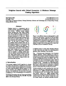
In a tree structure, top down propagated messages a basically cloned at every node which has multiple children. This results in the simple operator structure seen before. Bottom-up messages, in contrast, need to be fused. This, inherently makes the operator structure more complex. 4.1 Example For example of a graphical model’s, shown in figure (2), conditional probabilities, adapted from [4], is shown in table (1). Propagating the prior probability of the root node A down, the tree, the resultant node probabilities obtained by eigen-decomposition are given in the left column of table (1).
5 Conclusion The aim of this work has been to show that Pearl’s message passing algorithms can be viewed, not only as a fixed points of Bethe’s free energy [6], but also as solutions to a highly sparse linear set of equations. The solutions obtained by spectral decomposition and belief propagation are identical (or very similar if different boundary conditions are chosen). Actual numerical differences can also be attributed to the numerical accuracies of the spectral decomposition algorithm.
A
B
D
E
C
F
G
H
I
J
Figure 2: Example graphical model with tree topology.
Table 1: Graphical Model with Conditional Probabilities adapted from [4] (left) and computed beliefs (right) CPT Specifications Pr(A=0)=0.7 Pr(B=0 | A=0)=0.1 Pr(C=0|A=0)=0.8 Pr(D=0|B=0)=0.5 Pr(E=0|B=0)=0.3 Pr(F=0|B=0)=0.7 Pr(G=0|C=0)=0.9 Pr(H=0|C=0)=1.0 Pr(I=0|G=0)=0.2 Pr(J=0|G=0)=0.7
Pr(A=1)=0.3 Pr(B=0|A=1)=0.9 Pr(C=0|A=1)=0.2 Pr(D=0|B=1)=0.6 Pr(E=0|B=1)=0.8 Pr(F=0|B=1)=0.1 Pr(G=0|C=1)=0.0 Pr(H=0|C=1)=0.3 Pr(I=0|G=1)=0.5 Pr(J=0|G=1)=0.3
Top Down: Eigen-solution (left), Message Passing (right) Pr(A=0)=0.7 Pr(B=0)=0.34 Pr(C=0)=0.62 Pr(D=0)=0.566 Pr(E=0)=0.63 Pr(F=0)=0.304 Pr(G=0)=0.558 Pr(H=0)=0.734 Pr(I=0)=0.2798 Pr(J=0)=0.5936
Pr(A=0)=0.7 Pr(B=0)=0.34 Pr(C=0)=0.62 Pr(D=0)=0.566 Pr(E=0)=0.63 Pr(F=0)=0.304 Pr(G=0)=0.558 Pr(H=0)=0.734 Pr(I=0)=0.2798 Pr(J=0)=0.5936
Embedding the entire graph structure into a what is effectively a global transition probability in the Markov chain case, implies that the stationary distribution is sought along a “time” or iteration dimension perpendicular to the time dimension of the original Markov chain. This also makes clear that the search is done over all possible paths, since the matrix exponential is simply the limit of the sum of increasing powers of the of this global transition probability. In fact, this relationship to Feynman path integrals suggests approximations to them as methods for computing marginal beliefs. The computational efficiency of the message passing algorithm has been lost by regeneralising the problem in Ising form. However, there are two important aspects worth noting. Apart from phrasing the problem in terms of classical linear algebra and thus opening up a completely new arsenal of tools, much more is known about the behaviour of linear sets of equations subject to constraints, such as boundary problems. For instance, limit cycle phenomena, as observed in loopy belief propagation, may also have their origin in unsatisfiable constraints. Thus, the analysis of algorithms are placed on a concrete mathematical footing. The question also arises, whether new loopy belief propagation algorithms can be derived by simply looking for the largest eigenvalue solution, or whether the global transition matrix can be sampled and thus fusing graph structure search and belief propagation.
At this stage, several issues need to be solved first. In the example above we have made sure that the stationary distribution of the HMM transition probability matrix is not symmetrical. So the transpose operation, akin to a time reversal operation, is the general case. Several issues are worth noting at this stage. In the example above we have made sure that the stationary distribution of the HMM transition probability matrix is not symmetrical and that the transpose operation is also a time reversal operation [2]. Yet to be studied are time reversal for tree structures and belief operators for poly-trees.
References [1] J.M. Dixon and J.A. Tuszynski. An algorithm to obtain exact eigenvalues and eigenstates of the arbitrary spin ising hamiltonian in d dimensions. Physics Letters A, 283:300–308, 2001. [2] J.R. Norris. Markov Chains. Cambridge Series in Statistical and Probabilistic Mathematics. Cambridge University Press, 1997. [3] L. R. Rabiner. A Tutorial on Hidden Markov Models and Selected Applications in Speech Recognition. Proceeding of the IEEE, 77(2):257–284, 1989. [4] B. Ripley. Pattern Recognition and Neural Networks. Cambridge University Press, 2000. [5] G. Strang. Block tridiagonal matrices and the kalman filter. In D.X. Zhou, editor, Wavelet Analysis: Twenty Years Developments. World Scientific Press, 2002. [6] J.S. Yedidia, W.T. Freeman, and Y. Weiss. Bethe free energy, Kikuchi approximations and Belief Propagation algorithms . In NIPS, 2000.