An Optimal Fractional Order Controller for an AVR System Using Particle Swarm Optimization Algorithm Masoud Karimi-Ghartemani, Member, IEEE, Majid Zamani, Nasser Sadati, Member, IEEE, and Mostafa Parniani, Senior Member, IEEE Department of Electrical Engineering Sharif University of Technology Tehran, Iran e-mail:
[email protected],
[email protected],
[email protected],
[email protected] Abstract—Application of Fractional Order PID (FOPID) controller to an Automatic Voltage Regulator (AVR) is presented and studied in this paper. An FOPID is a PID whose derivative and integral orders are fractional numbers rather than integers. Design stage of such a controller consists of determining five parameters. This paper employs Particle Swarm Optimization (PSO) algorithm to carry out the aforementioned design procedure. A novel cost function is defined to facilitate the control strategy over both the time-domain and the frequencydomain specifications. Comparisons are made with a PID controller from standpoints of transient response, robustness and disturbance rejection characteristics. It is shown that the proposed FOPID controller can improve the performance of the AVR in all the three respects.
I. INTRODUCTION Fractional calculus extends the ordinary calculus by extending the ordinary differential equations to fractional order differential equations, i.e. those having non-integer powers of derivatives and integrals. Such equations can provide linear models and transfer functions for some infinitedimensional physical systems [1]. On the other hand, fractional order controllers may be employed to achieve feedback control objectives for such systems. Modeling and control topics using the concept of fractional order systems have been recently attracting more attentions because the advancements in computation power allow simulation and implementation of such systems with adequate precision. Fractional Order PID (FOPID) controller is a convenient fractional order structure that has been employed for control purposes [2]-[3]. An FOPID is characterized by five parameters: the proportional gain, the integrating gain, the derivative gain, the integrating order and the derivative order. Different design methods have been reported including pole distribution [4], frequency domain approach [5], state-space design [6] and two-stage or hybrid approach [7] which uses conventional (integer order) controller’s design method and then improves performance of the designed control system by adding proper fractional order controller. An alternative design method is presented in this paper based on Particle Swarm Optimization (PSO) algorithm and employment of a novel cost function which offers flexible control over time domain and frequency domain specifications. PSO is an evolutionary-type global optimization algorithm [8]-[9] which is different from well-known similar algorithms in that no operators, inspired by evolutionary procedures, are applied to the population to generate new promising solutions. PSO has already been used to determine optimal solution to 978-1-4244-1583-0/07/$25.00 ©2007 IEEE
several power engineering problems such as reactive power and voltage control [10] and state estimation [11]. We employ this algorithm to design an FOPID controller for an Automatic Voltage Regulator (AVR) problem. The proposed controller is simulated within various scenarios and its performance is compared with those of an optimally-designed PID controller. Transient response, performance robustness and disturbance rejection characteristics of both controllers are studied and superiority of the proposed controller in all three respects is illustrated. II. FRACTIONAL CALCULUS A. Definitions Fractional calculus is a generalization of the ordinary calculus. The main idea is to develop a functional operator D, associated to an order v not restricted to integer numbers, that generalizes the usual notions of derivative (for a positive v) and integral (for a negative v). Just as there are several alternative definitions for the usual integer integrals (according to Riemann, Lebesgue, Steltjes, etc.), there are also several different definitions for fractional derivatives. The most common definition is due to Riemann and Liouville [12] that generalizes the two following definitions corresponding to integer orders: c
Dx− n f ( x ) = ∫
x
c
( x − t ) n −1 f (t )dt , n ∈ , ( n − 1)!
D n D m f ( x) = D n + m f ( x), m ∈
− 0
and n, m ∈
(1) 0
(2)
The Laplace transform of D follows the well-known rules: L[ 0 Dxv f ( x)] s v F (s ) if v ≤ 0, (3) n −1 = v k v − k −1 f (0) if n − 1 < v < n ∈ s F (s ) − ∑ s 0 Dx k =0 This means that, if zero initial conditions are assumed, the systems with dynamic behavior described by differential equations involving fractional derivatives give rise to transfer functions with fractional powers of s.
B. Integer Order Approximations The most usual way of making use, both in simulations and hardware implementations, of transfer functions involving fractional powers of s is to approximate them with usual (integer order) transfer functions. One of the best-known approximations is due to Manabe and Oustaloup who use the recursive distribution of poles and zeroes. The approximating transfer function is given by [13]: 244
N
sv ≈ k∏ n =1
1 + ( s / ωz , n ) 1 + (s / ω p,n )
, v>0
of the stochastic acceleration terms that pull each particle toward pi and p g positions. The acceleration constants c1
(4)
The approximation is valid in the frequency range [ωl , ωh ] . Gain k is also adjusted so that both sides of (4) shall have unit gain at 1 rad/s. The number of poles and zeros (N) is chosen beforehand, and the desired performance of the approximation strongly depends thereon: low values result in simpler approximations, but may cause ripples in both gain and phase behaviours. Such ripples can be practically eliminated by increasing N, but the approximation will become computationally heavier. Frequencies of poles and zeroes in (4) are given by (5) ω = ω η, z ,1
l
ω p ,n = ωz ,n ε ; n = 1… N ,
(6) (7)
ωz , n +1 = ω p ,n η ; n = 1… N − 1, η = (ωh / ωl )(1− v ) / N
0.9) to wmin (of about 0.4) during a run. In general, the inertia weight w is set according to the following equation
w = wmax −
and only the latter term, i.e. sδ , needs to be approximated.
where itermax represents the maximum number of iterations, and iter is the number of current iteration or generation.
λ
III. PARTICLE SWARM OPTIMIZATION Assuming that the search space is D-dimensional, the i-th particle of the swarm is represented by the D-dimensional vector X i =(xi1 ,xi2, ...,xiD ) , and the best particle in the swarm, i.e. the particle with the smallest function value, is denoted by the index g ( p g ). The best previous position of the i-th particle is recorded and represented as P=(p , while i i1 ,pi2 ,...piD ) the position change (velocity) of the i-th particle is represented as Vi =(vi1 ,vi2 ,...,viD ) , which is clamped to a maximum velocity Vmax =(vmax1,vmax2 ,...,vmaxD ) specified by the user. Following this notation, the particles are manipulated according to the following equations: v (t +1) = wv ( t ) + c r ( p − x ) + c r ( p − x ) (11)
x
id
(t ) id
11
( t +1) id
= x +v
id
id
2 2
gd
; d = 1, … , D, xid ∈ [ xd min , xd max ]
id
(12)
where w can be expressed by the inertia weights approach [14], c1 and c 2 are the acceleration constants which influence the convergence speed of each particle [15], and r1 , r2 are random numbers in the range of [0,1]. If the velocity
vid exceeds vmaxd , then vid is limited to vmaxd . Vmax determines the resolution with which regions between the present position and the target position are searched [16]. In many experiences with PSO, Vmax is often set to the maximum dynamic range of the variables on each dimension vd max = xd max . The constants c1 and c 2 represent weightings
δ
The differential equation of a fractional order PI D controller is described by: (14) u (t ) = k e(t ) + k D −λ e(t ) + k D δ e(t ). P
I
t
D
t
The continuous transfer function of FOPID is obtained through Laplace transform and is given by: (15) G ( s ) = k + k s −λ + k s δ c
( t +1) id
(13)
A. FOPID Controller
The case v1, the approximation becomes unsatisfactory. So it is usual to split the fractional powers of s as follows (10) s v = s n s δ , v = n + δ, n ∈ , δ∈ [0,1],
id
wmax − wmin . iter itermax
IV. AVR DESIGN USING FOPID CONTROLLER
(8) (9)
ε = (ωh / ωl )v / N
and c 2 are often set to 2.0 according to the past experiences [15]. Suitable selection of inertia weight w provides a balance between global and local explorations, thus requiring less iteration to locate the optimal solution. As originally developed, w often decreases linearly from wmax (of about
P
I
D
Design of an FOPID controller involves design of three parameters k P , k I , k D and two orders λ , δ which are not necessarily integer.
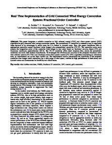
B. Linearized Model of Excitation System Automatic Voltage Regulator (AVR) is the central controller within the excitation system that maintains the terminal voltage of a synchronous generator at a specified level. Depending on the method of supplying DC power, different types of excitation systems exist [17]. As an example, we consider an alternator supplied controlledrectifier excitation system [17]. The dc regulator holds constant generator field voltage and is commonly referred to as manual control. It is primarily for testing, start-up and to cater to situations where the ac regulator is faulty. Closed loop voltage control is carried out through the ac regulator. In addition to the AVR, this loop comprises five main components, namely amplifier, exciter, excitation voltage limiters, generator and measurement and filtering. To analyze dynamic performance of AVR, transfer functions of these components are represented as follows [18]-[19]. • Amplifier model. The amplifier model is given by VR ( s) kA . = (16) VC (s ) 1 + τ A s Typical values of k A are in the range of 10 to 400. The amplifier time-constant often ranges from 0.02 to 0.1 s. • Exciter model. Exciter model and parameters greatly depend on its type.
245
Vref(s)
+
Ve VS
kP + kI s−λ + kDsδ FOPID controller
VC
VR
kA 1 + τ As
kE 1+τ Es
Amplifier
Exciter
VF 3Vf0 -3Vf0 Limiter
kG 1+τGs
Vt(s)
Generator
kR 1+τ Rs Measurement and Filter Fig. 1. Block diagram of an AVR employing an FOPID controller
A simplified transfer function of a modern exciter is VF (s ) kE = . (17) VR (s ) 1 + τ E s
Therefore, the proposed performance criterion J (k ) is defined as
J (k ) = w1 M P + w2tr + w3ts + w4 ESS
Typical values of k E are in the range of 0.8 to 1 and the time-constant τ E for an AC exciter in the range of 0.5 to 1.0 s. • Generator model. The transfer function relating the generator terminal voltage to its field voltage can be simplified to Vt ( s ) kG . = (18) VF (s ) 1 + τG s The constants are load dependent, kG may vary between 0.7 and 1.0, and τ G between 1.0 and 2.0 s from full load to no load. • Measurement model. The voltage measurement block, including PT, rectifier and filter, is often modeled with a single time constant. Vs ( s) kR . = (19) Vt (s ) 1 + τ R s
τR
ranges over 0.001 to 0.06 s. • Excitation voltage limiters. AVR and exciter output voltages are limited by windup and non-windup limiters [20]. Also, dedicated overexcitation and underexcitation limiters are employed to assure safe operation of the generator. Block diagram of the AVR compensated with an FOPID controller is shown in Fig. 1. In this figure, the combined effects of these limiters are represented by the upper and lower limits set to three times of the nominal value of the field voltage.
C. Performance Criterion In this paper, a new performance criterion in the time domain and frequency domain is proposed for evaluating the FOPID controller. This performance criterion includes the overshoot M P , rise time t r , settling time t s , steady-state error ESS , the integral of absolute error (IAE), integral of squaredinput, gain margin (GM) and phase margin (PM). Control over PM and GM guarantees robust stability of the AVR. The IAE and integral of squared-input must be computed numerically and the integral is evaluated up to T which is chosen sufficiently large so that e(t) is negligible for t > T.
T
+ ∫ ( w5 e(t ) + w6u 2 (t ))dt + 0
w7 w + 8 PM GM
(20)
where k is [ k P , k I , k D , λ , δ ] . We use the field voltage (VF) for u (t ) in (20) to prevent large values of the field current. The error e(t) is the difference between the reference voltage and the output voltage. The proposed performance criterion (20) comprises seven terms the significance of each is determined by a weight factor wi . It is up to the user to set the weight factors properly in order to attain the desired specification. For the current study, selections are w1 = 0.1 , w2 = 1 , w3 = 1 , w4 = 1 , w5 = 1 , w6 = 1 , w7 = 800 and w8 = 10 .
D. Design of FOPID Using PSO The PSO algorithm is utilized to design the controller parameters such that the controlled system exhibits desired response and robust stability as evaluated by the proposed performance criterion. The five controller parameters k P , k I ,
k D , λ and δ compose an individual (particle) k = [k P , k I , k D , λ , δ ] . The five members are assigned as real values. If there are n individuals in a population (group), then the dimension of that population is n×5. In order to limit the evaluation value of each individual of the population, J (k ) , within a reasonable range, the Routh–Hurwitz criterion is employed to test the closed-loop system stability and to get the feasible range of the coefficients of controller. A PID controller is used instead of the FOPID controller to carry out the test and to obtain the feasible range of k P , k I and k D . Also, the feasible range of λ and δ in FOPID controller is usually selected as [0 , 2]. Now we express the design steps as follows. Step 1) Randomly initialize the individuals of the population including searching points and velocities in the feasible range. Step 2) For each initial individual k of the population, calculate the values of the performance criterion in (20).
246
Step 3) Compare each individual’s evaluation value with its personal best pid . The best evaluation value among the
Step Response
1.8 1.6
pid is denoted as p g .
1.4
Step 4) Modify the member velocity of each individual k according to (11) where the value of w is set by (13). Step 5) Modify the member position of each individual k according to (12) Step 6) If the number of iterations reaches the maximum, then go to Step 7, otherwise go to Step 2. Step 7) The latest p g is the optimal controller parameter.
Amplitude
1.2 1
0.8 0.6 0.4 0.2 0 0
V. NUMERICAL RESULTS
5
10 Time (sec)
15
20
25
Fig. 2. Step response of the original AVR
B. Details of FOPID Design Using PSO for the AVR The lower bounds of the five controller parameters are zero and their upper bounds are set to kP max = 1.5 ,
kI m ax = kD max = 1 and λmax = δ max = 2 . The following parameters are used for carrying out the FOPID design using PSO: • Population size =30. • Inertia weight factor w is set as (13) where wmax = 0.9 and wmin = 0.4 . • The limit of change in velocity is set to maximum dynamic range of the variables on each dimension. • Acceleration constants c1 = 2 and c2 = 2 . • Maximum iteration is set to 500. wl and wh in (5)-(9) are set to 10-5 and 105 rad/s, • respectively. • The order of approximation in (4) is set to N=3. • T in (20) is set to 20s.
C. First Test: Basic Performance We performed 50 trials for the proposed controller. The best solution is summarized in the first row of Table I. The designed FOPID controller is of order six as its fractional derivative and integral have been approximated by N=3 in (4). The Hankel Minimum Degree Approximation (MDA) without balancing [21] can be employed to reduce its order to four 0.3381s 4 + 2.834s 3 + 4.261s 2 + 3.097 s + 1.271× 10⁻³ Gc ( s) = . 10−7 s 4 + 0.055s 3 + 13.96s 2 + 7.34 × 10⁻³ s It can further be reduced by omitting the negligible terms as 0.3381s 3 + 2.834s 2 + 4.261s + 3.097 Gˆ c ( s) = . (21) s(0.055s + 13.96)
In order to emphasize advantages of the proposed FOPID controller, we also designed a PID controller using the same method. Both Figs. 4 and 5 and Table I attest that the FOPID type AVR has better performance and higher robust stability than the PID type AVR.
D. Second Test: Robustness To examine numerically the robustness of the FOPID controller with respect to parameter uncertainties, the following simulation is performed. Assume that instead of kG = τ G = 1 , and due to the change in loading condition, the actual generator transfer function is given by Vt ( s ) 1 = . (22) VF (s ) 0.5 + s Also assume another uncertainty in the exciter model as VF (s ) 1 = . (23) VR (s ) 0.5 + 0.5s The step responses with both generator and exciter uncertainties are shown in Fig. 6. Bode Diagram
100 Original FOPID Controller
80 Magnitude (dB)
k R = 1 and τ R = 0.06 . Figures 2 show the original terminal voltage step response of the system with unity gain controller instead of FOPID controller as shown in Fig. 1.
Reduced FOPID Controller
60 40 20 0 -20 180
Phase (deg)
A. Study System Parameters A practical high-order AVR is used to verify the efficiency of the proposed FOPID controller. The system parameters are: k A = 10 , τ A = 0.1 , k E = 1 , τ E = 0.5 , V f 0 = 1 , kG = 1 , τ G = 1 ,
The Bode diagrams of the original and reduced order controllers are shown in Fig. 3, depicting very close behaviours in the frequency range of interest. Thick lines in Figs. 4 and 5 show the terminal voltage step response and Bode diagram of the AVR with the FOPID controller, respectively. Note that the simulations are performed based on the reduced-order implementation of (21) for the FOPID controller.
90
0
-90 -4 10
-2
10
0
10
Frequency (rad/sec)
247
2
10
4
10
Fig. 3. Bode diagrams of the original and reduced-order FOPID controllers TABLE I COMPARISON OF THE EVALUATION VALUES BETWEEN BOTH THE PID AND THE PROPOSED FOPID CONTROLLER
Type of Controller
kP
kI
kD
λ
δ
M P (%)
tr
ts
ESS
PM
GM
Evaluation value
FOPID Reduced FOPID PID
0.3265 ----0.10597
0.2506 ----0.0755
0.205 ----0
0.968 ----1
1.44 ----1
2 2 0
1.2 1.345 1.61
3.01 3.62 5.38
0 0 0
105 107 69.9
72.44 73.2825 8.1
19.85 20.4948 25.716
parameters. Furthermore, it can be concluded from the above simulations that the proposed FOPID controller has more robust stability and performance characteristics than the PID controller applied to the AVR.
Step Response 1.4 AVR with FOPID AVR with PID 1.2
Voltage
1
VII. REFERENCES
0.8
0.6
[1]
0.4
0.2
0 0
1
2
3
4
5 Time
6
7
8
9
10
[2]
Fig. 4. Step responses of the AVR controlled by PID and FOPID
[3]
Bode Diagram
200
AVR with PID
Magnitude (dB)
100
[4]
AVR with FOPID
0 -100
[5]
-200
Phase (deg)
-300 0
[6]
-90 -180
[7]
-270 -360
-4
-2
10
0
10
2
10
4
10
10
[8]
Frequency (rad/sec)
Fig. 5. Bode diagrams of the AVR controlled by PID and FOPID
[9]
Step Response 1.8 AVR with PID AVR with FOPID
1.6 1.4
[10]
Voltage
1.2 1
[11]
0.8 0.6
[12]
0.4 0.2 0 0
[13] 2
4
6
8
10 Time
12
14
16
18
20
[14]
Fig. 6. Terminal voltage step responses of the AVR controlled by PID and FOPID in the presence of generator and exciter uncertainties
[15]
VI. CONCLUSION
[16]
This paper presents a design method for determining the FOPID controller parameters using the PSO algorithm. The proposed method involves a new time-domain and frequencydomain performance criterion. Application of the method to a practical AVR shows that the proposed algorithm can perform an efficient search for the optimal FOPID controller
[17] [18] [19]
248
S. Canat, J. Faucher, “Fractional order: frequential parametric identification of the skin effect in the rotor bar of squirrel cage induction machine,” in Proc. of the ASME 2003 Design Engineering Technical Conf. and Computers and Information in Engineering Conf., Chicago, Illinois, USA, 2003. I. Podlubny, “Fractional-order systems and PI λ D µ controllers,” IEEE Trans. Auto. Contr. vol. 44, no. 1, pp.208-214 Jan. 1999. F. Ferreira and T. Machado, “Fractional-order hybrid control of robotic manipulators”, in Proc. of the 11th International Conference on Advanced Robotics, Coimbra, pp.393-398, June, 2003. I. Petras, “The fractional order controllers: methods for their synthesis and application”, Electrical Engineering Journal, vol. 50, no. 9-10, pp.284-288, 1999. B. M. Vinagre, I. Podlubny, L. Dorcak and V. Feliu, “On fractional PID controllers: a frequency domain approach”, in Proc. of IFAC Workshop, Terrassa, Spain, 2000. L. Dorcak, I. Petras, I. Kostial and J. Terpak, “State-space controller design for the fractional-order regulated system”, in Proc. of the ICCC 2001, Krynica, pp. 15-20. M. Chengbin and Y. Hori, “The application of fractional order PID controller for robust two-inertia speed control”, in Proc. of the 4th International Power Electronics and Motion Control Conf., Xi’an, pp.1477-1482, Aug. 2004. J. Kennedy and R. Eberhart, “Particle swarm optimization,” in Proc. IEEE Int. Conf. Neural Networks, vol. 4, pp. 1942-1947, 1995. J. J Liang, A. K. Qin, P. N. Suganthan and S. Baskar, “Comprehensive learning particle swarm optimizer for global optimization of multimodal functions,” IEEE Trans. Evol. Comp., vol. 10, no. 3, pp. 281-295, June 2006. H. Yoshida, K. Kawata, and Y. Fukuyama, “A particle swarm optimization for reactive power and voltage control considering voltage security assessment,” IEEE Trans. Power Syst., vol. 15, no. 4, pp. 1232– 1239, Nov. 2000. S. Naka, T. Genji, T. Yura, and Y. Fukuyama, “Practical distribution state estimation using hybrid particle swarm optimization,” in Proc. IEEE Power Eng. Soc., Winter Meeting, vol. 2, pp. 815–820., 2001. K. B. Oldham and J. Spanier, The Fractional Calculus, New York: Academic, 1974. A. Oustaloup, La commande CRONE: commande robuste d’ordre non entier, Herme, Paris, 1991. Y. Shi, R. Eberhart, “A modified particle swarm optimizer,” in Proc. IEEE Int. Conf. on Evolutionary Computation, pp.69-73, 1998. R. Eberhart, Y. Shi, “Particle swarm optimization: developments, applications and resources,” in Proc. IEEE Int. Conf. on Evolutionary Computation, pp.81-86, 2001. J. Kennedy, “The particle swarm: social adaptation of knowledge,” in Proc. IEEE Int. Conf. on Evolutionary Computation, pp.303-308, 1997. IEEE Standard Definition for Excitation Systems for Synchronous Machines (ANSI), IEEE Std 421.1-1986. Z. Gaing, “A particle swarm optimization approach for optimum design of PID controller in AVR system” IEEE Trans. Ener. Conver., vol. 19, no. 2, pp.384-391, June 2004. P. Kundur, Power System Stability and Control, McGraw-Hill, 1994.
[20] R. A. Krohling and J. P. Rey, “Design of optimal disturbance rejection PID controllers using genetic algorithm,” IEEE Trans. Evol. Comput., Vol. 5, pp. 78–82, Feb. 2001. [21] M. G. Safonov, R. Y. Chiang and D. J. N. Limebeer, “Optimal hankel model reduction for nonminimal systems,” IEEE Trans. on Automat. Contr., vol. 35, no. 4, pp. 496-502, April 1990.
249