An Optimization-Based Decision Support System for Strategic Planning in a Process Industry: The Case of an Aluminum Company in India Goutam Dutta Narain Gupta Robert Fourer W.P. No.2008-12-06 December 2008
The main objective of the working paper series of the IIMA is to help faculty members, research staff and doctoral students to speedily share their research findings with professional colleagues and test their research findings at the pre-publication stage. IIMA is committed to maintain academic freedom. The opinion(s), view(s) and conclusion(s) expressed in the working paper are those of the authors and not that of IIMA.
INDIAN INSTITUTE OF MANAGEMENT AHMEDABAD-380 015 INDIA
IIMA y INDIA
Research and Publications
An Optimization-Based Decision Support System for Strategic Planning in a Process Industry: The Case of an Aluminum Company in India Goutam Dutta* Narain Gupta + Robert Fourer**
Abstract
We describe how a generic multi-period optimization-based decision support system (DSS) can be used for strategic planning in process industries. The DSS is built on five fundamental elements – materials, facilities, activities, storage areas and time periods. It requires little direct knowledge of optimization techniques to be used effectively. Results based on real data from an aluminum company in India demonstrate significant potential for improvement in profits.
Key Words: Practice of OR, Decision Support Systems, Optimization, Production.
______________________________ This work has been supported by grants from the Research and Publication Committee of the Indian Institute of Management, Ahmedabad, India.
*
Professor, Production and Quantitative Methods, Indian Institute of Management, Ahmedabad, India E-mail:
[email protected] + Doctoral Student, Production and Quantitative Methods Indian Institute of Management, Ahmedabad, India
** Professor, Industrial Engineering and Management Sciences, Northwestern University, USA E-mail:
[email protected]
W.P. No. 2008-12-06
Page No. 2
IIMA y INDIA
Research and Publications
Introduction and Motivation The primary motivation for this work comes from previous work done by the authors (Fourer, 1997, Dutta and Fourer, 2004, Dutta and Fourer, 2007), in which a generic optimization based decision support system (DSS) was developed for strategic planning in process industries. This was then customized for an integrated steel plant in North America. The result was a potential increase of 16-17 % in the bottom-line of the company. It was claimed that the same approach, being generic, could be applied to other process industries. In another paper (Dutta et al. 2007), we demonstrate that the application of the same DSS in a pharmaceutical company leads to a potential increase of 3-4% in the bottom line of the company. In this paper, we strengthen our claim by demonstrating the application of the same DSS to an aluminum company in Eastern India.
The applications of linear programming based techniques to a process industry (specially the steel industry) have been many. A series of publications (Dutta et al., 1994; Sinha et al., 1995, Dutta et al., 2000) report the conceptualization, development and implementation of a mixed integer linear programming model for optimal power distribution, a project that took about 20 person years. This work resulted in a 58% increase in profitability (or a direct financial benefit of 73 million dollars) during the last six months of the fiscal year 1986-87, and accrued similar benefits in later years. However, in both the above cases, the models were customized only for the steel industry. The work on an Indian steel Company was done for a single period model; the DSS developed (Fourer, 1997, Dutta and Fourer, 2004, Dutta et al., 2007) was for a multi-period model. However, the multi period DSS was never tested with real data. In this paper we discuss the application of DSS with multi-period data.
We therefore present this optimization based DSS which is aimed at supporting strategic planning in the aluminum company. We give a brief description of previous attempts at applying OR/MS concepts in an aluminum company and discuss the basic approach of modeling in a process industry. The elements of the database required to define the mathematical model and the optimization steps are discussed in subsequent sections. In the last section of the paper, we discuss the application of the model in an aluminum company in India. The paper concludes by describing some of the experiments made on the model using real multi-period data from the company, and their results, illustrating the possible impact on the bottom-line. The mathematical formulation of our model is provided in the Appendix.
W.P. No. 2008-12-06
Page No. 3
IIMA y INDIA
Research and Publications
Review of Related Research The literature pertaining to OR/MS applications in process industries is quite diverse and a comprehensive review is beyond the scope of this paper. However, a comprehensive survey of mathematical programming models in the steel industry (Dutta and Fourer, 2001) indicates that very little work has been done in the area of planning with multi-period linear programming models.
We describe the literature on the application of OR/MS in aluminum industry. Mathematical models for operations of an ingot mill (Nicholls, 1994) and for operations of an anode manufacturing unit (Nicholls, 1995) were developed to realize the full gains of the core integrated model (Nicholls and Hedditch, 1993) of the smelter completely. The model of the ingot mill is formulated primarily in order to determine maximum throughput of the mill under varying equipment configurations such as the availability of furnaces, troughs and castors, given the maintenance schedules, and unexpected breakdowns.
An optimization method for a billet selection problem (Marsi and Warburton, 1998) was applied to analyze and improve the efficiency of aluminum extrusion at Alcan Vancouver Works, Canada. The number of distinct billet lengths and number of billets of each length to be held in inventory in order to maximize the yield are determined using the integer programming approach for a set of customer orders. The parametric analysis of grid optimizations to find the best known yields and a heuristic for billet selection problem has also been discussed.
An industrial scheduling problem is solved using the genetic algorithm approach (Gravel, et al., 2000). The algorithm proposes the best processing sequence for n orders with the sequence dependent set-up times on m parallel machines.
As already discussed above, none of the available literature focuses on multi-period models. There is also a lack of sufficient literature that discusses software development and optimal results from implementation. Hence, this paper discusses the development of a multi-material, multifacility, multi-activity and multi-period generic model that can be implemented across a spectrum of process industries.
W.P. No. 2008-12-06
Page No. 4
IIMA y INDIA
Research and Publications
Modeling a Process Industry In this section we describe our generic approach towards modeling a process industry. This approach is similar to the manner in which the authors have modeled a steel industry and a pharmaceutical industry as mentioned before (Dutta and Fourer, 2004, Dutta et al. 2007). We then go on to illustrate the application of this approach in an aluminum company.
We characterize a process industry as a network consisting of several smaller manufacturing units/machines, through which several materials are routed and processed. Normally raw materials can only be bought, and finished products can only be sold. Intermediates can often neither be bought nor sold. Practically all material can be stored as inventory. At any time, we can set products bought, sold or inventoried to zero, to indicate that no buying, selling or inventorying is possible. For each material the model also specifies a list of conversions to other materials. Each conversion has a yield and a cost at any given time. This also takes care of recycling of materials.
The production of any product is much more difficult than a simple conversion. We define a collection of facilities at which transformation occurs. At any given time, each facility houses one or more activities, which use and produce material in certain proportions.
We assume the
production system to be linear and hence we use linear optimization models. The following information is provided for each unit activity at each facility at each time:
1. The amount of each input required for an activity. 2. The amount of each output resulting from an activity. 3. The cost per unit of the activity. 4. Upper and lower limits on the number of units of each activity. 5. The number of units of activity that can be accommodated by one unit of the facility's capacity. We call this the facility-activity ratio.
In defining an activity we have two different cases. In the first case, if there is more than one product being produced at any particular facility, the production of each product is modeled as a separate activity, since each activity produces a separate output. The units of an activity may be different from the units of the facility’s capacity. For instance, the activity output might be measured in tons, but the facility’s capacity might be specified in hours. In such situations the model specifies the facility-activity ratio as tons per hour. If two products are produced at the same facility with different production rates, we have two different activities and two different
W.P. No. 2008-12-06
Page No. 5
IIMA y INDIA
Research and Publications
facility-activity ratios. In the other case, if a facility has essentially only one activity, both the activity and the facility capacity may be in the same units. The facility-activity ratio must be unity in this case.
Another important factor in the model is the definition of time. We take the time unit to be flexible from one day to one year. For long term capital budgeting and business planning, we would use a year, month or quarter as the unit of time, whereas for the short-term operational model, we use one week or one day as the unit of time. In the current case we have taken the unit of time to be one month as we attempt to provide long-term strategic support. With respect to strategic planning, the DSS is intended to help answer questions such as the following:
1. What is the optimal product mix and how does it compare with the current product mix? 2. Which products should be chosen for addition to the existing products with the same facility? 3. What is the effect of cost or price changes, of raw materials or finished products, on the product mix and overall profit?
Model Formulation We optimize a generalized network-flow linear program based on five fundamental elements: materials, facilities, activities, storage areas and time periods. The details of the computer implementation are beyond the scope of this paper and are discussed in another paper (Dutta and Fourer, to appear, 2008). An appendix to this paper shows the model’s complete formulation. Definitions The fundamental elements are defined as follows: Times: These are the periods of the planning horizon and are represented by discrete numbers 1, 2, 3 . . . T. Materials: Any product in the manufacturing unit at any stage of production — input, intermediate, output — is regarded as a material. Facilities: A facility is a collection of machines which produce some materials from others. For example, a pre-heater, bliss mill, hot mill are facilities. Activities: At any given time, each facility houses one or more activities, which use and produce material in certain proportions. In each activity at each time, we have one or more input materials being transformed into various output materials.
W.P. No. 2008-12-06
Page No. 6
IIMA y INDIA
Research and Publications
Storage Areas: These are the places where raw materials, intermediate products, and finished products can be stored.
The model is a generalized network-flow model that maximizes the contribution to profit (nominal or discounted) of a company, subject to the following categories of constraints for all time periods: 1. Material balances 2. Facility capacities — optionally “soft” capacities that may be exceeded at some cost in outsourcing 3. Storage area capacities 4. Bounds — on material (bought, sold, inventoried), on facility inputs and outputs, and on activities
Owing to the generality of the model, each material can potentially be bought, sold, or inventoried at each time period. Thus any material can be modeled as a raw material, intermediate, or finished product depending on the circumstances being considered.
Model Assumptions The model we describe is general enough to accommodate facilities that are in series, in parallel, or in some more complex configuration. As previously remarked, each facility can have one or more activities.
There can be purchase, sale and storage of materials at the raw materials stage, at the finishing stage or at the intermediate processing stages. Moreover, the purchase price of raw materials, the selling price of finished goods, and the inventory carrying costs may vary over time.
At any given time, one or more materials may be used as inputs or outputs at a facility. Generally more than one input material is used to produce one output. The relative proportions of inputs and outputs (the technological coefficients) of an activity remain the same in a given period. Technological coefficients may vary with time.
The capacity of each facility and each storage area is finite. Since the facilities will have different patterns of preventive maintenance schedules, the capacities of the facilities will vary over time.
W.P. No. 2008-12-06
Page No. 7
IIMA y INDIA
Research and Publications
Costs and production amounts are considered to vary proportionately with activity levels. Thus the essential features of the production-planning problem can be captured in a deterministic, linear optimization model.
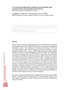
Implementation Our model is implemented within 4th Dimension (Adams and Becket, 1999), a relational database management system. Other database systems such as Access or Oracle could be used just as well. The Figure 1 shows the structure of the database as expressed within 4th Dimension. The five boxes labeled Materials, Facilities, Activities, Times, and Storage_Areas correspond to the five major elements or files of the database. Items within each box denote the file’s data fields and subfiles, with the subfile entries distinguished by a light-shaded line that runs to the top of a separate box in which the subfile data fields are listed. The smaller, independent database structure in the upper middle of the diagram holds a generated linear program as described in the next subsection.
The following 4th Dimension’s notation, we use bracketed names to denote files and apostrophes to separate subfile and field names. Thus [Facilities] is the database file of facilities, [Facilities]Inputs is the subfile of facility inputs, and [Facilities]Inputs’InMin is a data field of the subfile. Further details can be found in the discussion of the one-period model in an earlier publication (Fourer, 1997).
W.P. No. 2008-12-06
Page No. 8
IIMA y INDIA
Research and Publications
Figure 1: Database structure for the general planning model.
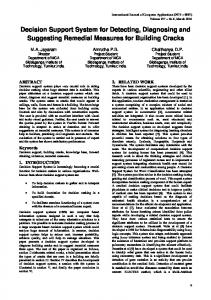
Optimization Steps Once the data of the five database files and their respective sub-files are entered, they are validated by a set of diagnostic tests Dutta et al. (to appear, 2008). This subsection describes how the subsequent optimization process is carried out. The principal steps (Figure 2) are as follows:
1. The data describing the production scenario at different time periods are collected and stored in the database. 2. The constraints associated with the linear program are generated. The constant terms of the constraint equations or inequalities, LoRHS and HiRHS, are extracted from the database and stored in the [Constraints] file
W.P. No. 2008-12-06
Page No. 9
IIMA y INDIA
Research and Publications
Figure 2: Optimization steps.
3. The variables of the associated linear program are determined, along with their coefficients in the constraints. Variables are stored in a separate [Variables] file and coefficients in the [Variables]Coeff subfile. This step gives the user a choice of discounted or undiscounted optimization. If the latter is chosen then it prompts for an interest rate, and all the cost, price, and revenue data are converted to their discounted values in the objective function. 4. The [Constraints] and [Variables] files are scanned and all of the essential information about the linear program is written to an ordinary text file in a compact format. This text file is the input file to our solver. 5. A linear programming solver reads the text file—we used XMP (Martsen, 1981) — which solves the indicated linear program and then writes the optimal values of the variables to a second text file. 6. The second text file is read and the optimal values are placed in appropriate fields of the [Materials], [Facilities], [Activities], and [Storage_Areas] files and their subfiles.
To support these activities the database offers three modes of display. The Data mode is primarily for entering data describing the operations to be modeled. The Optimal mode also shows the fields for the optimal values, and hence is intended for examination of results. Finally, an Update mode allows small changes to be made to the data without a time-consuming re-generation of the [Constraints] and [Variables] files.
W.P. No. 2008-12-06
Page No. 10
IIMA y INDIA
Research and Publications
Application to an Aluminum Company The company is one of the largest aluminum processing companies of eastern India. The annual turnover of the company is $70 million. The total annual production of aluminum based products is 30,000 tons. The aluminum model consists of 569 materials, 17 facilities, and 568 activities.
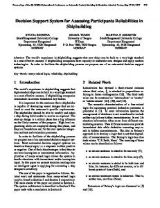
The basic raw material used for aluminum products is aluminum ingots. The company is engaged in the production of a total of 95 final products with different compositions, sizes, shapes, and prices. The planning horizon is annual, however the DSS is generic to consider any other time horizon like monthly or quarterly planning. The company’s characteristics and variability in the data are portrayed in the next section. The raw material is transformed at collections of facilities such as SMS Mill, Bliss Mill, Scalper, Pre-Heater, Shearer etc. The process flow diagram of the production of aluminum based products is presented in Figure 3.
Conversion of the Company’s Data to Model Data Due to reasons of confidentiality, the actual names of products and facilities were replaced by code-names. The yield, capacity and facility activity ratios were the annual average values for the previous year. The exact input and output materials of each facility, yields for each activity, and capacities for different machines were supplied. All of the results are based on the data presented to us in this disguised format.
Since the route of each product is different, the products at different stages were distinctly identified as different materials or different records in the [Materials] file. The facilities include scalper, pre-heater, hot mill, SMS mill, bliss mill, homo annealing, slitting, cutting, rolling units, and final shearing units. We decided to keep the unit of measurement of all materials in tons and time period of planning in years.. The capacity of each facility was in hours and the capacity of each activity was also kept in tons. The facility-activity ratio was thus expressed in tons per operating hour. The company did not supply a corresponding minimum number of operating hours, so [Facilities] FacTime'CapMin was set to zero.
Contact Points To check that the model represents reality, contact points have been identified. These points are functions of the variables in the model and at the same time measurable quantities in real life. We consider the following figures and their respective units:
W.P. No. 2008-12-06
Page No. 11
IIMA y INDIA
Research and Publications
1. Total production of the aluminum unit (tons) 2. Total revenue (US dollar) 3. Total cost of purchases (US dollar) 4. Total cost of activities (US dollar) 5. Total cost of inventory carrying (US dollar) 6. Total net profit (US dollar)
By comparing these quantities, we were able to verify that the results of the model were in line with the capabilities of the plant.
Company Characteristics and Variability of Data We present the scale of operation and variability in the planning parameters in the aluminum company; see Table 1. It is evident that there is wide variability in the sale prices and market demand of final products, and purchase prices of the raw materials. The integrated multi-period aluminum planning model has 8,858 decision variables under a set of 6,654 constraints. The number of non-zeros (intersecting element of a pair of a constraint and a variable) in the model is 26,844 with 0.05% sparseness. Variability in the rate of production and cost of production presented in Table 1, also demonstrates the potential of optimization in the aluminum company.
Table 1: Company Characteristic and Variability in Data Parameters Minimum Maximum Sell Price 2340.94 $ 5698.81 $ Market Demand 6.30 tons 2,568.30 tons Range of Facility Activity Ratio (Tons/Hour) 0.04 20.42 Range of Activity Cost (US $ /Ton) 1.84 1209.05 Number of Variables 8589 Number of Constraints 6654 Number of Coefficients 26844 Sparseness (Model Density) 0.05 % Fundamental Elements of the Model Number of Materials 569 Number of Facilities 17 Number of Activities 568 Number of Planning Horizons 3 Number of Intermediates 473 Number of Finished Goods 95
W.P. No. 2008-12-06
Page No. 12
IIMA y INDIA
Research and Publications
MILLING
ROLLING INGOT
Process flow PRE HEATER
VIRGIN METAL + SCRAP
REMELT
INGOT SAW HOT MILL
CONCAST COIL/ HRC
SMS MILL
CHOPPING SLITTER
YYYYY CUT TO LENGTH
BLISS MILL
BATCH ANNEALING FURNACE
FLAT MILL
ROLL FORMER
SHEAR
CIRCLE PUNCHING CIRCLE SHEAR
INSPECTION
WAREHOUSE & DESPATCH
Figure 3: A Process Flow Diagram of Aluminum Company
Experiments with the DSS We design and implement the following experiment on single period and multiple period planning models. We optimize with the company’s actual production limits for the previous financial year. We also find the final products for which optimal values are at their upper limits ([Materials]MatTime'SellOPT= [Materials]MatTime'SellMax). We increase the upper bound by 5% for each final product. We re-run the optimization model and note the optimal results of the model. We repeat the same procedure twice with an additional 5% increase each time.
Thus we consider the following four cases: Case 0
: With the company’s upper and lower bounds
Case 1
: With the company’s upper bounds increased by 5% over case 0
Case 2
: With the company’s upper bounds increased by 5% over case 1
Case 3
: With the company’s upper bounds increased by 5% over case 2
% Change
: Indicates the percentage improvement of case 3 over case 0
The results of this experiment are shown in Table 2 and 3 for single period and multiple period planning respectively. The experiment addresses the following issues. 1. What is the opportunity for increasing the profit of the company? 2. Which facilities have the most costly capacity limitations? W.P. No. 2008-12-06
Page No. 13
IIMA y INDIA
Research and Publications
3. What are the processes that need the attention of the management? We also discuss the difficulties involved and indicate the impact that the DSS can make in improving the bottom line of a company.
Impact of Optimization We present all the results of the application in the aluminum company in US Dollars. We apply an exchange rate of Rs. 40 per US Dollar. We maintain consistency in presenting all the results. Impact of Single Period Optimization We demonstrate the impact of single period (one year) optimization in the aluminum company (Table 2). We outline the following observations from these results: 1. An increase of net (contribution to) profit by 7.74%. 2. The rate of increase of total revenue is higher than the rate of increase of total cost of activity. 3. The unit revenue and unit cost of activity is lower by 0.10%, and 1.80% respectively. 4. The rate of reduction of unit cost of activity is higher than the rate of reduction of unit revenue. 5. The unit cost of purchase remains unchanged. The total quantity to be purchased for raw materials is bounded by company constraints. The increase in market bounds changes the optimal product mix but does not alter the amount of raw material purchases. In Table 2, we observe an increase in all the contact points on an absolute basis. An increase in all the contact points may lead to a confusion that the increase in total profit is because of an increase in total production. We also determine the profit per unit, and observe an increase of 3.57%. This indicates that the increase in profit is not just because of an increase in total production but also due to the change in the physical route that the final products follow in the network of facilities. Table 2: Results of Experiment in Single Period Aluminum Model
Cases --> Total Revenue Cost of Purchases Cost of Activities Net Profit Total Aluminum
Unit Million $ Million $ Million $ Million $ Tons
Revenue Cost of Purchase Cost of Activity Net Profit
US $ US $ US $ US $
Grand Summary Case 0 Case 1 Case 2 87.49 88.58 89.31 52.27 52.89 53.22 25.00 25.21 25.35 10.22 10.48 10.74 26135.61 26446.00 26611.98 Unit Basis Summary 3347.56 3349.42 3356.12 2000.00 2000.00 2000.00 956.64 953.24 952.51 390.92 396.18 403.62
W.P. No. 2008-12-06
Case 3 90.93 54.38 25.54 11.01 27188.13
% Change 3.93% 4.03% 2.16% 7.74% 4.03%
3344.32 2000.00 939.43 404.89
-0.10% 0.00% -1.80% 3.57%
Page No. 14
IIMA y INDIA
Research and Publications
Impact of Multi-period Optimization We presented and examined the results of multi-period (three year) optimization in the aluminum company. We conduct the experiment on an integrated multi-period aluminum model (Table 3). We outline the following observations from the results of experiments:
1. The net (contribution to) profit increases by 6.72%. An increase of 6.72% in the existing profit of $41.86 million is a significant improvement. 2. The sum of increase in cost of purchases ($6.68 million), cost of activities ($1.83 million), and cost of inventory carrying ($0.39 million) is equal to $8.9 million, which is relatively lower than the increase in total revenue ($11.73 million). This explains the increase in net (contribution to) profit. 3. It is interesting to note that all unit basis cost components except cost of purchases show a decrease, while net unit profit shows an increase of 2.40%. This verifies our argument that the increase in profit is not solely because of increase in production but also due to a change in the optimal product mix. 4. Table 3: Result of Experiment, Increased Market Bounds in Aluminum Model Grand Summary: Multiple Period Optimization Unit Case 0 Case 1 Case 2 Case 3 Million $ 289.27 293.94 297.48 301.00 Million $ 158.46 161.13 162.97 165.14 Million $ 13.95 14.46 14.60 14.34 Million $ 75.01 75.59 76.20 76.84 Million $ 41.86 42.77 43.71 44.67 Tons 79,230 80,566 81,484 82,569 Unit Basis Summary US $ 3651.02 3648.44 3650.78 3645.44 Revenue US $ 2000.00 1999.98 2000.02 2000.02 Cost of Purchase US $ 176.07 179.48 179.18 173.67 Cost of Inv Carrying US $ 946.74 938.24 935.15 930.62 Cost of Activity US $ 528.34 530.87 536.42 541.00 Net Profit Cases --> Total Revenue Cost of Purchases Cost of Inv Carrying Cost of Activities Net Profit Total Aluminum
% Change 4.06% 4.22% 2.80% 2.44% 6.72% 4.22% -0.15% 0.001% -1.36% -1.71% 2.40%
Extension for Future Research We have studied a generic model for process industries that is multi-period, multi-facility and multiple-activity, and that optimizes the nominal or discounted net profit of a company subject to the constraints of the industry. The problem can be visualized either as a multi-period single scenario or a single period multi-scenario. We would like to extend it to multi-period, multiscenario model. This requires that we define some of the data as stochastic, with probability
W.P. No. 2008-12-06
Page No. 15
IIMA y INDIA
Research and Publications
distributions. This will be a more difficult problem as the constraint generation and variable generation time will increase proportionately with the number of scenarios. We have already started working on this problem and doctoral work (Gupta, 2008) provides the details of such extension.
A second extension of the model will be studying the non-linearity of the model. As some of the industrial cost curves are non-linear or at best can be represented as having piecewise linear behavior, it may be worthwhile to study such extension.
A third extension will be to have multiple–objective linear programs and represent them in the database. This can be done by changing the model management system. For example, the current model can be changed to cost minimization, revenue maximization and maximization of marketable products or maximization of the utilization of marketable products (revenue or production). It is possible to have menu driven interfaces which allow for optimization over different objectives.
A fourth extension will be to attempt this DSS with respect to another process industry. We have used the model for the steel, pharmaceutical and aluminum industries. We need to test the model with real data from another process industry. In a developing country like India, we have a number of process industries. We need to test the DSS with other important process industries like copper, food, and fertilizers.
W.P. No. 2008-12-06
Page No. 16
IIMA y INDIA
Research and Publications
References Adams D and Beckett D (1999). Programming in 4th dimension, the ultimate guide, automated solutions group: Huntington Beach, CA, U.S.A. Dutta G, Sinha G P, Roy PN, and Mitter N (1994). A linear programming model for distribution of electrical energy in a steel plant. International Transactions in Operational Research, 1(1): 1729. Dutta G and Fourer R (2001) A survey of linear programming applications in an integrated steel plant. Manufacturing and Service Operations Management, 3(4): 387-400. Dutta G and Fourer R, (To Appear, 2008). Database structure for a class of multi-period mathematical programming models. Accepted in Decision Support Systems. Dutta G and Fourer R (2004). An optimization based decision support system for strategic and operational planning in process industries. Optimization and Engineering 5(3):295-314. Dutta G, Fourer R, Majumdar A and Dutta D (2007). An optimization based decision support system for strategic and operational planning within process industries: case of pharmaceuticals industry in India. International Journal of Production Economics 102: 92-103. Fourer R (1997) Database structure for mathematical programming models. Decision Support Systems. 20: 317-344. Gravel, Marc, Price, Wilson L, and Gagne, Caroline. (2000) Scheduling jobs in an alcan aluminum foundry using a genetic algorithm. International Journal of Production Research 38: 3031-3041. Gupta, N (2008) A stochastic optimization based decision support system for strategic planning in process industries. PhD Dissertation, IIM Ahmedabad, India. Nicholls, Miles G (1995). Aluminum production modeling - a nonlinear bi level programming approach. Operations Research 43: 208-218. Helmberg, Christoph (1995). Cutting aluminum coils with high length variabilities”, Annals of Operations Research 57: 175-189. Marsten RE (1981). The design of XMP linear programming library. ACM Transactions on Mathematical Software. 7: 481-497. Nicholls, M G and Hedditch, D J (1993). The development of an integrated mathematical model of an aluminum smelter. Journal of the Operational Research Society 44: 225-235. Nicholls, MG (1994) Optimizing the operations of an ingot mill in an aluminum smelter. Journal of the Operational Research Society 45: 987-998. Nicholls, Miles G and Criteria (1995). Scheduling production in a heavily constrained plant-anode manufacture in an aluminum smelter. Journal of the Operational Research Society 46: 579-591.
W.P. No. 2008-12-06
Page No. 17
IIMA y INDIA
Research and Publications
Nicholls, Miles G (1997). Developing an integrated model of an aluminum smelter incorporating sub-models with different time bases and levels of aggregation. European Journal of Operational Research 99: 479-492. Rodrigo, Renuka, and Nicholls, Miles G (1996). The development of an integrated model for the optimization of the operations of a reduction cell in aluminum smelting. Australian Society of Operations Research Bulletin 15: 2-11. Sinha G P, Chandrashekaran BS, Mitter N, Dutta G, Singh SB, Roy PN and Roy Choudhary A (1995). Strategic and operations management with optimization at tata steel. Interfaces, 25(1) Stadtler, Hartmut (1990). A one-dimensional cutting stock problem in the aluminum industry and its solution. European Journal of Operational Research 44: 209-223. Warburton. A and Masri K (1998). Using optimization to improve the yield of an aluminum extrusion plant. Journal of the Operational Research Society 49: 1111-1116. Walker LJ and Woolven JD (1991). Development and use of a visual interactive planning board within alcan aluminum. European Journal of Operational Research 54: 299-305.
W.P. No. 2008-12-06
Page No. 18
IIMA y INDIA
Research and Publications
Appendix Model Formulation We first define the data, in five parts: times, materials, facilities, activities, and storage-areas. The notation for the decision variables is then presented. Finally the objective and constraints are described, in both words and formulae.
All quantities of materials are taken to be in the same units, such as kilograms. Time data T= {1,……,T} is the set of time periods in the planning horizon, indexed by t ρ is the interest rate per period, taken as zero if there is no discounting Materials data M is the set of all materials
l
buy jt
u c l
jt
buy jt
sell jt
u c l
buy
sell jt
sell jt
inv jt
u
inv jt
v
inv
c
inv
j0
jt
= lower limit on purchases of material j, for each j∈M and t∈T
= upper limit on purchases of material j, for each j∈M and t∈T
= cost per unit of material j purchased, for each j∈M and t∈T
= lower limit on sales of material j, for each j∈M and t∈T
= upper limit on sales of material j, for each j∈M and t∈T
= revenue per unit of material j, for each j∈M and t∈T
= lower limit on inventory of material j, for each j∈M and t∈T
= upper limit on inventory of material j, for each j∈M and t∈T
= initial inventory of material j, for each j∈M
= holding cost per unit of material j, for each j∈M and t∈T
W.P. No. 2008-12-06
Page No. 19
IIMA y INDIA
M
conv
Research and Publications
⊆ {j∈M, j′∈M : j ≠ j′} is the set of conversions: (j,j′)∈
α
conv jj ′t
conv
M
means that material j can be converted to material j′
= number of units of material j′ that result from converting one unit of material j,
for each (j,j′)∈
c
conv jj ′t
M
conv
, t∈T
= cost per unit of material j of the conversion from j to j′, for each (j,j′)∈
M
conv
,
t∈T
Facilities data F is the set of facilities
l
cap it
= the minimum amount of the capacity of facility i that must be used, for each i∈F and t∈T
u
c
cap it
cap it
= the capacity of facility i, for each i∈F and t∈T = the cost of vendoring (outsourcing) a unit of capacity at facility i, for each i∈F and t∈T
F
in
⊆ FxM is the set of facility inputs: (i,j)∈
l
in
F
in
means that material j is used as an input at facility i
= the minimum amount of material j that must be used as input to facility i, for
ijt
each (i,j)∈
u
in ijt
out
in
, t∈T
= the maximum amount of material j that must be used as input to facility i, for each (i,j)∈
F
F
F
in
, t∈T
⊆ FxM is the set of facility outputs: (i,j)∈
F
out
means that material j is produced as an output at facility i W.P. No. 2008-12-06
Page No. 20
IIMA y INDIA
l
out ijt
Research and Publications
= the minimum amount of material j that must be produced as output at facility i, for each (i,j)∈
u
out ijt
F
out
, t∈T
= the maximum amount of material j that must be produced as output at facility i, for each (i,j)∈
F
out
, t∈T
Activities data act
F
⊆ {(i,k) : i∈F} is the set of activities: (i,k)∈
l
act ikt
act ikt
act ikt
r
ikt
act
means that k is an activity available at facility i
F
act
, t∈T
= the maximum number of units of activity k that may be run at facility i, for each (i,k)∈
c
act
= the minimum number of units of activity k that may be run at facility i, for each (i,k)∈
u
F
F
act
, t∈T
= the cost per unit of running activity k at facility i, for each (i,k)∈
in
act
, t∈T
= the number of units of activity that can be accommodated in one unit of capacity of facility i, for each (i,k)∈
A
F
⊆ {(i,j,k,t) : (i,j)∈ (i,j,k,t)∈
in
A
F
in
(i,k)∈
F
act
F
act
, t∈T
, t∈T} is the set of activity inputs:
means that input material j is used by activity k at facility i during
time period t
α
in ijkt
= units of input material j required by one unit of activity k at facility i in time period t, for each (i,j,k,t)∈
out
A
⊆ {(i,j,k,t) : (i,j)∈
F
out
in
A
(i,k)∈
F
act
, t∈T} is the set of activity outputs:
W.P. No. 2008-12-06
Page No. 21
IIMA y INDIA
(i,j,k,t)∈
Research and Publications out
A
means that output material j is produced by activity k at facility i
during time period t
α
out ijkt
= units of output material j produced by one unit of activity k at facility i in time period t, for each (i,j,k,t)∈
out
A
Storage-areas data S is the set of storage areas
l
stor st stor
u
st
= lower limit on total material in storage area s, for each s∈S, t∈T = upper limit on total material in storage area s, for each s∈S, t∈T
Variables buy
x
jt
x
sell
x
stor
x
inv
x
inv
x
conv
x
in
jt
jst
jt
j0
jj ′t
ijt
out
x
ijt
x
ikt
x
it
act
cap
= units of material j bought, for each j∈M, t∈T
= units of material j sold, for each j∈M, t∈T
= units of material j in storage area s, for each j∈M, s∈S, t∈T
= total units of material j in inventory (storage), for each j∈M, t∈T
= initial inventory of material j, for each j∈M
M
= units of material j converted to material j′, for each (j,j′)∈
= units of material j used as input by facility i, for each (i,j)∈
conv
F
in
, t∈T
= units of material j produced as output by facility i, for each (i,j)∈
= units of activity k operated at facility i, for each (i,k)∈
F
act
, t∈T
F
out
, t∈T
, t∈T
= units of capacity vendored at facility i, for each i∈F, t∈T
W.P. No. 2008-12-06
Page No. 22
IIMA y INDIA
Research and Publications
Objective Maximize the sum over all time periods of revenues from sales less costs of purchasing, holding inventories, converting, operating activities at facilities and vendoring:
∑ (1+ ρ )
−t
Z (t )
t ∈T
where,
∑c x
Z(t) =
sell
sell
jt
jt
j∈M
j∈M
∑c x
-
i∈ F
∑c x
-
cap
cap
it
it
buy
buy
jt
jt
-
∑c x
j ∈M
inv
inv
jt
jt
∑ c x
-
( j , j ′ )∈
M
conv
conv
jj ′t
jj ′t
conv
-
∑c x
( i , k )∈
F
act
act
ikt
ikt
act
Constraints For each j∈M, r∈R and t∈T, the amount of material j made available by purchases, production, conversions and beginning inventory must equal the amount used for sales, production, conversions and ending inventory: buy
x
∑ x
+
jt
( i , j )∈
∑ x
( j , j ′ )∈
M
conv
F
conv
F
+
∑ α x
( j ′, j )∈
x
+
jj ′t
For each (i,j)∈
out
out ijt
in
M
conv
conv
conv
j ′jt
j ′jt
+
x
inv jt −1
=
x
sell jt
+
∑ x
( i , j )∈
F
in
in ijt
+
inv jt
and t∈T, the amount of input j used at facility i must equal the total
consumption by all the activities at facility i:
x
in ijt
=
∑ α x
( i , j , k , t )∈
For each (i,j)∈
A
in
F
out
in
act
ijkt
ikt
and t∈T, the amount of output j produced at facility i must equal the total
production by all the activities at facility i:
x
out ijt
=
∑ α x
( i , j , k , t )∈
A
out
out
act
ijkt
ikt
W.P. No. 2008-12-06
Page No. 23
IIMA y INDIA
Research and Publications
For each i∈F and t∈T, the capacity used by all activities at facility i must be within the range given by the lower limit and the upper limit plus the amount of capacity vendored:
l
cap
∑x /r
≤
it
( i , k )∈
act
act
ikt
ikt
act
F
≤
u
cap it
+
x
cap it
For each j∈M, the amount of material inventoried in the plant before the first time period is defined to equal the specified initial inventory:
x
inv
v
=
j0
j0
For each j∈M and t∈T, the total amount of material j inventoried is defined as the sum of the inventories over all storage areas:
∑x s∈S
stor
x
=
jst
inv jt
For each s∈S and t∈T, the total of all materials inventoried in storage area s must be within the specified limits:
l
stor st
∑x
≤
j∈M
stor
≤
jst
u
stor st
All variables must lie within the relevant limits defined by the data:
l
buy
l
sell
l
inv
jt
buy
≤
x
≤
x
jt
x
0≤
x
conv
0≤
x
0≤
x
stor
in
≤
x
≤
x
l l
ij
out ij
cap
jt
jt
≤
buy
≤
u
≤
u
u
inv jt
jt
sell jt
,
,
for each j∈M and t∈T
,
for each j∈M and t∈T
for each j∈M and t∈T
,
jj ′t
it
sell
inv
≤
jt
jt
for each (j,j′)∈
M
conv
and t∈T
,
for each i∈F and t∈T
,
for each s∈S, j∈M and t∈T
jst
in ij
out ij
≤
u
≤
in ij
u
, out ij
,
for each (i,j)∈
F
in
for each (i,j)∈
F
out
and t∈T
and t∈T
W.P. No. 2008-12-06
Page No. 24
IIMA y INDIA
l
act ik
≤
x
act ik
Research and Publications
≤
u
act ik
,
for each (i,j)∈
F
act
and t∈T
Figure Captions Figure 1: Database structure for the general planning model Figure 2: Optimization steps Figure 3: A Process Flow Diagram of an Aluminum Company
Table Captions Table 1: Company Characteristic and Variability in Data Table 2: Results of Experiment in Single Period Aluminum Model Table 3: Result of Experiment, Increased Market Bounds in Aluminum Model
W.P. No. 2008-12-06
Page No. 25