AN OPTIMIZED FORWARD MODEL AND RETRIEVAL SCHEME FOR MIPAS NEAR REAL TIME DATA PROCESSING Marco Ridolfi1, Bruno Carli1, Massimo Carlotti2, Thomas von Clarmann3, Bianca M. Dinelli4, Anu Dudhia5, Jean-Marie Flaud6, Michael Höpfner3, Paul E. Morris5, Piera Raspollini1, Gabriele Stiller3 and Robert J. Wells5 1
IROE – CNR, Via Panciatichi, 64 I-50127 Firenze (Italy), Email:
[email protected] 2 Dip. Chimica Fisica e Inorganica Università di Bologna, V.le Risorgimento, 4 I-40136 Bologna (Italy), Email:
[email protected] 3 Forschungszentrum Karlsruhe GmbH, Institut fuer Meteorologie und Klimaforschung, Postfach 3640, D-76021 Karlsruhe, FRG (Germany), Email:
[email protected] 4 ISM - CNR Via Gobetti, 101 I-40129 Bologna (Italy), Email:
[email protected] 5 Department of Atmospheric, Oceanic and Planetary Physics, Oxford University, Claredon Laboratory, Parks Road, OXFORD, OX1 3PU - United Kingdom, Email:
[email protected] 6 Laboratoire de Photophysique Moleculaire, Université de Paris Sud, Bat 213, Campus d'Orsay, F-91405 Orsay CEDEX – France, Email:
[email protected]
ABSTRACT The infrared emission limb sounder MIPAS (Michelson Interferometer for Passive Atmospheric Sounding) will be operated as an ESA core instrument on the ENVISAT-1 satellite. Near real time retrieval of pressure, temperature (p,T) and volume mixing ratio (VMR) of six key species (O3, H2O, HNO3, CH4, N2O and NO2) from calibrated spectra will be performed in the Level 2 processor of the ENVISAT Payload Data Segment. An ESA supported study was carried out for the development of an optimized (with respect to speed and accuracy) retrieval algorithm suitable for the implementation in MIPAS Level 2 processor. In the framework of this study, an optimized forward / retrieval code was implemented based on the global fit approach. In this approach all the spectra of a limb-scanning sequence are simultaneously fitted in order to correctly account for error correlations in the altitude domain. Besides, only spectral intervals which are sensitive to the retrieved parameters are analyzed by using a microwindow approach. This also minimizes interferences of spectral signatures from atmospheric species with unknown concentration. Finally, a sequential retrieval of the target species VMR profiles is performed. The trade-off between run time and accuracy of the retrieval was optimized from both the physical and mathematical point of view, with optimizations in the program structure, in the radiative transfer model and in the computation of the retrieval Jacobian. The attained performances of the retrieval code are: noise error on temperature < 2 K at all the altitudes covered by the typical MIPAS scan (8-53 km with 3 km resolution), noise error on tangent pressure < 3 % , noise error on VMR of the target species < 5 % at most of the altitudes covered by the standard MIPAS scan. The run-time required to perform p,T and VMR retrieval of the five MIPAS target species from a limb-scanning sequence of 16 limb-views is less than 1 minute on a modern work-station.
1. INTRODUCTION MIPAS (Michelson Interferometer for Passive Atmospheric Sounding) is an ESA developed instrument to be operated on board the ENVISAT-1 satellite. It will perform limb sounding observations of the atmospheric emission spectrum in the middle infrared region, from which concentration profiles of atmospheric constituents will be derived on a global scale over a period of several years. Since atmospheric emission in the middle infrared is strongly dependent on the temperature and, in general, limb observations are strongly affected by the observation geometry, a correct interpretation and analysis of the observed spectra require a good knowledge of these quantities, that have to be determined for each limb scan sequence. The pressures at the tangent altitudes (characterizing the observation geometries) and the temperature profile (p,T), as well as the volume mixing ratio (VMR) profiles of six high priority species (O3, H2O, HNO3, CH4, N2O and NO2), will be routinely retrieved in near real time (NRT). The retrieval of these parameters from calibrated spectra (Level 1b data) is indicated as NRT Level 2 processing. A scientific code for NRT Level 2 analysis, suitable for implementation in ENVISAT Payload Data Segment and optimized for the requirements of speed and accuracy has been developed in the frame of an ESA supported study. The
scientific code is called Optimized Retrieval Model (ORM) and includes two separate components for p,T and VMR retrievals respectively. The required accuracy performances of the retrieval code are the following ones: • Temperature noise error < 2 K at all the altitudes covered by the standard MIPAS scan (8-53 km) • Tangent pressure noise error: < 3% • Noise error on the retrieved VMR of the key species: < 5 % at all the altitudes covered by the standard MIPAS scan. The required run-time to perform p,T and VMR retrieval of the five MIPAS target species from a limb-scanning sequence of 16 limb-views should be less than 1 hour on a SUN SPARCstation 20. In order to meet the above accuracy and speed requirements, several mathematical and physical optimisations have been implemented in the retrieval model and the performance improvements have been verified on the basis of simulated test scenarios. In this paper, after the description of the general features of the retrieval model (Sect. 2) and of the optimisations implemented in both the forward model and Jacobian calculation (Sect. 3 and 4), we will focus on the validation tests that have been performed so far (Sect.5) and on the accuracy and run-time performances of the developed algorithm (Sect. 6 and Sect. 7).
2. THE INVERSION METHOD The instrument observes the radiance emitted by the atmosphere at different values of the spectral frequency and the limb-viewing angle. The dependence of the spectra on the unknown profiles is not linear, so that an analytical expression for the solution cannot be found. A theoretical model, called forward model, simulates the observations through a set of parameters, i.e. the atmospheric profiles that have to be retrieved. The inversion method consists in the search for the set of values of the parameters that produce the ‘best’ simulation of the observations. The Non Linear Least Square Fit is adopted for the retrieval algorithm [1], [2], i.e. the solution is the profile that minimizes the χ 2 function, given by the square summation of the difference between observation and simulations, weighted by the measurement noise. This solution is found by means of an iterative procedure, using the Gauss-Newton method modified according to the Levenberg-Marquardt [3], [4] criterion. According to this method, at iteration iter the unknown profile x iter is given by : x iter − x iter −1 = (K Titer −1Vn −1K iter −1 + λI) −1 K Titer −1Vn −1n iter −1
(1)
∂F(p, x iter −1 ) is the Jacobian relating to the profile ∂x iter −1 x iter −1 , niter −1 = S − F(p, xiter−1 ) are the residuals and Vn is the Variance Covariance Matrix of the observations. The
where x iter −1 is the result of the previous iteration, K iter −1 =
factor λ, that is increased or decreased at each iteration depending on whether the χ 2 function increases or decreases, reduces the amplitude of the parameter correction vector. When convergence is reached, the errors associated with the solution of the inversion procedure are characterized by the variance-covariance matrix Vx of x given by: Vx = (K Tc Vn −1K c ) −1
(2)
where Kc is the Jacobian matrix evaluated at convergence. The unknowns of the problem are the profiles of temperature, pressure and VMR of the target species. The simultaneous retrieval of all these profiles, that would reduce the systematic errors propagation, is not feasible due to the huge amount of computer memory required. Therefore, the adopted approach is first to retrieve pressure and temperature profiles simultaneously, then to determine the minor constituents VMR profiles individually in sequence. For the retrieval of each single vertical profile, the global fit approach [5] is used, i.e. the whole altitude profile is retrieved analyzing simultaneously all the limb-views of a scan. This approach provides a more comprehensive exploitation of the information and a rigorous determination of the correlations between atmospheric parameters at the different altitudes. Besides, the global fit approach avoids repeating calculation of quantities which are common to all the limb-views of the scan. Each profile is retrieved at an altitude grid defined by the tangent altitude levels of the limb scan sequence (or a subset of them) and at intermediate altitudes an interpolated value is used in the forward model.
Since MIPAS is a broad-band and high resolution spectrometer, in its measurements there is redundancy of information: this allows the selection of an optimized set of narrow-band (less than 3 cm-1 width) spectral intervals (‘microwindows’) to be used for data analysis. This baseline offers the advantage that a large fraction of the measured data, containing minor information, can be ignored. A microwindow database has been created for the retrieval of the VMR of MIPAS key-species, as well as for the joint retrieval of pressure and temperature [6], [7] and is currently being refined with respect to minimization of retrieval errors, following the approach of Clarmann and Echle [8]. Pressure and temperature retrieval exploits the hydrostatic equilibrium assumption, that provides a relationship between temperature, pressure and geometrical altitude. Besides, line of sight engineering information is included in the retrieval of tangent pressure at each iteration step by means of optimal estimation method [9]. Engineering data on line of sight constitute an effective source of information of each specific MIPAS scan which stabilizes the retrieval and reduces the number of iterations needed for reaching the convergence without introducing any bias in the retrieved results. 3. FORWARD MODEL The core part of the retrieval procedure is the forward model which simulates the spectra measured by the instrument in case of known atmospheric composition. The signal measured by the spectrometer is determined by the atmospheric radiance which reaches the spectrometer and by instrumental effects arising from the finite spectral resolution of the instrument and the finite angular size of the input diaphragm (finite Field of View, FOV, that causes a spread in the altitude domain, assumed to be independent of tangent altitude). In general, the signal recorded by the instrument SI( zt, σ) due to atmospheric limb sounding at a given tangent altitude zt can be calculated convolving the atmospheric radiance L(zt , σ ) with the Apodized Instrument Line Shape (AILS) and with the MIPAS FOV function (FOV(zt)): S I (z t , σ ) =
∫∫ (L(σ − σ ' , z t − zt ' ) ⋅ AILS (σ ')dσ ') ⋅ FOV (z t ' )dz t'
(3)
The simulated spectra, as well as the measured ones, are apodized with the Norton-Beer strong function [23], in order to reduce the interference of nearby lines. 3.1 Radiative Transfer The atmospheric radiance that reaches the instrument when pointing to the limb at tangent altitude zt is calculated by means of the radiative transfer formula: x0 L(σ , z t ) = ∫ [B (σ , x )c (σ , x )η (x )]exp − ∫ c (σ , x ' )η (x ' )dx ' dx xi x x0
(4)
where x indicates the position along the line of sight and ranges from the observation point x0 and the point xi anterior to the tangent point at the farthest extend of the limb, B(σ, x) is the radiative source function, c(σ,x) is the molecular absorption coefficient, η(x) is the number density of absorbing molecules and the exponential term represents the atmospheric transmittance between x and x0 . In the case of local thermodynamic equilibrium B(σ, x) is equal to the Planck function. The line of sight in the atmosphere is determined by the viewing direction of the instrument and the refraction, which is a function of both pressure and temperature (the dependence on water vapor and frequency is negligible for MIPAS measurements) and it is determined with the Edlen model [22]. The computation of the Radiative Transfer integral requires many operations. The search of a sequence of operations that avoids repetition of the same calculations and at the same time minimizes the number of memorized quantities is the first objective of the optimization process. 3.2 Stratification of the Atmosphere and Use of Curtis-Godson Pressure and Temperature The curvilinear integral (4) is computed by dividing the integral over x into a sum over discrete thin layers. A common stratification of the atmosphere is defined for all the spectra of the limb scan sequence. Each layer is characterized by an appropriate ‘equivalent’ pressure and temperature, namely the Curtis-Godson quantities [10], calculated weighting the pressure and temperature along the ray-path inside each layer with the corresponding number density of each absorbing molecule.
The value of the absorption coefficient will be calculated for each pair of ‘equivalent’ pressure and temperature characterizing the layer. The use of these equivalent pressure and temperature allows relatively thick layers (~ 1km) to be used. 3.3 Secant Law Approximation for Calculation of Curtis-Godson Quantities In principle, Curtis-Godson pressures and temperatures have to be computed for each gas, each layer and each limb view of the scan. In practice, only a sub-set of paths (combination of layer and limb view) requires a customized calculation because, except for the tangent path, the secant law approximation can be applied and consequently the corresponding equivalent quantities are independent on the limb viewing angle. Therefore, equivalent quantities are computed only for the paths corresponding to the lowest geometry and to the tangent layers of the other limb views. This is a very effective optimization because it strongly reduces the number of paths for which cross-sections have to be computed. 3.4 Cross-Section Look-Up Tables and Irregular Spectral Grids The most time consuming parts of the forward model are the calculation of the absorption coefficients and the calculation of the radiative transfer. A spectral resolution of ∆ν = 0.0005 cm-1 is considered necessary in order to resolve the shape of Doppler-broadened lines. To avoid repeated line-shape and radiative transfer calculations at this high resolution, two optimizations have been implemented: (a) Tabulating absorption coefficients cνg ( p, T ) for a range of (p,T) values for each absorber g: in order to reduce the amount of memory required for tabulating absorption coefficient, Look-Up Tables (LUT) are compressed using Strow’s solution [11] of `Singular Value Decomposition'. With this method, compression factors of the order 10 100 are obtained, which make possible storage in the computer RAM. (b) Determining an ‘irregular grid’ containing a subset of the spectral points used in the radiative transfer calculation such that a rapid interpolation of the remaining values is adequate. Limb radiance spectra contain spectral features on a range of scales varying from the narrow, isolated, Doppler-broadened line centers at high altitudes, to wide, overlapping, Lorentz-broadened line wings from low altitudes. The task is to determine the subset of spectral grid points that are required to reconstruct full radiance spectra, applicable over a range of tangent altitudes and atmospheres. Full radiative transfer calculations are then only required for this subset of points. The subset will be a function of the microwindow boundaries, the chosen interpolation scheme and the spectral convolution represented by the Instrument Line Shape. Typically it is found that only 5-10 % of the full resolution grid is required for reconstruction. Both the look-up tables and irregular grids are microwindow-specific and pre-calculated. Algorithms for generation of optimized look-up tables and irregular grids specific for the microwindows used in MIPAS retrievals have been developed at Oxford University [12], [13]. 3.5 Assumptions in the forward model In order to limit the complexity of the code and meet the computing time requirements, some simplifications have been adopted in the forward model. In particular, some effects have up to now been neglected in both the spectroscopic and the atmospheric model. Neglected effects in the spectroscopic model are: • line mixing [14], [15], occurring when collisions between a radiating molecule and the broadening gas molecules cause the transfer of population between rotational-vibrational states. The impact of line-mixing effects, mainly significant for CO2 lines, is reduced by using an appropriate selection of microwindows. • pressure shift [15], that is significant only at high pressures, is not foreseen to affect MIPAS spectra, because MIPAS penetrates to the tangent altitude of 8 km as a minimum. Both the above effects can be taken into account without impact on computing time by modeling them in the software tool that generates cross-section look-up tables. Concerning the atmospheric model, the following assumptions have been made: • Local thermodynamic equilibrium (LTE). ORM assumes the atmosphere to be in local thermodynamic equilibrium: this means that the temperature of the Boltzmann distribution is equal to the kinetic temperature and that the source function in (4) is equal to the Planck function at the local kinetic temperature. This LTE model is expected to be valid at the lower altitudes where kinetic collisions are frequent. In the stratosphere and mesosphere excitation mechanisms such as photochemical
•
processes and solar pumping, combined with the lower collision relaxation rates make possible that many of the vibrational levels of atmospheric constituents responsible for infrared emissions have excitation temperatures which differ from the local kinetic temperature. It has been found [16] that many CO2 bands are strongly affected by non-LTE. However, since the handling of Non-LTE would severely increase the complexity of the code and the retrieval computing time, it was decided to select only microwindows that contain spectral features in thermodynamic equilibrium. Horizontally homogeneous atmosphere. Limb sounding attains good sensitivity due to the long path lengths obtainable, but this necessarily requires measurements which ‘average’ the atmosphere over long horizontal distances. With limb-scanning, there is the associated problem that the profile represented at the tangent points is horizontally sheared, partly due to the variation in elevation angle and partly due to the satellite motion. A third problem is the assumption that the retrieved value at one altitude can be used to model the contribution of the atmosphere at that level along the ray paths for lower tangent heights, whereas in reality these paths all intersect the altitude surface at different locations. Each of these effects has a horizontal length scale of the order of several hundred kilometers, and ignoring these effects is the equivalent of assuming that the atmosphere is horizontally homogeneous over this distance. Studies have shown [24] that the retrieval accuracy is particularly sensitive to horizontal temperature gradients. For example, ignoring a temperature gradient of 3 K / 100 km (a typical maximum, e.g. associated with crossing the polar vortex) can lead to VMR retrieval errors of tens of %. Several approaches are currently under investigation in order to allow for horizontal inhomogeneity [17], however their applicability to the operational NRT retrievals is still to be demonstrated.
4. JACOBIAN CALCULATION Since the forward model is optimized for running in the environment provided by the retrieval algorithm, the fast determination of the Jacobian matrix, containing the derivatives of the radiance with respect to the retrieval parameters (volume mixing ratios of atmospheric trace gases at tangent pressures, atmospheric continuum values at tangent pressures, temperature at tangent pressures and the tangent pressures themselves) and used in the inversion procedure, is a very important issue besides the calculation of the spectrum. The calculation of the derivatives of the spectrum with respect to volume mixing ratio, atmospheric continuum values and tangent pressures are performed analytically. The analytical formulas of the derivatives are implemented in the program, neglecting the second order dependencies of the spectra on the retrieval parameters. The temperature derivatives are determined in a ‘fast numerical’ way i.e., instead of determining them by re-running the forward model as many times as many are the temperature parameters to be retrieved, the derivatives are computed in parallel with the spectra, so that unnecessary repeated calculations are avoided and the limited influence of the change of one temperature parameter on the overall temperature profile is exploited. The accuracy of the derivatives computed as described above is about 2-3 %. The additional computing effort required for the Jacobian calculation is equal to the effort needed for one forward model run. This is a very interesting result, considering that the full numerical calculation of the derivatives would require as many forward model re-runs as many are the fitting parameters (≈ 100). 5. ALGORITHM VALIDATION The approximations implemented in the forward model have been validated comparing the results with a line-by-line code developed at Oxford University [18] based on GENLN2 [19]. This code was compared with several existing codes and was elected as our reference forward model (RFM). The main results of the intercomparisons between RFM and our optimized forward model (OFM) are: • Ray-tracing: for N2O, 10 km tangent-height path (representing the most ‘difficult’ case involving both large VMR gradients and refraction effects) RFM-OFM calculations differ by less than 0.7% in the slant column calculations, less than 0.004% in the Curtis-Godson pressure calculation and less than 0.002 K in Curtis-Godson temperature calculation. • Cross-section calculations: RFM and OFM full spectral calculations agree to better than 1 % near major absorption features. • Limb spectral calculations: RFM-OFM limb radiance calculations agree to within a fraction of the MIPAS specified Noise Equivalent Spectral Radiance (NESR). The retrieval code has been validated by performing retrievals from spectra generated by its own forward model and by the RFM. Tests are in progress with spectra obtained with a balloon instrument [20].
The results obtained so far indicate that both forward model error, i.e. error due to imperfect modeling of the atmosphere, and convergence error, i.e. error due to the fact that the inversion procedure does not find the real minimum of the χ2 function, are much smaller than the measurement error due to radiometric noise.
6. ERROR BUDGET The main error sources that affect the accuracy of the retrieved profiles are: • noise error, due to the mapping of radiometric noise in the retrieved profiles; • temperature error, which maps into VMR retrieved profiles [21]; • systematic error, due to incorrect input parameters / incorrect forward model assumptions Noise error. The amplitude of noise error has been evaluated performing test retrievals with observations generated starting from assumed atmospheric profiles (reference profiles) and perturbed with random noise of amplitude consistent with MIPAS radiometric accuracy specifications. Figs. 1, 2 and 3 show typical results obtained from p,T, O3, HNO3 and H2O test retrievals. Each figure reports the retrieved profiles, the reference profiles together with the corresponding retrieved data points (left panels) and the differences between retrieved and reference profiles together with the profiles of the Estimated Standard Deviation (ESD) obtained from the measurement noise through (2) (right panels). From these results it turns out that the differences between retrieved and reference profiles are consistent with the ESD for most of the target species. The case of tangent pressures is however an exception: in this case the US standard atmosphere pressure profile used for generating RFM observations does not satisfy the hydrostatic equilibrium around 30 km. As the hydrostatic equilibrium is an assumption of our retrieval model, this implies that a model error biases (≈ 2%) the retrieved pressures above 30 km. The noise error obtained in test retrievals is generally consistent with the accuracy requirements (see Sect. 1) at most altitudes covered by the standard MIPAS scan. Temperature error. The effect of temperature error on VMR retrievals is determined a-posteriori using tabulated propagation matrices which estimate the effect for different measuring conditions. Current results [21] indicate that temperature error can be a significant component of the error budget and consideration is being given to methods to improve the accuracy of temperature retrieval. Systematic error. Systematic errors include spectroscopic errors, errors due to imperfect knowledge of the VMR profiles of non-target species and errors due to incorrect assumptions in the forward model (e.g. horizontal homogeneity, hydrostatic equilibrium, etc.). These errors are taken into account in the definition of the optimum size of each microwindow and for the selection of the optimal set of microwindows that should be used for the retrieval. The quantifiers that are calculated for these operations are also used for the determination of the total systematic error. The relevance of systematic errors in the total VMR error budget depends very much on whether optimistic or conservative error estimates are used for the parameters assumed as known in the retrieval. Further studies are in progress, with the aim to attain realistic error estimates and to reduce those error components which may have a contribution larger than noise error. 70 Reference T profile T retrieved
60
ESD of P retrieved %dev. of P
ESD of T retrieved abs. dev. T
Altitude (km)
50 40 30 20 10 0 220
240
260
Temperature [K]
-1.0 -0.5 0.0
0.5
1.0
Absolute ESD on Temperature [K]
-1
0
1
2
3
4
Percentage ESD on Pressure [%]
Fig. 1. Result of test retrieval (p,T retrieval) carried-out starting from observations generated with the RFM. The left panel reports the reference T profile with the corresponding retrieved data points. The center and right panels report the deviations (dev.) of the retrieved data points from the reference profiles, as well as the Estimated Standard Deviation (ESD) of the retrieved profiles (solid lines). The center and right panels refer to retrieved temperature and tangent pressure respectively.
70 O3 profile HNO3 profile O3 / HNO3 retrieved
60
ESD of O3 VMR [%] % dev. O3
ESD of HNO3 VMR [%] % dev. HNO3
Altitude (km)
50 40 30 20 10 0 10-5 10-4 10-3 10-2 10-1 100 VMR [ppmv]
-15 -10 -5 0 5 10 15 Percentage VMR error (%)
-60 -40 -20 0 20 40 60 Percentage VMR error (%)
Fig. 2. Results of test retrievals (O3 and HNO3) carried-out starting from observations generated with the RFM. The left panel reports the reference profiles with the corresponding retrieved data points. The center and right panels report the deviations (dev.) of the retrieved data points from the reference profiles, as well as the Estimated Standard Deviation (ESD) of the retrieved profiles (solid lines). The center and right panels refer to retrieved O3 and HNO3 respectively.
70 H2O profile H2O retrieved
60
ESD of H2O VMR [%] %dev. H2O
Altitude [km]
50 40 30 20 10 0 100
101 VMR [ppmv]
102
-40
-20 0 20 Percentage VMR error (%)
40
Fig. 3. Results of H2O test retrieval carried-out starting from observations generated with the RFM. The left panel reports the reference profile with the corresponding retrieved data points. The right panel reports the deviations (dev.) of the retrieved data points from the reference profile, as well as the Estimated Standard Deviation (ESD) of the retrieved profile (solid lines).
7. RUNTIME PERFORMANCE The runtime performance of the Optimized Retrieval Model has been tested using different computers. Tests have been performed on simulated observations using two different sets of microwindows: a preliminary standard set and a set which optimizes the trade-off between accuracy and run-time performance. In these tests we used initial guess profiles sufficiently close to the reference profiles (the ones used to simulate the observations), so that convergence is reached in only one iteration. The results of these tests are shown in Table 1. Considering that the measurement time per scan is 75 seconds and that more than one computer can be used in the operational data processing, we conclude that the run-time requirements are fully satisfied also for retrievals that need more than one iteration.
Table1 - Runtime (sec.) for p,T and 5 target species retrieval (1 iteration / retrieval, no NO2 retrieved in this test case) Computer description
Standard set of MWs
Optimized set of MWs
SUN SPARC station 20 120 MHz CPU, 128 Mb RAM
550 (*)
348 (*)
PENTIUM PC 200 MHz CPU, 256 Mb RAM
352
210
Ultra Sparc station 5
181
Not Available
IBM RS6000 Model 397
149
Not Available
Digital DEC-SERVER Mod. 4100 600 MHz CPU, 1 Gb RAM
74
51
(*) Run-time strongly affected by the use of swap space
8. CONCLUSIONS An Optimized Retrieval Model was developed for near real-time MIPAS retrievals employing both physical and mathematical optimizations. Test retrievals have shown that, using a realistic set of spectral microwindows, the VMR profiles of the MIPAS target species can be retrieved with an accuracy within the requirements in most of the altitude ranges explored by the MIPAS scan. In these conditions, the run-time required to perform p,T and VMR retrieval of five MIPAS target species from a limb-scanning sequence of 16 limb-views is less than one minute on a modern workstation. A further reduction of the noise error on the retrieved profiles can be attained by including in the analysis further microwindows. However, while the number of processed microwindows is increased, the runtime required to perform the retrievals, and possibly also the systematic error associated to the retrieved profiles, increase. 9. ACKNOWLEDGMENTS This study is supported by ESA contract 11717/95/NL/CN. The study team is grateful to Herbert Nett, Jörg Langen and Guido Levrini for the fruitful discussions and for the efficient coordination of MIPAS NRT code development studies. 10. REFERENCES [1]
S. Twomey, ‘Introduction to the mathematics of inversion in remote sensing and indirect measurements’, Elsevier Scientific Publishing Company (1977).
[2]
Gill, E.G, W.Murray and M.H.Wright, ‘Practical Optimization’. Academic Press, Inc., New York, 1981.
[3]
K. Levenberg, Quart. Appl. Math. 2, 164-168 (1944).
[4]
D. W. Marquardt, J. Soc. Appl. Math. 11, 431 (1963).
[5]
M. Carlotti, Applied Optics 27, 3250-3254 (1988).
[6]
T. v. Clarmann, A. Dudhia, G. Echle, J.-M. Flaud, C. Harrold, B. Kerridge, K. Koutoulaki, A. Linden, M. LopezPuertas, M. A. Lopez-Valverde, F.J. Martin-Torres, J. Reburn, J. Remedios, C. D. Rodgers, R. Siddans, R. J. Wells and G. Zaragoza, ‘Study on the Simulation of Atmospheric Infrared Spectra,’ Final Report of ESA Contract Number 12054/96/NL/CN (1998).
[7]
G. Echle, T. v. Clarmann, A. Dudhia, M. Lopez-Puertas, F. J. Mart’in-Torres, B. Kerridge, and J.-M. Flaud, Proc. ESAMS ‘99, ESTEC-ESA, ISSN 1022-6656, WPP-161, 2, 481-485 (1999).
[8]
T. v. Clarmann, and G. Echle, Applied Optics 37, 7661-7669 (1998).
[9]
C. D. Rodgers, Reviews of Geophysics and Space Physics, 14, 609 (1976).
[10] J. T. Houghton, ‘The Physics of Atmospheres’ , 2nd Ed, CUP, Cambridge, (1986).
[11] L. L. Strow, H. E. Motteler, R.G. Benson, S.E. Hannon and S. De Souza-Machado, J. Quant. Spectrosc. Radiat. Transfer, 59, 481-493, (1998). [12] R.J.Wells, ‘Generation of optimized spectral grids’, Doc. PO-TN-OXF-GS-0010, Technical Report of ESA contract ESTEC 11886/96/NL/GS (1997). [13] P.E.Morris, ‘Compressed Transmission Table Generation’, Doc. PO-TN-OXF-GS-00011, Technical Report of ESA contract ESTEC 11886/96/NL/GS (1998). [14] D. P. Edwards and L. L. Strow, J. Geophys. Res. 96, 20859-20868 (1991) [15] P. W. Rosenkranz, IEEE Trans. Antennas Prop.AP-23, 498-506 (1975) [16] M. Lopez-Puertas, M. A. Lopez-Valverde, F. J. Martin-Torres, G. Zaragoza, A. Dudhia, T. v. Clarmann, B. J. Kerridge, K. Koutoulaki, and J.-M. Flaud, Proc. ESAMS ‘99, ESTEC-ESA, ISSN 1022-6656, WPP-161, 1, 257264 (1999). [17] M.Carlotti, B.M.Dinelli, P.Raspollini, M.Ridolfi, ‘Geo-fit approach to the analysis of satellite limb-scanning
measurements’ Applied Optics, unpublished. [18] D. P. Edwards, ‘High Level algorithm definition document of the MIPAS Reference Forward Model’, ESA Report PO-TN-OXF-GS-0004 (1997). [19] D. P. Edwards ‘GENLN2: A general line-by-line atmospheric transmittance and radiance model. Version 3.0 description and users guide,’ Report NCAR/TN-367+STR, Natl.Cent.for Atmos.Res., Boulder, Colo., (1992). [20] E. Battistini, B.M. Dinelli, M. Carlotti B.Carli, P.Raspollini, M.Ridolfi, F. Friedl-Vallon, M. Hoepfner, H.Oelhaf, O. Trieschmann, G. Wetzel, ‘Performances of MIPAS/ENVISAT Level 2 inversion algorithm with data measured by the balloon instrument MIPAS-B’, Proceedings of the International Radiation Symposium (IRS 2000) 24 - 29 July 2000, Saint - Petersburg State University, St. Petersburg, Russia. [21] P.Raspollini and M.Ridolfi, ‘Mapping of Temperature and Line-of-Sight Errors in Constituent Retrievals for MIPAS / ENVISAT Measurements’ Atmospheric Environment, in press. [22] Edlen, B. Metrology, 2, 12, (1966). [23] R.H.Norton, R.Beer, “New apodizing functions for Fourier spectrometry”, J. Opt. Soc. Am. Vol. 66, No. 3, 259, (1976). [24] B. Carli, M. Ridolfi, P. Raspollini, B. M. Dinelli, A. Dudhia, G. Echle, ’Study of the retrieval of atmospheric trace gas profiles from infrared spectra,’ Final Report of ESA Study 12055-96-NL-CN (1998).