Feb 4, 2003 - effects of pseudo-resonances are far less pronounced for excitation to the 2s5l terms than they. 3 http://www.vuse.vanderbilt.edu/â¼cff/mchf ...
INSTITUTE OF PHYSICS PUBLISHING
JOURNAL OF PHYSICS B: ATOMIC, MOLECULAR AND OPTICAL PHYSICS
J. Phys. B: At. Mol. Opt. Phys. 36 (2003) 717–730
PII: S0953-4075(03)56566-X
An R-matrix with pseudo-states calculation of electron-impact excitation in C2+ D M Mitnik1 , D C Griffin1 , C P Ballance1 and N R Badnell2 1 2
Department of Physics, Rollins College, Winter Park, FL 32789, USA Department of Physics, University of Strathclyde, Glasgow G4 0NG, UK
Received 13 November 2002, in final form 3 January 2003 Published 4 February 2003 Online at stacks.iop.org/JPhysB/36/717 Abstract We have performed an R-matrix with pseudo-states (RMPS) calculation of electron-impact excitation in C2+ . Collision strengths and effective collision strengths were determined for excitation between the lowest 24 terms, including all those arising from the 2s3l and 2s4l configurations. In the RMPS calculation, 238 terms (90 spectroscopic and 148 pseudo-state) were employed in the close-coupling (CC) expansion of the target. In order to investigate the significance of coupling to the target continuum and highly excited bound states, we compare the RMPS results with those from an R-matrix calculation that incorporated all 238 terms in the configurationinteraction expansion, but only the lowest 44 spectroscopic terms in the CC expansion. We also compare our effective collision strengths with those from an earlier 12-state R-matrix calculation (Berrington et al 1989 J. Phys. B: At. Mol. Opt. Phys. 22 665). The RMPS calculation was extremely large, involving (N + 1)-electron Hamiltonian matrices of dimension up to 36 085, and required the use of our recently completed suite of parallel R-matrix programs. The full set of effective collision strengths from our RMPS calculation is available at the Oak Ridge National Laboratory Controlled Fusion Atomic Data Center web site.
1. Introduction In recent years, calculations using advanced close-coupling (CC) methods have clearly demonstrated the importance of coupling to the target continuum and high bound states on electron-impact excitation in atoms and ions. For example, calculations using both the convergent close-coupling (CCC) method and the R-matrix with pseudo-states (RMPS) methods have shown that these effects are large in the Li-like ions Be+ [1] and B2+ [2]. RMPS and time-dependent close-coupling (TDCC) calculations demonstrated that they are even larger in neutral lithium [3], while RMPS calculations indicated that they persist in the more highly ionized species C3+ and O5+ [4]. 0953-4075/03/040717+14$30.00
© 2003 IOP Publishing Ltd
Printed in the UK
717
718
D M Mitnik et al
Of course, these effects are also important in more complex targets. For example, in He-like Li+ , RMPS calculations [5, 6] reveal larger effects of coupling to the target continuum than are present in the corresponding Li-like ion. However, even in He-like ions, the size of the RMPS calculations becomes inflated because of the presence of both triplet and singlet terms in the pseudo-state basis used to represent the high bound states and the target continuum. The largest RMPS calculation for Li+ by Ballance et al [6], with (N + 1)-electron Hamiltonian matrices of dimensions up to 17 000, benefited significantly from the use of our parallel R-matrix programs. Data for electron-impact excitation of C2+ are of importance in the interpretation of both laboratory and astrophysical plasmas. For example, C2+ data have been used at the EFDA-JET fusion experiment to model impurity inflow into the edge plasma from the surfaces with which the plasma interacts. The radiative transitions of primary importance are between levels of the 2s3l configurations [7]. However, collisional mixing with the 2s4l levels as well as radiative cascades from them are important factors. Thus, collisional data through n = 4 are needed for accurate modelling of the flux of impurities into the plasma. To date, the most complete and accurate set of data for this ion is from a 12-state R-matrix calculation by Berrington [8] and Berrington et al [9]. The present study was initiated both to improve on the accuracy of the available excitation data for C2+ , by including coupling to a larger number of bound states and the target continuum, and to extend the data to excitation to and between terms arising from the 2s4l configurations. However, performing an RMPS calculation on C2+ is a much more formidable task than it is for a He-like ion; for such Be-like ions, one must not only include the pseudo-states associated with the singlet and triplet terms of the 2snl configurations, but also the singlet and triplet terms arising from the 2pnl configurations. For this reason, our parallel R-matrix codes were essential for the completion of the RMPS calculation on C2+ , where the largest (N + 1)-electron Hamiltonian matrix had dimensions of over 36 000. One purpose of the present study was to determine the importance of coupling to the target continuum and high bound states in this twice ionized species. In order to accomplish this, we have compared our RMPS results with those from a non-pseudo-state R-matrix calculation that included the same set of states in the configuration-interaction (CI) expansion of the target, but a much smaller set of spectroscopic states in the CC expansion. In addition we have also compared our RMPS results with those from the 12-term R-matrix calculation of Berrington et al [9]. The remainder of this paper is organized as follows. In the next section, we discuss the spectroscopic and pseudo-states used to represent the bound and continuum target terms, as well as the details of our pseudo-state and non-pseudo-state scattering calculations. In section 3, we briefly describe our suite of parallel R-matrix programs. In section 4, we present the results of our calculations. Finally, in section 5, we summarize our findings and discuss their significance. 2. Description of the calculations 2.1. Target-state calculations All the target orbitals in this calculation were generated using the program AUTOSTRUCTURE [10]. The spectroscopic orbitals (1s–5g) were determined from local potentials using Slater-type orbitals. The pseudo-orbitals were determined using the following procedure. We first generated a set of non-orthogonal Laguerre orbitals of the form Pnl (r ) = Nnl (λl Zr )l+1 e−λl Zr/2 L 2l+1 n+l (λl Zr ).
(1)
Electron-impact excitation in C2+
719
In this equation, Z = z + 1, where z is the residual charge on the ion, L 2l+1 n+l (λl Zr ) represents the Laguerre polynomial and Nnl is a normalization constant. These Laguerre orbitals were then orthogonalized to the spectroscopic orbitals and to each other. The screening parameters λl allow one to adjust the energy of the pseudo-states as well as the radial extent of the pseudoorbitals. In these calculations, the screening parameters were adjusted both to improve the agreement between the experimental and theoretical term energies for all terms through the 2s5l configurations, and to obtain a good distribution of pseudo-states above and below the ionization limit. The screening parameters for C2+ were: λns = 1.10, λnp = 1.10, λnd = 0.70, λn f = 0.70 and λng = 1.30. It should be noted here that it is more difficult to obtain accurate target states in such an RMPS calculation. When pseudo-states are employed only to improve the spectroscopic states of the target, one has much more freedom in the adjustment of these pseudo-states. However, here we also had to be concerned with the distribution of these states as a function of energy in order to obtain an accurate representation of the high bound and continuum states. Nevertheless, as we shall see in the next section, we were able to obtain a target representation that yielded overall good term energies as well as good agreement between oscillator strengths calculated in the length and velocity gauges. 2.2. Scattering calculations The scattering calculations were performed with our parallel versions of the RMATRX I suite of programs, which will be described briefly in the next section. The CC expansion for the C2+ RMPS calculation included a total of 238 terms, 90 of which are the spectroscopic terms arising from the configurations 2s2 , 2s2p, 2p2 , 2s3l, 2s4l, 2s5l, 2p3l, 2p4l and 2p5l. In addition, it included the 148 pseudo-state terms arising from the configurations 2snl with n = 6–12 and l = 0–4, as well as the configurations 2pnl with n = 6–8 and l = 0–4, where we employ the symbol n to represent pseudo-orbitals. Of the 148 pseudo-state terms, 134 lie above the ionization limit and are used to represent the target continuum. For the inner region portion of the calculation, the size of the R-matrix box was 35.0 au and 50 basis orbitals were used to represent the continuum for each value of the angular momentum. The calculation with full exchange was performed for all L S� partial waves up to L = 12. In order to improve on the accuracy of the calculation, the term energies were adjusted to the experimental values. In the outer region, we employed 5120 energy mesh points in the energy range between the first excited term and the highest-energy term arising from the 2s5l configurations, leading to a mesh spacing of 5.28 × 10⁻⁴ Ryd. We performed tests to be sure that this energy mesh was sufficiently fine so as to resolve all the dominant resonance contributions. Above this energy, we employed 160 mesh points up to a maximum energy of 14 Ryd, for a mesh spacing of 6.96 × 10⁻² Ryd. The long-range multipole potentials were included perturbatively in the outer region solutions for all partial waves. In addition to the RMPS calculation, we also performed a 44-state R-matrix calculation without pseudo-states. In this case, the CC expansion consisted of the 30 terms arising from the 2s2 , 2s2p, 2p2 , 2s3l, 2s4l and 2s5l configurations, plus the lowest 14 terms arising from the 2p3l configuration. However, the CI expansion of the target states included all 238 terms that were employed in the RMPS CC expansion. The inner and outer portions of this calculation were identical to the RMPS calculation described above, except for the size of the CC expansion. In order to remove the pseudo-resonances attached to the 194 terms included in the CI expansion, but not the CC expansion, we employed the pseudo-resonance removal method described by Gorczyca et al [11].
720
D M Mitnik et al
An L S� partial-wave expansion up to L = 12, is not sufficiently complete for the determination of collision strengths up to an energy of 14 Ryd. However, for these high partial waves, the effects of electron exchange and coupling to the continuum are negligible. Thus, we performed a 44-term R-matrix calculation without exchange for all L S� partial waves from L = 13–40. The CI expansion of the target states for this no-exchange calculation also included all 238 terms employed in the RMPS CC expansion. These high-L contributions were then topped-up as follows: the dipole-allowed transitions were topped-up using a method originally described by Burgess [12] and implemented here; the non-dipole transitions were topped-up assuming a geometric series in L, using energy ratios, with a special procedure for handling transitions between nearly degenerate levels based on the degenerate limiting case [13]. These high partial-wave contributions with top-up were then added to the results of both the 238-term RMPS and the 44-term R-matrix calculation with exchange. For use in collisional-radiative modelling, our collisional data are presented in terms of effective collision strengths [14], which are defined by the equation � � � � � ∞ �j −� j d , (2) �(i → j ) exp ϒi j = kTe kTe 0 where � is the collision strength for the transition from term i to term j and � j is the energy of the final scattered electron. We employ the integration technique of Burgess and Tully [15] to calculate the effective collision strengths. 3. Parallel R-matrix programs The parallel R-matrix code used in the calculations for C2+ consists of four stages. STG1 generates the orbital basis for the (N +1)-electron continuum and calculates all radial integrals. STG2 carries out the angular algebra calculations and generates the (N + 1)-electron matrix elements. STG3 reads the inner-region information from STG2 and diagonalizes the (N + 1)electron Hamiltonian matrices for each L S� partial wave. Finally, STGF is a modified version of Seaton’s unpublished program, which solves the coupled equations in the external region using perturbative methods and matches to the R matrix on the inner-region boundary to generate the collision strengths. The parallel implementation for STG3 and STGF have been described in an earlier paper [16]. For most standard R-matrix calculations, STG1 and STG2 run quite efficiently as serial codes. However, this is not true for a large RMPS calculation. The large basis set that must be employed to describe the bound and continuum target states in an RMPS calculation, combined with a large (N + 1)-electron continuum basis, leads to an enormous number of bound– continuum and continuum–continuum radial integrals. For example, in the case of the present 238-term RMPS calculation for C2+ , there are nearly 20 million bound–continuum integrals and 550 million continuum–continuum integrals to be calculated. Furthermore, the formation of the (N + 1)-electron matrix elements in STG2 also becomes quite time consuming. For this reason, we have now developed parallel versions of STG1 and STG2. Since most of the time in STG1 is spent calculating the bound–continuum and continuum–continuum radial integrals, it is these calculations that were distributed over the parallel processors. This parallelization was a significant challenge because it not only complicated the coding of STG1 but also the reading of the radial integral file in STG2. In the case of STG2, the distribution over individual processors was done by L S� partial waves, and in the case of the C2+ we divided the calculation so that each processor generated the (N + 1)-electron matrix elements for a single partial wave. Thus, the run time was determined by the largest (N + 1)-electron Hamiltonian matrix. Further improvements were also made in our earlier implementation of STG3 so as to significantly reduce the memory requirements of this code. This is especially important for
Diagonalization Time (min)
Electron-impact excitation in C2+
721
1000
(a)
Hamiltonian Matrix of Size 36,085
100
10
100
Diagonalization Time (min)
Number of Processors
10
(b)
256 Processors
1
0.1 10000
Hamiltonian Matrix Size Figure 1. Diagonalization time for the (N + 1) Hamiltonian matrix. (a) Diagonalization time as a function of the number of processors for the largest Hamiltonian matrix of size 36 085. (b) Diagonalization time using 256 processors as a function of Hamiltonian matrix size.
calculations as large as the present RMPS calculation for C2+ . The (N + 1)-electron matrices ranged in size from 1268 up to 36 085. The time required for diagonalization scales as Nr3 , where Nr is the dimension of the matrix. In this program, the Hamiltonian is partitioned by the processor and then diagonalized using ScaLAPACK routines. For a matrix as large as 36 000, we were interested to see how the diagonalization time would scale with the number of processors. This is shown in figure 1(a). As can be seen, the scaling is quite good, with the time decreasing roughly by a factor of two as the number of processors is doubled. For the present calculation, we employed 256 processors and the diagonalization time as a function of matrix size is shown in figure 1(b). The calculation in the outer region using the parallel version of STGF is distributed over processors by electron energy. Since the calculation at a particular energy is completely independent of those at other energies, this part of the calculation is ideally suited for parallel computing. In fact, if the time required to perform the calculation at each energy was the same, the problem would scale perfectly with the number of processors. Nevertheless, since the calculational time varies slowly with energy, it is possible to design the code so that the scaling with the number of processors is quite good. In the low-energy resonance region of the present calculation, where 5120 mesh points were used, the calculation was distributed over 256 processors. In future implementations of this program, we also plan to parallelize the matrix inversions needed for the generation of the T matrices from the K matrices.
722
D M Mitnik et al Table 1. Energies in rydbergs for the first 44 terms in C2+ relative to the 2s2 1 S ground term. Term no
Level
Energy (exp.a )
Energy (th.)
1 2 3 4 5 6 7 8 9 10 11 12 13 14 15 16 17 18 19 20 21 22 23 24 25 26 27 28 29 30 31 32 33 34 35 36 37 38 39 40 41 42 43 44
2s2 1 S
0.0000 0.4777 0.9327 1.2528 1.3293 1.6632 2.1708 2.2524 2.3596 2.3666 2.4605 2.5195 2.8093 2.8200 2.8250 2.8406 2.8960 2.9135 2.9291 2.9344 2.9280 2.9407 2.9444 2.9544 2.9824 3.0046 3.0317 3.0356 3.0383 3.0771 3.0848 3.0977 3.0994 3.1108 3.1280 3.1369 3.1447 3.1484 3.1583 3.1583 3.1590 3.1595 3.1635 3.1790
0.0000 0.4753 0.9553 1.2712 1.3495 1.7599 2.1795 2.2527 2.3652 2.3674 2.4587 2.5280 2.8140 2.8235 2.8316 2.8292 2.8954 2.9187 2.9296 2.9304 2.9411 2.9375 2.9497 2.9565 2.9921 3.0033 3.0264 3.0404 3.0359 3.0743 3.0886 3.0984 3.1018 3.1090 3.1296 3.1365 3.1616 3.1458 3.1558 3.1558 3.1584 3.1727 3.1625 3.1817
2s2p 3 P 2s2p 1 P 2p2 3 P 2p2 1 D 2p2 1 S 2s3s 3 S 2s3s 1 S 2s3p 1 P 2s3p 3 P 2s3d 3 D 2s3d 1 D 2p3s 3 P 2s4s 3 S 2p3s 1 P 2s4s 1 S 2s4p 3 P 2p3p 1 P 2s4d 3 D 2s4f 3 F 2s4p 1 P 2s4f 1 F 2p3p 3 D 2s4d 1 D 2p3p 3 S 2p3p 3 P 2p3d 1 D 2p3p 1 D 2p3d 3 F 2p3d 3 D 2s5s 1 S 2s5s 3 S 2p3d 3 P 2p3d 1 F 2s5p 1 P 2s5p 3 P 2p3p 1 S 2s5d 3 D 2s5g 3 G 2s5g 1 G 2s5d 1 D 2p3d 1 P 2s5f 3 F 2s5f 1 F
Diff. 0.0000 −0.0024 0.0226 0.0184 0.0202 0.0967 0.0087 0.0003 0.0056 0.0008 −0.0018 0.0085 0.0066 0.0035 0.0066 −0.0014 −0.0006 0.0052 0.0005 −0.0040 0.0031 −0.0032 0.0053 0.0021 0.0097 −0.0013 −0.0053 0.0048 −0.0024 −0.0028 0.0038 0.0007 0.0024 −0.0018 0.0016 −0.0004 0.0169 −0.0026 −0.0025 −0.0025 −0.0006 0.0132 −0.0010 0.0027
Th. order 1 2 3 4 5 6 7 8 9 10 11 12 13 14 15 16 17 18 19 20 22 21 23 24 25 26 27 29 28 30 31 32 33 34 35 36 41 37 38 39 40 43 42 44
a
NIST atomic spectroscopic data: http://physics.nist.gov/PhysRefData/contents-atomic.html
4. Results In table 1, we present the calculated term energies for the lowest 44 terms in C2+ , in comparison to the experimental values. The agreement between theory and experiment is in general
Electron-impact excitation in C2+
723
Table 2. Electric-dipole weighted oscillator strengths (length/velocity) for selected transitions in C2+ . j
i
Transition
Presenta
CIV3b
MCHF collectionc
1 1 2 2 2 3 3 3 3 4 5 6 7 8 9 10
3 9 4 7 11 5 6 8 12 10 9 9 10 9 12 11
2s2 1 S–2s2p 1 P 2s2 1 S–2s3p 1 P 2s2p 3 P–2p2 3 P 2s2p 3 P–2s3s 3 S 2s2p 3 P–2s3d 3 D 2s2p 1 P–2p 2 1 D 2s2p 1 P–2p 2 1 S 2s2p 1 P–2s3s 1 S 2s2p 1 P–2s3d 1 D 2p2 3 P–2s3p 3 P 2p2 1 D–2s3p 1 P 2p2 1 S–2s3p 1 P 2s3s 3 S–2s3p 3 P 2s3s 1 S–2s3p 1 P 2s3p 1 P–2s3d 1 D 2s3p 3 P–2s3d 3 D
0.787/0.820 0.207/0.184 2.56/2.47 0.434/0.427 5.08/4.92 0.532/0.436 0.556/0.444 0.052/0.048 1.57/1.52 0.0003/0.0050 0.126/0.152 0.027/0.015 2.07/2.15 0.354/0.390 1.08/1.10 1.60/1.54
0.788/0.873 0.219/0.216 2.54/2.75 0.486/0.495 5.00/4.93 0.561/0.732 0.522/0.519 0.057/0.057 1.76/1.81 0.0012/0.0014 0.205/0.125 0.023/0.015 2.15/2.15 0.328/0.320 0.987/0.708 1.65/1.80
0.757/0.758 0.241/0.241 2.45/2.44 0.480/0.478 5.05/5.04 0.544/0.539 0.486/0.485 0.061/0.062 1.54/1.55 0.0019/0.0019 0.127/0.130 0.017/0.017 2.10/2.09 0.330/0.331 1.04/1.03 1.66/1.66
a
Calculated using theoretical transition energies and the same target states that were employed to determine the energies in table 1. b Determined from the oscillator strengths given in table 2 of [17] (we have compared them to the results of their calculation that included n = 4 correlation functions and used theoretical transition energies). c www.vuse.vanderbilt.edu/∼cff/mchf collection
quite good, with an average deviation of 0.4%. The largest disagreement between theory and experiment occurs for the 2p2 1 S term. The interaction of this term with the 2s2 1 S ground term pushes it to higher energy. By adjusting the screening parameters used in our Laguerre pseudo-orbitals, we were able to improve the agreement between experiment and theory for this term. However, we were not able to obtain the kind of agreement that is possible with pseudo-orbitals generated for the sole purpose of improving the target structure, such as those employed by Glass [17] for this ion. In table 2, we compare our length and velocity weighted oscillator strengths for a set of electric-dipole transitions in C2+ to those of Glass using CIV3 [17] and those calculated from very large multi-configuration Hartree–Fock (MCHF) calculations by Froese Fischer and collaborators and available on the MCHF Collection web site3 . The MCHF weighted oscillator strengths are the most accurate and can be considered benchmarks to which other calculations should be compared. In general, the agreement between our length and velocity values is good; in addition, with the exception of the some of the weaker transitions, our weighted oscillator strengths are also in reasonably good agreement with the MCHF values. From our RMPS calculation and our R-matrix calculation without pseudo-states, we have generated collision strengths for excitation between the lowest 24 terms included in table 1. Originally, we had hoped to determine collisional data between all 44 terms listed in this table. However, we found that the collision strengths for a number of these upper terms contained large pseudo-resonances. This indicates that our Laguerre pseudo-state basis is not sufficiently complete to yield data for excitation to these higher energy terms that are comparable in accuracy to those for excitation between the lower 24 terms. However, the effects of pseudo-resonances are far less pronounced for excitation to the 2s5l terms than they 3
http://www.vuse.vanderbilt.edu/∼cff/mchf collection
724
D M Mitnik et al
0.05
0.5
Collision Strength
(a)
(b)
0.4
0.04
0.3
0.03
0.2
0.02
0.1
0.01
0.0
2
4
6
8 10 12 14
0.00
2
4
6
8 10 12 14
6
8 10 12 14
0.20
0.7
(c)
0.6
(d) 0.15
0.5 0.4
0.10 0.3 0.2
0.05
0.1 0.0
2
4
6
8
10
12
0.00
2
4
Energy (Ry) Figure 2. Collision strengths for excitation from the 2s2 1 S ground term to the (a) 2s3p 1 P; (b) 2s4p 1 P; (c) 2s3d 1 D; and (d) 2s4d 1 D excited terms. The broken curves are from the present 44-term R-matrix calculation, the full curves from the present RMPS calculation and the squares in (c) are from the 12-state RMPS calculation of Berrington et al [9].
are for excitation to the higher energy 2p3l terms; this is not too surprising in light of the fact that we included 2pnl pseudo-states only through n = 8. To eliminate this problem one would probably have to extend these particular pseudo-states up to at least n = 10, and this would have added 48 terms to a calculation that is already extremely large. In the top half of figure 2, we compare our RMPS and 44-term R-matrix collision strengths for the dipole-allowed transitions from the 2s2 1 S ground term to the 2s3p 1 P and 2s4p 1 P terms. We see that the RMPS and R-matrix results for excitation to 2s3p 1 P are nearly identical, indicating that the effects of coupling to the target continuum and high bound states on this transition are negligible. However, for excitation to the 2s4p 1 P term, these effects are at the 40% level at an energy of 6 Ryd. In the bottom half of this figure, we compare the RMPS and R-matrix results for excitation from the ground term to the 2s3d 1 D and 2s4d 1 D terms. For the transition to the 2s3d 1 D term, the effects of coupling to the continuum and high bound states are approximately 20% at an energy of 6 Ryd, while for excitation to the 2s4d 1 D term at the same energy, they have increased to 50%. These results are quite similar to what was found for the 2s → np and 2s → nd excitations in Li-like C3+ [4]. We also show in figure 2(c) the collision strength for the 2s2 1 S → 2s3d 1 D transition from the 12-term R-matrix calculation of Berrington et al [9]. At 6 Ryd, their results are 30% above our 44-term R-matrix collision strength and 56% above our RMPS collision strength.
Electron-impact excitation in C2+
725
0.8
4
(b)
Collision Strength
(a) 3
0.6
2
0.4
1
0.2
0
0
2
4
6
8 10 12
20
0.0
2
4
6
8
12
4
(d)
(c) 15
3
10
2
5
1
0
10
0
2
4
6
8 10 12
0
2
4
6
8
10
12
Energy (Ry) Figure 3. Collision strengths for excitation from the 2s2p 3 P metastable term to the (a) 2s3p 3 P; (b) 2s4p 3 P; (c) 2s3d 3 D; and (d) 2s4d 3 D excited terms. The broken curves are from the present 44-term R-matrix calculation and the full curves from the present RMPS calculation
In figure 3, we compare our RMPS and 44-term R-matrix collision strengths for excitation from the 2s2p 3 P metastable term to the 2s3p 3 P, 2s4p 3 P, 2s3d 3 D and 2s4d 3 D terms. Unlike the dipole-allowed excitation from the ground term to the 2s3p 1 P term, the effects of coupling to high bound and continuum states on this non-dipole excitation to the 2s3p 3 P term are not negligible, differing by about 20% at 6 Ryd. Furthermore, they increase to 36% for excitation to the 2s4p 3 P. At the same energy, the dipole-allowed excitation to the 2s3d 3 D term shows the effects of coupling to the high bound and continuum states of about 16%, while these effects for excitation to the 2s4d 3 D are of the order of 30%. Although the above comparisons give some indication of the size of these effects for excitation to the 2s3l and 2s4l configurations, comparisons of effective collision strengths provide a more meaningful indicator, especially with respect to the application of these data to plasma modelling. However, the determination of accurate effective collision strengths at higher temperatures requires one to generate collision strengths for that part of the integration in equation (2) above the highest energy for which the collision strengths have been calculated. We employ an interpolation method to the infinite-energy limit in the determination of collision strengths, as discussed in detail in Whiteford et al [18]. However, for this method to be accurate, the reduced collision strengths �r plotted as a function of reduced energy Er , as defined by Burgess and Tully [15], should go in a smooth fashion to their infinite energy limits.
726
D M Mitnik et al
Figure 4. Reduced collision strengths from the present RMPS calculation versus reduced energy for excitation from the 2s2 1 S ground term to various excited terms. The upper graph is for dipoleallowed transitions and the lower plot for spin-allowed, non-dipole transitions. The upper term for each transition is designated above each curve.
In figures 4 and 5, we show reduced collision strength plots for a number of excitations from the 2s2 1 S ground term and 2s2p 3 P metastable term, respectively. In these plots, the calculated reduced collision strengths at the infinite-energy limit occur at a reduced energy of one. There are some discontinuities in the slopes of these curves at the interface between the explicitly calculated collision strengths and the high-energy interpolations to the infiniteenergy limits. Nevertheless, these interpolations should be sufficiently accurate to allow us to calculate effective collision strengths at higher temperatures, where they are important to the integration in equation (2). In table 3, we compare effective collision strengths from our RMPS and 44-term R-matrix calculations with each other and with those from the 12-term calculations of Berrington et al [9] for all transitions from the 2s2 1 S and 2s2p 3 P metastable terms to the 2s3l terms. The temperatures chosen for this table are those employed by Berrington et al [9] and are centred on the peak coronal abundance. In the last column of this table, we present temperature-averaged percentage differences between our RMPS and 44-term R-matrix results, as well as between the results from our RMPS calculation and the 12-term R-matrix calculation of Berrington et al [9]. The first thing we notice in this table is that the differences between the RMPS and 44-term R-matrix results are relatively small, with the temperature-averaged percentage differences for
Electron-impact excitation in C2+
727
Figure 5. Reduced collision strengths from the present RMPS calculation versus reduced energy for excitation from the 2s2p 3 P metastable term to various excited terms. The upper graph is for dipole-allowed transitions and the lower plot for spin-allowed, non-dipole transitions. The upper term for each transition is designated above each curve.
all transitions below 20% and an overall average percentage difference of only 8.5%. Thus, if one is only interested in transitions up through the 2s3l configurations, an R-matrix calculation that ignores the effects of coupling to the high bound and continuum target states is capable of providing results accurate to better than 20%. We notice that the differences between the RMPS results and the collision strengths from Berrington et al [9] are more substantial. However, it is rather surprising that, for the majority of these transitions, a 12-term calculation yields results that are within about 20% of those from a very large RMPS calculation and differ by more than 30% for only three of these transitions. This is probably due to the fact that the 12-term calculation ignores some coupling effects that would reduce the collision strengths, but does not include resonance contributions from recombination states attached to higher terms that would increase the collision strengths; these effects tend to cancel out and lead to better agreement with the RMPS calculation than one might expect. In table 4, we compare the effective collision strengths from our RMPS and 44-term R-matrix calculation for excitation from the ground and metastable terms to the 2s4l terms. As expected, the effects of coupling to the highly excited bound and target continuum states are more substantial for these transitions than they are for excitation to the 2s3l terms. The temperature-averaged percentage differences between these two calculations vary from 17 to 38%, with an overall average percentage difference of about 24%. Thus, if one requires
728
D M Mitnik et al Table 3. Effective collision strengths for transitions from the 2s2 1 S ground term and the 2s2p 3 P metastable term to the 2s3l terms in C2+ . For each transition, the first row is from the present RMPS calculation, the second row is from the present 44-term R-matrix calculation and the third row is from the 12-term R-matrix results of Berrington et al [9]. In the last column, the second row contains the temperature-averaged percentage difference between the effective collision strengths from the present RMPS calculation and the present 44-term R-matrix calculation, while the third row contains the temperature-averaged percentage difference between the effective collision strengths from the present RMPS calculation and the 12-term R-matrix calculation of Berrington et al. Electron temperature (K)
Transition
1.00
× 104
2.64 × 10⁻¹ 2.59 × 10⁻¹ 2.65 × 10⁻¹ 2.77 × 10⁻¹ 2s2 1 S–2s3s 1 S 2.89 × 10⁻¹ 3.24 × 10⁻¹ 2s2 1 S–2s3p 1 P 1.24 × 10⁻¹ 1.40 × 10⁻¹ 1.66 × 10⁻¹ 1.61 × 10⁻¹ 2s2 1 S–2s3p 3 P 1.68 × 10⁻¹ 1.62 × 10⁻¹ 2 1 3 2s S–2s3d D 1.56 × 10⁻¹ 1.71 × 10⁻¹ 2.25 × 10⁻¹ 2 1 1 2s S–2s3d D 1.04 × 10⁻¹ 1.09 × 10⁻¹ 1.68 × 10⁻¹ 3 3 2s2p P–2s3s S 3.20 × 100 3.27 × 100 3.81 × 100 3 1 2s2p P–2s3s S 7.04 × 10⁻¹ 7.16 × 10⁻¹ 7.90 × 10⁻¹ 2s2p 3 P–2s3p 1 P 7.99 × 10⁻¹ 8.62 × 10⁻¹ 9.44 × 10⁻¹ 2s2p 3 P–2s3p 3 P 4.08 × 100 4.38 × 100 4.81 × 100 2s2p 3 P-2s3d 3 D 3.45 × 100 3.67 × 100 4.84 × 100 2s2p 3 P–2s3d 1 D 6.26 × 10⁻¹ 6.68 × 10⁻¹ 7.46 × 10⁻¹
2s2 1 S–2s3s 3 S
2.51
× 104
1.93 × 10⁻¹ 1.95 × 10⁻¹ 2.04 × 10⁻¹ 2.51 × 10⁻¹ 2.62 × 10⁻¹ 2.90 × 10⁻¹ 1.04 × 10⁻¹ 1.15 × 10⁻¹ 1.38 × 10⁻¹ 1.46 × 10⁻¹ 1.55 × 10⁻¹ 1.23 × 10⁻¹ 1.56 × 10⁻¹ 1.71 × 10⁻¹ 1.96 × 10⁻¹ 1.12 × 10⁻¹ 1.17 × 10⁻¹ 1.60 × 10⁻¹ 2.23 × 100 2.33 × 100 2.60 × 100 5.35 × 10⁻¹ 5.46 × 10⁻¹ 6.14 × 10⁻¹ 6.88 × 10⁻¹ 7.42 × 10⁻¹ 7.56 × 10⁻¹ 3.56 × 100 3.83 × 100 3.92 × 100 3.83 × 100 4.05 × 100 4.60 × 100 6.06 × 10⁻¹ 6.48 × 10⁻¹ 6.39 × 10⁻¹
6.31 × 10⁴
1.00 × 10⁵
2.51 × 10⁵
6.31 × 10⁵
1.22 × 10⁻¹ 1.26 × 10⁻¹ 2.56 × 10⁻¹ 2.35 × 10⁻¹ 2.47 × 10⁻¹ 2.56 × 10⁻¹ 8.52 × 10⁻² 9.23 × 10⁻² 1.02 × 10⁻¹ 1.14 × 10⁻¹ 1.24 × 10⁻¹ 8.41 × 10⁻² 1.40 × 10⁻¹ 1.59 × 10⁻¹ 1.76 × 10⁻¹ 1.23 × 10⁻¹ 1.31 × 10⁻¹ 1.77 × 10⁻¹ 1.42 × 100 1.47 × 100 1.55 × 100 3.42 × 10⁻¹ 3.55 × 10⁻¹ 4.02 × 10⁻¹ 5.11 × 10⁻¹ 5.52 × 10⁻¹ 5.29 × 10⁻¹ 2.99 × 100 3.27 × 100 3.21 × 100 4.13 × 100 4.41 × 100 4.85 × 100 4.80 × 10⁻¹ 5.21 × 10⁻¹ 5.39 × 10⁻¹
9.37 × 10⁻² 9.82 × 10⁻² 1.00 × 10⁻¹ 2.35 × 10⁻¹ 2.47 × 10⁻¹ 2.50 × 10⁻¹ 7.99 × 10⁻² 8.52 × 10⁻² 9.36 × 10⁻² 9.67 × 10⁻² 1.07 × 10⁻¹ 7.16 × 10⁻² 1.27 × 10⁻¹ 1.49 × 10⁻¹ 1.67 × 10⁻¹ 1.35 × 10⁻¹ 1.47 × 10⁻¹ 2.01 × 10⁻¹ 1.12 × 100 1.15 × 100 1.21 × 100 2.61 × 10⁻¹ 2.75 × 10⁻¹ 3.31 × 10⁻¹ 4.18 × 10⁻¹ 4.54 × 10⁻¹ 4.41 × 10⁻¹ 2.73 × 100 3.05 × 100 2.99 × 100 4.38 × 100 4.75 × 100 5.26 × 100 3.99 × 10⁻¹ 4.42 × 10⁻¹ 4.83 × 10⁻¹
5.29 × 10⁻² 5.77 × 10⁻² 5.88 × 10⁻² 2.47 × 10⁻¹ 2.67 × 10⁻¹ 2.73 × 10⁻¹ 8.79 × 10⁻² 9.07 × 10⁻² 1.07 × 10⁻¹ 6.49 × 10⁻² 7.51 × 10⁻² 5.67 × 10⁻² 9.53 × 10⁻² 1.23 × 10⁻¹ 1.37 × 10⁻¹ 1.90 × 10⁻¹ 2.16 × 10⁻¹ 2.92 × 10⁻¹ 7.86 × 10⁻¹ 8.03 × 10⁻¹ 9.15 × 10⁻¹ 1.43 × 10⁻¹ 1.56 × 10⁻¹ 2.37 × 10⁻¹ 2.58 × 10⁻¹ 2.88 × 10⁻¹ 3.02 × 10⁻¹ 2.43 × 100 2.81 × 100 2.84 × 100 5.60 × 100 6.26 × 100 6.84 × 100 2.51 × 10⁻¹ 2.97 × 10⁻¹ 3.56 × 10⁻¹
2.83 × 10⁻² 3.23 × 10⁻² 3.45 × 10⁻² 2.77 × 10⁻¹ 3.06 × 10⁻¹ 3.24 × 10⁻¹ 1.39 × 10⁻¹ 1.40 × 10⁻¹ 1.72 × 10⁻¹ 3.96 × 10⁻² 4.77 × 10⁻² 4.23 × 10⁻² 6.32 × 10⁻² 8.68 × 10⁻² 9.64 × 10⁻² 2.95 × 10⁻¹ 3.31 × 10⁻¹ 4.27 × 10⁻¹ 8.27 × 10⁻¹ 8.32 × 10⁻¹ 1.01 × 100 7.35 × 10⁻² 8.22 × 10⁻² 1.54 × 10⁻¹ 1.46 × 10⁻¹ 1.68 × 10⁻¹ 1.92 × 10⁻¹ 2.44 × 100 2.85 × 100 2.94 × 100 8.49 × 100 9.31 × 100 9.83 × 100 1.43 × 10⁻¹ 1.78 × 10⁻¹ 2.26 × 10⁻¹
Avg. % diff. 5.5 18.9 6.04 11.7 6.7 21.9 10.3 16.3 17.3 31.1 8.0 39.4 2.6 14.0 5.4 30.9 9.4 13.0 10.7 12.7 7.8 20.1 11.7 22.2
collisional data for the transitions to the 2s4l terms with an accuracy of better than 20%, the effects of coupling to the target continuum must be included. In order to provide data for use in collisional-radiative modelling, we have generated effective collision strengths for all possible transitions between the lowest 24 terms of this
Electron-impact excitation in C2+
729
Table 4. Effective collision strengths for transitions from the 2s2 1 S ground term and the 2s2p 3 P metastable term to the 2s4l terms in C2+ . For each transition, the first row is from the present RMPS calculation and the second row is from the present 44-term R-matrix calculation. The last column is the temperature-averaged percentage difference between the effective collision strengths from the present RMPS calculation and the present 44-term R-matrix calculation. Electron temperature (K) Transition
1.00 × 10⁴
3.81 × 10⁻² 3.97 × 10⁻² 2 1 1 2s S–2s4s S 5.28 × 10⁻² 5.65 × 10⁻² 5.25 × 10⁻² 2s2 1 S–2s4p 3 P 5.82 × 10⁻² 2s2 1 S–2s4d 3 D 3.64 × 10⁻² 4.33 × 10⁻² 2 1 3 2s S–2s4f F 2.81 × 10⁻² 3.34 × 10⁻² 2.93 × 10⁻² 2s2 1 S–2s4p 1 P 3.25 × 10⁻² 2.68 × 10⁻² 2s2 1 S–2s4f 1 F 3.26 × 10⁻² 2s2 1 S–2s4d 1 D 2.54 × 10⁻² 2.96 × 10⁻² 2s2p 3 P–2s4s 3 S 4.42 × 10⁻¹ 4.96 × 10⁻¹ 3 1 2s2p P–2s4s S 1.25 × 10⁻¹ 1.41 × 10⁻¹ 2s2p 3 P–2s4p 3 P 9.30 × 10⁻¹ 1.05 × 100 2s2p 3 P–2s4d 3 D 7.87 × 10⁻¹ 8.85 × 10⁻¹ 3 3 2s2p P–2s4f F 7.66 × 10⁻¹ 9.88 × 10⁻¹ 2s2p 3 P–2s4p 1 P 1.57 × 10⁻¹ 1.97 × 10⁻¹ 3 1 2s2p P–2s4f F 1.85 × 10⁻¹ 2.24 × 10⁻¹ 2s2p 3 P–2s4d 1 D 1.41 × 10⁻¹ 1.58 × 10⁻¹
2s2 1 S–2s4s 3 S
2.51 × 10⁴
6.31 × 10⁴
1.00 × 10⁵
2.51 × 10⁵
6.31 × 10⁵
2.84 × 10⁻² 3.08 × 10⁻² 4.67 × 10⁻² 5.35 × 10⁻² 4.29 × 10⁻² 4.95 × 10⁻² 3.37 × 10⁻² 4.26 × 10⁻² 2.53 × 10⁻² 3.11 × 10⁻² 2.81 × 10⁻² 3.23 × 10⁻² 2.39 × 10⁻² 2.82 × 10⁻² 2.65 × 10⁻² 3.34 × 10⁻² 3.29 × 10⁻¹ 3.63 × 10⁻¹ 8.79 × 10⁻² 1.02 × 10⁻¹ 7.67 × 10⁻¹ 8.62 × 10⁻¹ 7.67 × 10⁻¹ 8.92 × 10⁻¹ 7.08 × 10⁻¹ 8.88 × 10⁻¹ 1.36 × 10⁻¹ 1.72 × 10⁻¹ 1.48 × 10⁻¹ 1.78 × 10⁻¹ 1.31 × 10⁻¹ 1.45 × 10⁻¹
1.97 × 10⁻² 2.33 × 10⁻² 4.47 × 10⁻² 5.55 × 10⁻² 3.39 × 10⁻² 4.31 × 10⁻² 2.94 × 10⁻² 4.26 × 10⁻² 2.11 × 10⁻² 2.79 × 10⁻² 2.61 × 10⁻² 3.23 × 10⁻² 2.08 × 10⁻² 2.49 × 10⁻² 2.99 × 10⁻² 4.36 × 10⁻² 2.25 × 10⁻¹ 2.60 × 10⁻¹ 5.62 × 10⁻² 6.97 × 10⁻² 6.28 × 10⁻¹ 7.61 × 10⁻¹ 7.79 × 10⁻¹ 1.02 × 100 6.46 × 10⁻¹ 8.17 × 10⁻¹ 1.06 × 10⁻¹ 1.41 × 10⁻¹ 1.05 × 10⁻¹ 1.30 × 10⁻¹ 1.09 × 10⁻¹ 1.38 × 10⁻¹
1.62 × 10⁻² 2.02 × 10⁻² 4.60 × 10⁻² 5.83 × 10⁻² 2.95 × 10⁻² 3.97 × 10⁻² 2.69 × 10⁻² 4.17 × 10⁻² 1.89 × 10⁻² 2.62 × 10⁻² 2.54 × 10⁻² 3.27 × 10⁻² 2.01 × 10⁻² 2.44 × 10⁻² 3.39 × 10⁻² 5.25 × 10⁻² 1.87 × 10⁻¹ 2.28 × 10⁻¹ 4.46 × 10⁻² 5.76 × 10⁻² 5.71 × 10⁻¹ 7.29 × 10⁻¹ 8.21 × 10⁻¹ 1.13 × 100 6.32 × 10⁻¹ 8.12 × 10⁻¹ 8.97 × 10⁻² 1.24 × 10⁻¹ 8.59 × 10⁻² 1.09 × 10⁻¹ 9.65 × 10⁻² 1.33 × 10⁻¹
1.05 × 10⁻² 1.43 × 10⁻² 5.19 × 10⁻² 6.61 × 10⁻² 2.09 × 10⁻² 3.07 × 10⁻² 2.11 × 10⁻² 3.63 × 10⁻² 1.42 × 10⁻² 2.11 × 10⁻² 2.54 × 10⁻² 3.40 × 10⁻² 2.15 × 10⁻² 2.59 × 10⁻² 5.07 × 10⁻² 7.89 × 10⁻² 1.47 × 10⁻¹ 1.94 × 10⁻¹ 2.77 × 10⁻² 3.77 × 10⁻² 4.97 × 10⁻¹ 6.75 × 10⁻¹ 1.06 × 100 1.49 × 100 6.85 × 10⁻¹ 8.70 × 10⁻¹ 6.05 × 10⁻² 8.83 × 10⁻² 5.44 × 10⁻² 7.19 × 10⁻² 7.05 × 10⁻² 1.09 × 10⁻¹
6.30 × 10⁻³ 8.83 × 10⁻³ 6.03 × 10⁻² 7.47 × 10⁻² 1.32 × 10⁻² 1.99 × 10⁻² 1.47 × 10⁻² 2.59 × 10⁻² 9.53 × 10⁻³ 1.41 × 10⁻² 2.85 × 10⁻² 3.68 × 10⁻² 2.64 × 10⁻² 2.94 × 10⁻² 8.35 × 10⁻² 1.16 × 10⁻¹ 1.53 × 10⁻¹ 1.96 × 10⁻¹ 1.61 × 10⁻² 2.20 × 10⁻² 4.81 × 10⁻¹ 6.38 × 10⁻¹ 1.62 × 100 2.07 × 100 8.72 × 10⁻¹ 1.02 × 100 3.67 × 10⁻² 5.41 × 10⁻² 3.17 × 10⁻² 4.22 × 10⁻² 4.56 × 10⁻² 7.28 × 10⁻²
Avg. % diff. 19.2 18.5 26.1 38.1 29.3 20.8 17.1 32.5 18.0 22.6 20.9 23.9 22.6 30.4 23.1 27.6
ion for temperatures between 1.8 × 10³ and 4.5 × 10⁶ K. These collisional data, along with electric–dipole allowed radiative rates, are now available at the Oak Ridge National Laboratory (ORNL) Controlled Fusion Atomic Data Center (CFADC) web site4 . 5. Conclusions We have completed a 238-term RMPS calculation of electron-impact excitation in C2+ . This represents the largest R-matrix calculation to date for which the (N + 1)-electron Hamiltonian matrices ranged in size up to 36 085. A calculation of this magnitude was only possible with 4
http://www-cfadc.phy.ornl.gov/data and codes
730
D M Mitnik et al
the use of our recently developed suite of parallel R-matrix programs and access to a massively parallel computer. These codes scale very well with the number of processors, and for this calculation we employed 256 processors for both the inner-region diagonalization and the solution of the problem in the asymptotic region. In order to determine the magnitude of the effects of coupling to highly excited bound and target continuum states, we compared the results of the RMPS calculation to those from a 44-term R-matrix calculation without pseudo-states, in which the configuration-interaction target states were identical to those employed in the RMPS calculation. It was found that for excitation to terms of the 2s3l configurations, the error introduced by ignoring coupling to the target continuum and performing an R-matrix calculation without pseudo-states should be less than 20%. However, these effects are found to be more substantial for excitation to the terms of the 2s4l configurations. The use of these parallel R-matrix programs will allow for more complete and accurate descriptions of electron-impact excitation in complex atomic species. However, additional efforts will be needed to try to develop ways in which the effects of coupling to the target continuum can be accurately represented using a reduced pseudo-state basis. Otherwise, these calculations will grow beyond a size that is practical, even with the use of massively parallel computers. Acknowledgments In this work, DMM was supported by a subcontract with Los Alamos National Laboratory, DCG was supported by a US DoE grant (DE-FG02-96-ER54367) to Rollins College and CPB was supported by a US DoE SciDAC grant (DEFG02-01ER54G44) to Auburn University. All calculations were performed on the IBM SP RS/6000 distributed memory computer at the National Energy Research Scientific Computer Center in Oakland, CA. References [1] [2] [3] [4] [5] [6] [7] [8] [9] [10] [11] [12] [13] [14] [15] [16] [17] [18]
Bartschat K and Bray I 1997 J. Phys. B: At. Mol. Opt. Phys. 30 L109 Marchalant P J, Bartschat K and Bray I 1997 J. Phys. B: At. Mol. Opt. Phys. 30 L435 Griffin D C, Mitnik D M, Colgan J and Pindzola M S 2001 Phys. Rev. A 64 032718 Griffin D C, Badnell N R and Pindzola M S 2000 J. Phys. B: At. Mol. Opt. Phys. 33 1013 Brown G J N, Scott M P and Berrington K A 1999 J. Phys. B: At. Mol. Opt. Phys. 32 737 Ballance C P, Badnell N R, Griffin D C, Loch S D and Mitnik D M 2003 J. Phys. B: At. Mol. Opt. Phys. 36 235 Behringer K, Summers H P, Denne B, Forrest M and Stamp M 1989 Plasma Phys. Control. Fusion 31 2059 Berrington K A 1985 J. Phys. B: At. Mol. Phys. 18 L395 Berrington K A, Burke V M, Burke P G and Scialla S 1989 J. Phys. B: At. Mol. Opt. Phys. 22 665 Badnell N R 1997 J. Phys. B: At. Mol. Opt. Phys. 30 1 Gorczyca T W, Robicheaux F, Pindzola M S, Griffin D C and Badnell N R 1995 Phys. Rev. A 52 3877 Burgess A 1974 J. Phys. B: At. Mol. Phys. 7 L364 Burgess A, Hummer D G and Tully J A 1970 Phil. Trans. R. Soc. A 266 225 Seaton M J 1953 Proc. R. Soc. A 218 400 Burgess A and Tully J A 1992 Astron. Astrophys. 254 436 Mitnik D M, Griffin D C and Badnell N R 2001 J. Phys. B: At. Mol. Opt. Phys. 34 4455 Glass R 1979 J. Phys. B: At. Mol. Phys. 12 1633 Whiteford A D, Badnell N R, Ballance C P, O’Mullane M G, Summers H P and Thomas A L 2001 J. Phys. B: At. Mol. Opt. Phys. 34 3179