Animation of Human Walking in Virtual Environments - CiteSeerX

Animation of Human Walking in Virtual Environments Shih-kai Chung and James K. Hahn Institute for Computer Graphics School of Engineering and Applied Science, The George Washington University Abstract This paper presents an interactive hierarchical motion control system dedicated to the animation of human figure locomotion in virtual environments. As observed in gait experiments, controlling the trajectories of the feet during gait is a precise end-point control task. Inverse kinematics with optimal approaches are used to control the complex relationships between the motion of the body and the coordination of its legs. For each step, the simulation of the support leg is executed first, followed by the swing leg, which incorporates the position of the pelvis from the support leg. That is, the foot placement of the support leg serves as the kinematics constraint, while the position of the pelvis is defined through the evaluation of a controlcriteria optimization. Then, the swing leg movement is defined to satisfy two criteria in order: collision avoidance, and control-criteria optimization. Finally, animation attributes, such as controlling parameters and pre-processed motion modules, are applied to achieve a variety of personalities and walking styles.

automatically, while providing the user necessary interactive control to direct the desired motions in real time. Ideally, motion control mechanisms of human walking simulation should be •

•

•

1. Introduction The synthesis of human locomotion has always been a challenging problem in computer animation. Numerous studies from varies fields, such as biomechanics, robotics, and ergonomics, have provided a rich data base on “normal” straight-walk gait patterns. However, most animation approaches using these techniques can only generate walking on flat ground, without obstacles. The capability of walking over uneven terrain and cluttered environments is fundamental in our daily life (e.g. stair climbing and descending), and critical on some occasions, such as exploring new environments. To date, only a few systems are capable of simulating human walking on nonflat ground. Most of these systems require further user intervention, such as adding constraints, and are usually unable to produce continuous walking over uneven terrain in real-time. In this paper, we present a model that is capable of performing walk on uneven terrain

•

broadly capable: they should not be limited to periodic gaits along simple paths on even terrain, but adaptable to the environment. Also a variety of walking modes and styles should be possible. Therefore, the motion control mechanism has to avoid self-collision as well as environmental collisions, while accommodating a number of measures to tune the appearance of the resulting motions. easily controlled: the user should have convenient, hierarchical control over the motions. At the high level, ideally, through a small number of intuitive parameters, the system should be able to generate the corresponding walking motion. At the low level, additional locomotion attributes are provided to simulate a variety of walks. responsive: they should generate motions in minimallatency response to user inputs. This capability is important in helping the animator to direct the desired motions, and also critical in virtual environment applications. realistic: they should be able to generate natural human walking motions.

In this paper, we describe a walking model that supports real-time creation of human walking in virtual environments. The motion control technique integrates studies from animation, biomechanics, human gait experiments, and psychology, and represents an important initial step toward meeting the locomotion requirements in diverse environments. First, it is broadly capable; stepping strategies observed in human gait behaviors and constraint optimization approaches are integrated into the motion control mechanism to simulate walking in different environments. Second, a variety of walking styles and personalities can be simulated through the motion control hierarchy. More control over the motions is given to the

user as we move down the control hierarchy. Finally, it is responsive. Since relatively simple inverse kinematics mechanisms and optimal search algorithms are widely used in the computation, interactivity can be easily achieved, which would make our locomotion techniques well suited for virtual environment (VE) applications. Section 2 surveys some of the previous work on simulating human locomotion. Sections 3 through 6 describe the main features of the walking model and its motion control hierarchy. The results and conclusions are addressed in section 7 and 8.

2. Previous Work Previous work in human locomotion, such as conventional keyframing techniques, provide motion control by specifying the joint angles over time [32]. Although motions generated by this technique look convincingly real, the technique is quite labor-intensive and requires considerable talent in order to get the desired results. Because of this, most of the research in motion control of articulated figures has concentrated on providing the animator higher level controls which will reduce the amount of specification necessary to achieve a desired motion. Kinematic approaches produce motion from positions, velocities, and accelerations; that is, all the geometric and time-related properties of the motion. Kinematic simulations of human locomotion have been described by several researchers over the years [3, 5, 7, 18, 26, 33, 42]. Zelter [42] used hierarchical motor control techniques to animate a human skeleton locomotion with a straightahead gait over level, unobstructed terrain. Variations of walking, such as different walking styles or walking on moderately uneven terrain, are achieved through parameterization. Bruderlin and Calvert [5] used a kinematic parameterization of walking motion to simulate human walking. An interactive control hierarchy was adopted to produce a variety of personalized human walking. Based on the Jack system [26] developed at University of Pennsylvania, Ko and Badler [18] used generalizations of motion capture data to generate straightline walking animations. Beyond kinematic methods, some hybrid locomotion techniques have been proposed to generate walking motions by adding physical properties. Girard [11] uses a mix of kinematic and dynamic methods to simulate human locomotion. The motion of the whole body is computed by simple dynamics, while the legs are animated kinematically. Bruderlin and Calvert [4] use a similar mix of techniques to generate parameterized walking motion. A telescoping leg model with two degrees of freedom is used to simulate the supporting leg. Proper forces and

torques are calculated through a set of walking parameters specified by the animator. Kinematics, in turn, works for the cosmetics, and animates the feet, upper body, and arms kinematically to mimic the pattern observed in human walking. Dynamic approaches describe motion by a set of forces and torques from which kinematics data are derived. Dynamic simulation and control algorithms [1, 9, 16, 19, 22, 27] have been used to generate realistic animations for years, and there is also a significant body of robotics research concerning the control of bipedal locomotions, as well as biomechanics for simulating human walking motions. However, physical-based modeling of human locomotion still presents one of the most challenging tasks in the computer animation community. This is probably because the determination of joint and muscle forces in gait is difficult, and aside from the difficulties in modeling formulation, and solution, determination of limb center of mass and inertial properties add more complexities and uncertainty to the problem. Constraint optimization approaches generate animation through an optimization of the objective subject to the constraints specified by the animator. Witkin and Kass [40] used spacetime constraints to control the motion of a jumping Luxo lamp. Similar approaches are adopted in Gleicher’s [14] work to edit existing human motion sequences for new needs. Van de Panne [36] formulated a global optimization of the center-of-mass trajectory and animated bipedal walking on stairs. Rose, et al. [29] combined spacetime and inverse kinematic constraints for motion transition between motion sequences. Gleicher [15] extends [14] to adapt the motion from one character to another character with identical structure but different limb lengths. Genetic programming has been used to provide solutions to a variety of problems in computer animation. For articulated figure motion, to direct the evolution towards specific motions or behaviors, such as walking, running, and jumping, appropriate “fitness” evaluation functions must be used to select the desired results. Gritz [13] and Hahn use this technique to write programs that act as the motor controllers of the joints of an articulated figure. Sim [31] developed a system for articulated figures that move and behave in simulated virtual world. Motion editing of captured motion has become the trend of human animation recently. Bruderlin and Williams [6] showed that signal processing techniques, such as timewarping, waveshaping, and motion displacement mapping, could be used to alter existing motions. Unuma, et al. [35] used Fourier expansions of existing motions to generate a variety of human figure locomotions with emotions. Witkin and Popovic [41] used approaches similar to motion displacement mapping of [6] to warp and join captured motion clips. Perlin [24] showed

how the noise functions could be added to the blending of existing motions. Wiley and Hahn [38] showed that a new motion could be created by linear interpolation on a set of example motions. Similar techniques are applied in [30] to simulate motion with emotions. Research in Biomechanics and human gait analysis has provided a rich resource for simulating human locomotion. However, most attention has been on level walking. Published work that addresses on non-level walking is rare. [10] studied at the kinematics of stair walking, and detailed the joint motions of the lower limb. [2, 8] provided kinetic analysis for stair gait. The latter study also provided some information on the strategy change in steady stair walking. An analysis which integrates kinematic, and kinetic data of lower limb in stair walking was described in [21].

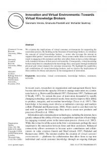
locomotion system is presented in Figure 2. From this figure, it can be seen that our motion control mechanism is hierarchical in nature.

Locomotion parameters (Path generation) high-level control

State-phase timings

Environment information

Locomotion strategies

Footprint planning

Updated swing foot trajectory Yes

Updated pelvis trajectory

Collision detected ? No No

middle-level control

Stance foot trajectory

Inverse kinematic Optimization ?

Stance leg kinematics

Pelvis (root) trajectory

Swing foot trajectory

Yes

Swing leg kinematics

3. General Overview 3.1 Human Model Representation

Locomotion attributes

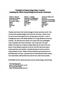
The articulated figure we use to simulate human walking were constructed from rigid links connected by rotary joints of up to three degrees of freedom. The model that we use for the examples in this paper has 18 joints with total of 36 degrees of freedom, excluding the hands, as shown in figure 1. y

Upper body kinemnatics

Lower body kinematics

Gait determinants

low-level control

Motion modules

Body joint angles

Figure 2. Locomotion system structure.

4. Motion Control at the High Level

y

x x y

z

neck-3d

chest-1d, X

z

y x

shoulder-3d z y

waist-3d

x

elbow-1d, X

y

z

x y

x z

hip-3d

z

y

wrist-2d, X,Z x

knee-1d, X

x

z

pelvis-3d

y

4.1 Locomotion Parameters

z x

y

ankle-2d, X, Z

z

x z

y

Motion control at the high level allows the user to animate the motions with a small number of locomotion parameters. Given the traveling path and desired speed, the system will compute the 3D path information and its corresponding locomotion strategies to generate walking motion automatically.

b_foot-1d, X x

z

Figure 1: The controlled degrees of freedom of the human model. There are 18 body segments and a total of 36 controlled degrees of freedom.

3.2 Locomotion System Structure In our system, goal-directed inverse kinematics, incorporated with optimizations of limb trajectories and joint angles, are used in computing the motions of human walking in virtual environments. The basic structure of our

Finding a safe path from a starting location to a destination in an arbitrary environment represents a challenging task in several research fields. In the real world, when an obstacle is encountered in the path, we have two options: go around it by changing the walking direction, or go over it by modifying limb trajectories. For example, if the obstacle is too big to go over, the walker has to alter his walking direction to go around it. Research fields, such as robotics and artificial intelligence, have provided rich sources to solve this path-searching problem; however, this is beyond the scope of this paper. At the writing of this paper, our system lets the user design the global path on the horizontal plane by specifying the piecewise cubic polynomial curves and their control points. Walking speed serves as one of the most important factors in determining gait characteristics. Using the speed

parameter and human height, important gait determinants, such as step length and step frequency, can be automatically generated. A good example from Bruderlin and Calvert’s work [4] shows the relationship between velocity and step length in normal walking as Step length = √ 0.004 × S × body_height (1) S (m / min) = Step length × Step frequency (2) Where S is the speed of the torso; Step length: the distance between successive foot-floor contact with opposite feet; Step frequency: steps being taken in a given time. For the purpose of various gait motions, the user can overwrite these attributes arbitrarily. For example, in certain steps during the locomotion, we may extend (shorten) the step length to overcome (or avoid) obstacles along the traveling path.

4.2 Step Planning and Locomotion Strategies Human locomotion studies [34, 39] have showed that foot placement is a precise control task and will help gait stabilization. To ensure correct and natural foot placement, planning the footprints at the right places along the global route is critical. Our approach arranges the footprints as a function of step length, direction change of the global route, and terrain status. On a flat, obstacle-free ground, a simple way to arrange the next footprint is to advance the current footprint location by the step length computed from equation (1) along the advance direction. However, an intelligent footprint planning mechanism with flexible step length is necessary for locomotion in an uneven terrain environment. Based on this consideration, the non-uniform step length for each step is computed as a function of direction change along the path, terrain status, and our locomotion strategies. Direction change Global route is the 2D body trajectory over the ground plane. First, a gross footprint planning algorithm with uniform step length is applied to place the estimated footprints along the path. The orientations of these estimated footprints are calculated as the tangent vectors along the path at footprint locations. If the directionchange exceeds a pre-defined threshold, the step length is reduced as a function of direction-change magnitude, whereas the step duration is unchanged. The decrease in step length for the same step duration during direction change indicates that the average speed of progression is reduced, thus allowing for a safe adaptation of locomotion patterns during advance direction change.

Terrain status Since the global path is specified in the 2D horizontal plane, it is necessary to map the path onto the world coordinate of the environment and get the 3D environment information along the path. Thus, we can apply our locomotion strategies to plan the footprints along the global path, determine supporting-foot trajectory, and search for a collision-free trajectory of the swing leg for each gait. Locomotion strategies Step length adjustment represents the most important type of gait adaptation while traversing in an uneven or cluttered environment. Experimental data show that location of the obstacle has no effect on human’s ability to go over the obstacle safely when the reaction time is given at least two-step duration ahead [23]. Using this observation, with linear interpolation of step lengths among consecutive steps, our footprint planning mechanism plans the footprints two steps ahead, and computes the step length of current step, based on step lengths of previous, current (estimated), and next (estimated) steps. This intuitive, yet simple, footsteps planning scheme works reasonably well in variant terrain as “readiness” for next step is prepared by including the estimated step length of next step, while “continuity” between consecutive steps is achieved by including both the previous step length and the estimated current step length.

5. Motion Control at the Middle Level At the middle level of control, attributes regarding the lower body, such as the weighting factor of leg joints, are provided to allow the user to produce a variety of gait characteristics.

5.1 Stance Foot Trajectory Stance foot trajectory represents one of the end-effector trajectories in our inverse kinematic mechanism. The support phase starts after the heel strikes the ground. Then, after a small fraction of support duration, the foot stays flat on the ground for most of the duration, follows by pushing off the ground at the end of support phase. Since foot state-phase timing is given as is footprint location, the trajectory of the stance foot can be determined by two parameters: the place-on angle (between the foot and the ground) at the beginning of the support phase, and the liftoff angle at the end of the support phase (Figure 3). Results in gait observation [37] have shown that the ankle joint is generally close to its neutral angle in plantarflexion/dorsiflexion at the times of foot lift-off and initial contact. This angle is usually referred to as 90.

hip1

hip2

θ0 LL knee1

0.5π

0.5 π

θ1

θ2

θ’1

knee2

0.5 π

0.5π

LL = Leg Length 0.5 x SL

θ’2

SL = Step Length

0.5 x SL

(a)

(b)

Figure 3. Two- stage process for computation of the foot place-on and lift-off angles. (a). Symmetric compass gait is assumed and used to compute the estimated foot place-on and lift-off angles between the foot and ground (θ0 = θ1 = θ2). (b). Based on θ0, gross pelvis position at middle of double support phase is found and used to compute the refined θ’1 and θ’2. Research in gait mechanics [29] also suggests that the configuration of the supporting leg (θ0 hip flexion, full knee extension, and ankle at neutral) at the beginning of supporting phase provides optimum balance between step length and stable weight loading. Applying this theory to our computation of the place-on and lift-off angle parameters, we assume the ankle joint is at its natural rest configuration (as an alternative, it can be arbitrarily adjusted by the user.) when the foot starts to place-on the ground for weight bearing, and lift-off from the ground for leg swinging. First, symmetry compass gait is assumed and used in the computation of the preliminary foot place-on (θ1) and foot lift-off (θ2) angles. Using these preliminary angles, incorporated with our pelvis-trajectory defining algorithm (described in later section), the gross pelvis position at the middle of double support phase is found. Then, inverse kinematics takes the pelvis and ankle positions to compute the hip and knee joint angles. Finally, the angles at foot place-on (θ′1) and lift-off (θ′2) are computed by adding their respective hip and knee joints. Once the two parameters, foot at place-on and lift-off angles, are determined, defining the trajectory of the stance foot is a relatively straightforward task. Linear interpolation is used in the time intervals from foot placeon to flat foot, and from flat foot to foot lift-off, to compute the angle between the support foot and ground. Knowing this angle parameter at given times with footprint’s location, the trajectory of the stance foot is defined.

5.2 Pelvis Trajectory during the Gait Cycle After the stance foot trajectory is defined, one of the endeffector trajectories is given. Next, we need to find out the root (pelvis) trajectory for inverse kinematics to work. However, finding the pelvis (or root, in kinematics mechanism) trajectory is a non-trivial task for animating human locomotion.

Previous work such as Girard [12] used sinusoidal interpolation between an arc-like curve, which shows the knee joint stiffness during mid-stance phase, and a piecewise speed curve to simulate the pelvis trajectory during the stance phase. Bruderlin and Calvert [4] used a simplified dynamic model and control algorithm to animate human walking. Step symmetry based on compass gait was assumed, and a length-changing telescopic leg with two degrees of freedom, simulating the stance phase, was used to compute the pelvis trajectory. Both Girard and Bruderlin’s approaches work reasonably well in modeling pelvis movement of the human normal walking gait. However, for simulation of human walking on uneven terrain, their approaches appear insufficient to generate the desired pelvis trajectory. Human gait observation has shown that the shape of the human pelvis trajectory in walking is similar to a smooth sinusoidal curve as shown in figure 4.

y

a

c

z

b

x

Figure 4. Displacements of pelvis in three planes of space. a. Lateral displacement in horizontal plane; b. Vertical displacement in a sagittal plane; c. a and b are projected and combined to form c as the 3D pelvis trajectory.

On the sagittal plane (projection of the 3D curve onto the YZ plane.), the pelvis reaches the summits at about the middle of the stance phase, and falls to the bottoms during the middle of the double support interval, when both feet are in contact with the ground. From geometric point of view, cubic splines should be able to define the shape of the pelvis trajectory curve with minimal control points. Thus, based on the following considerations, we chose Bezier curve to model the pelvis trajectory of human walking: •

The two end points which the Bezier curve will pass through are well suited to represent the vertical maximum and minimum of the sinusoidal pelvis curve.

•

• •

First-order continuity between adjacent segments is achieved by imposing the constraint that the third control point from previous segment and the second control point from the current segment are to be collinear. Due to pelvis’s local activity, varied horizontal velocities of the pelvis during the gait cycle can be simulated by adjusting the in-between control points. It is easy to reshape the Bezier curve by adjusting one or two control points, and the computational requirements are reasonable.

Using the Bezier curves to represent the geometry shape of pelvis motion curve during locomotion, we have to position the control points properly, and then define how the pelvis moves along the curve. Summit at mid-stance The pelvis passes through its vertical maximum at the middle of leg supporting duration, also known as midstance (MS). Since the supporting foot stays flat on the ground at this moment, knee joint flexion is the deciding factor to compute the location of the pelvis at mid-stance. Thus, given a highly-extended knee joint, the vertical displacement will then be enlarged, and results in a bouncy gait. On the contrary, large flexion of the knee joint reduces the magnitude of the vertical displacement of the pelvis trajectory, and generates a smoother pelvis curve.

2.

3.

energy consumed, which plays an important criteria in human locomotion. Given configurations of end-effectors, inverse kinematic computes each joint angle of the articulated chain automatically. Candidate curves which tend to produce jerky joint motion in consecutive frames are unfavor to equation (3) and will be eliminated. Using weighting factor for each joint gives the animator the flexibility to animate a variety of walking styles.

For the supporting leg, since the foot (end-effector) trajectory is known, given the pelvis (root) trajectory during supporting phase, inverse kinematics is applied to compute the in-between joint angles of the supporting leg during stance phase. In the objective function, the weighting factors define the relative importance and contribution of a given joint. Coefficients from leg jointstiffness observed in a gait lab are normalized and applied as the default weighting factors in the objective function. As an alternative, the user can arbitrarily adjust these weighting factors to generate various gait characteristics.

Pelvis at mid-stance Pelvis at middle of double support pt3

pt2 pt1

Valley at middle of double support The pelvis passes through its vertical minimum at the middle of the double support phase (MDS). The timing of the MDS is right in the middle of two consecutive MSs, but the pelvis location at MDS could be anywhere inbetween the two MSs as shown in figure 5. Since each possible location of the pelvis at MDS will define a different motion curve for the pelvis, given the pelvis location at MDS, we use an optimal approach, which tries to minimize the sum of angular accelerations of supporting leg joints during supporting phase, to evaluate the resulting curve: ∇[

i=3

∑ Wi ∫ i=1

xmid _sup port

xstart _sup port

j=3

f i ( x)d 2 x +

∑ j=1

Wj

∫

xend _sup port

xmid _sup port

f j ( x )d 2 x ]

where Wi is the weighting factor of joint i; fi (x) is the ith joint angle computed from kinematic algorithm at time x.

A

Figure 5. Pelvis location at consecutive MSs. The optimal objective function is used to evaluate each of the 5x5 grid area. Then, the qualified cell is further subdivided into another 5x5 grid, and evaluation is applied again to find the best pelvis location at MDS.

(3)

inverse

The reasons behind using equation (3) as our optimization function for evaluating the candidate motion curves are: 1.

A2,3

Supporting leg is the major limb that moves forward and balances the whole body during locomotion. Minimizing the sum of supporting leg joint angular accelerations, in general, means minimizing the

As shown in figure 5, the pelvis location at MDS (pt2) is somewhere in area A between pelvis locations at MSs (pt1 and pt3). First, area A is subdivided into a 5x5 grid. The centroid of each cell is then used to form a curve to be evaluated by our objective function (equation 3). Then, the grid with the best-scored curve is subdivided into another 5x5 grid. Like the previous process, each centroid of the new subdivided grid is used to form a curve to be evaluated by the same objective function. The best-scored centroid of the second-level grid is then selected to be the pelvis location at MDS, and forms the pelvis (root) curve in our inverse kinematic mechanism animation. By using

this two-level subdividing approach, area A is subdivided into 625 sub-areas. Therefore, instead of evaluating all 625 curves, less than 1/12 of them (most of them can be eliminated at a very early stage of evaluation, due to out of working space of the articulated chain.) are actually evaluated to find the most satisfying curve. The algorithm to search for the pelvis location at MDS works as follows: at each level of subdividing // 2 levels, each is a 5x5 grid for ( i=1; i ≤ 25; i ++) { build the pelvis curve; t = 0; while ( t ≤ 1.0) { t = t + ∆t; find pelvis and heel locations at t; inverse kinematics to get in-between joint angles; score(i) = score(i) + equation (3); } if ( score(i) < min_score ) min_score = score(i); } return (i); Pelvis movement along the curve trajectory Despite the geometrical shape of the pelvis trajectory, the Bezier curve itself doesn’t provide much information about pelvis’s movement along the curve. Thus, further regulation of this curve is required to improve the walking model. Throughout the gait cycle, pelvis moves forward with little variance in speed, being fastest during the double support phase and slowest in the middle of the stance phase [37]. From the captured motion data we collected, we found that “pelvis” moves in such a pattern not only in normal gait, but also in stair-climbing, descending, and obstacle-overcome gaits (appendix A). These observations indicate there is a generic displacement vs. time pattern of pelvis motion for all gaits. To simulate the same pattern of pelvis movement during the gait cycle, a non-uniform time-space sampling approach is applied to the Bezier curve. The parameter t of the Bezier curve is computed as:

t

new

=

∫

t s a m p l in g

0

f (t )dt ∫ f (t )dt

(4)

1

0

that ends at t = tsampling. Thus, the parameter t of the Bezier curve is adjusted and normalized by the motion-captured data.

5.3 Swing-leg trajectory during the gait cycle The swing-leg trajectory represents another end-effector trajectory. Bezier curve, with same advantages as for defining the pelvis trajectory, is again applied to represent the desired trajectory of the swing foot. Since the root trajectory has already been determined, the main concerns in defining the trajectory of the swing leg include: Collision avoidance During the normal swing phase, the leg that is not in contact with the ground should clear the ground by a reasonable and safe margin. If there is an obstacle presented in the path of the swing leg, the priority is clearly to provide adequate elevation of the foot, depending on the location of the obstacle and the body posture at that time frame. For collision detection, the positions of the toe and heel are examined against the ground surface. Least energy spent Foot trajectories have been investigated in relation to energy expenditure [17, 28]. In general, trajectories tend to be chosen to minimize energy spent, which explains the low small toe clearance during normal gait. In an uneven terrain environment, if a surface obstacle is presented in the path of the swing leg, the most important factors we need to be concerned of are obstacle height and location, which reflect the unevenness of the terrain that is commonly encountered. A Bezier curve, which maintains a low safe margin above the terrain surface, is applied to represent the trajectory of the swing leg. The ankle of the swing leg at lift-off and place-on, which we have computed in stance foot trajectory section, are set to be the starting and ending points of the Bezier curve, and the inbetween control points of the curve are elevated from the ground until the whole curve safely passes above the surface without collision (Figure 6). Not surprisingly, our results show that the Bezier curve defined by maintaining a small margin over the obstacles also satisfies equation 3. We think the possible reasons behind this are: •

where f(t) is the “generic” motion-captured pelvis trajectory during the gait cycle. Setting the parameter t’s

∫ f (t )dt is the whole pelvis trajectory, 1

range from 0 to 1, while

∫

tsampling

0

0

f (t )dt represents the piece of the trajectory

•

Maintaining minimal toe clearance while keeping collision-free, in general, produces a “flat” Bezier curve. Also, the “smoothness” characteristic of Bezier curves results in the smoothness of joint-angle movement. Raising the leg more than what is necessary, from inverse kinematic point of view, causes more flexion in the hip and knee joints, which is unfavorable to our

optimization function (equation 3). Experimental data from gait observation also shows that raising the leg entails an additional energy cost.

P1 and P 2 are elevated from the ground until a collision-free Bezier curve is formed

P3

P2

P1

Po and P 3 are the ankle positions at foot place-on and lift-off, which were computed in the stance foot trajectory section

motions without violating kinematic constraints, such as foot penetration or foot slippage on the ground, and obstacle collision. Among these adjustable animating attributes, gait determinants are the most important ones regarding locomotion.

6.1 Gait Determinants Gait determinants in our system include three activities of the pelvis during the gait cycle. They are pelvic rotation, pelvic tilt, and lateral pelvic displacement: •

P0

Figure 6. A Bezier curve to represent trajectory of the swing foot. Minimal toe clearance is maintained above upraised obstacle.

Coordinate synchronization Footprints were pre-planned based on step length and environment information. Therefore, coordinate in relation to the environment (world) is the natural choice of coordinate frame to define the trajectory of the swing foot in. The possible swing-foot trajectories are then defined to be starting from the foot lift-off of footprint n and terminating at the heel touchdown of footprint n+2, with the in-between control points to avoid obstacle collision and minimize energy. These curves are then mapped to the coordinate system with reference to the pelvis to make sure the foot (end-effector) is within the working space (where the base is at the pelvis), and finally, the curve with minimal sum of toe-clearance over the terrain surface is chosen to represent the swing foot trajectory. Foot movement along the swing-foot trajectory Just like pelvis’s movement in gait cycle, the swing foot also moves in a quite “generic” displacement vs. time pattern (appendix B) in various gaits. The speed generally varies a little during swing phase, being fastest during the middle and slowest in the beginning and terminating of the swing phase. Thus, equation 4 is applied again for adding “dynamic” into the swing-foot trajectory.

6. Motion Control at the Low Level One of the advantages of our motion control mechanism is that it allows the user to fine-tune the appearance of the motion at the final stage of animating. At this stage, since the major joint configurations of the legs are known, as is the root configuration of the articulated body structure, it is possible to tune-in the other attributes to achieve desired

•

•

Pelvic rotation: pelvis rotates about the body trunk alternatively to the left and to the right, relative to the walking direction. As an index for animating, Saunders et al. [15] quote ± 3° for the amplitude in normal walking gait. Pelvic tilt: in normal walking gait, due to pelvis tilt ( ± 5° about the walking direction axis), the hip of the swing leg falls slightly below the hip of the support leg. Introducing pelvis tilt needs to be carefully implemented because it can jeopardize the possibility of the swing foot penetrating the ground surface. To compensate this undesired effect, a more knee flexion of the swing leg is necessary. Lateral pelvic displacement: normal walking involves displacement of the pelvis from side to side. For each stride, the maximal lateral displacement (to the support side) happens during the middle of support phase at an amplitude of approximately 4 to 5 cm.

6.2 Personalized Human Locomotion Although the focus of this paper is to provide an animation scheme with regard to leg motions of human walking in virtual environments, a variety of walks with different personalities and moods can still be obtained by modifying the basic motion generated from algorithms. Currently, our system, at the lowest control level, allow the user to animate various walks through the following approaches: Adjusting control parameters Controlling parameters are the desired angle and position for the joints of the animated human figure. At the lowest control level, the user can easily adjust the control parameters, except for those system-lock parameters generated from algorithms, and watch the result motion immediately. Various walks can be animated by tweaking one or multiple of the control parameters. For example, the support knee joint angle at mid-stance will affect bounceness of the walk, while lateral displacement of the pelvis during the support phase can be adjusted to simulate walks of different sexes; with the default lateral displacement value, if we scale up the value, the human

figure walks more like a woman. On the contrary, scaling down the value will make the figure’s walk more man-like and robotic. Giving another example, some parameters can be tweaked around to simulate certain walking styles; a “proud” or “happy” walk can be obtained by adjusting arm swing and shoulder rotation to their maximum, while torso and head tilt to their minimal. On the other hand, a “tired” or “frustrated” walk is achieved by tweaking the same parameters in opposite direction. Overwriting with motion modules Another way to add variety to walk motions is to overwrite the basic motion with motion modules. A motion module is a motion sequence of a sub-set of the bodies. Typically motion modules are pre-processed animation sequences from algorithms or motion capturing. Based on the functionality of the module, we divide the human model into five sub-sets of the bodies; upper body (trunk and head), left arm, right arm, left leg, and right leg. Considering applying motion modules as a post-processing task of the basic motion, flexibility is given to the user to pick desired motion modules, plug in, and play them.

7. Results We have successfully applied our algorithms for animating human walking. The advantages of our approach over the other human locomotion systems are: Functionality Besides normal walking, our approaches are capable of animating human walking on uneven terrain. Smooth motions of the lower extremities are ensured by the objective function which attempts to minimize joint-angle differences between consecutive time frames through gait duration, while foot placement and trajectory are precisely controlled to prevent negative animation artifacts, such as the stance-foot sliding during the support phase and collision with obstacles. Figure 7 illustrates sequences of walking with various gaits in different environments. Flexibility Through the hierarchical motion control mechanism, the desired motions can be flexibly directed and controlled. At the high level, only some minimal locomotion parameters, such as “destination” and “speed” are required to generate the correspond basic motions. While at the middle level, additional locomotion parameters, such as state-phase and gait determinants, are used to achieve different gait characteristics. Finally, at the low level, pre-processed motion modules are plugged in, or animation attributes regarding the upper body are fine-tuned, to animate various locomotion styles and personalities,

Runtime complexity The major computation in our algorithms is defining the pelvis trajectory through the gait cycle. A subdividing-inlevel approach is applied to minimize the number of possible curves that the objective function has to evaluate. For example, among the nm possible curves, m × n curves are actually evaluated, where n is the number of uniform cells, and m is the number of levels. This scheme with relatively cheap inverse kinematics is used in computing the joint angles of the lower extremities. Thus real-time simulation can be easily achieved. We have implemented our control algorithms on a Pentium-II 300 MHz (with 128M RAM) PC, and successfully computed an average of 3.75 steps (10 frames/step) motion for each second. The results also indicate the computational complexity is terrain-independent, that is, complexity of the terrain has virtually no impact on the system’s performance. Considering that normal human step frequency is only about 1.8 steps per second, our motion control mechanism can be used to simulate real-time motion easily and let the precious computing source devote to other tasks.

8. Conclusions A hierarchical motion control mechanism has been introduced which allows the animator to generate a variety of real-time human walking in virtual environments. Motion control at the top level allows the user to animate basic locomotion by specifying minimal-required parameters; the traveling path and locomotion speed. The path is generated based on the piecewise cubic polynomial curves and their control points so that its shape can be easily adjusted to avoid obstacles, while the walking speed is used to determine the gait characteristics. This provides the user a simple way to animate desired walking motion by giving command, such as “walk this route at speed X”. Like most human animation systems, the major problem in animating human locomotion is to define the limb trajectories, especially the root (usually the pelvis or the supporting limb) trajectory. The computations of the limb trajectories in our system are based on observations of human walking given by motions captured, and our “energy optimization” approach. Using this technique incorporating with human gait behaviors observed in experiments, such as foot placement strategies, natural human walking within an obstacleridden environment can be successfully simulated in real time. At the lowest level of controlling, further varied motions can be added by the user by adjusting animation parameters, such as joint angles, or plugging in preprocessed motion modules, such as captured motion sequences. At this level, a satisfying motion is already

generated by the system. For a desired motion, all the user has to do is overwriting the basic motion by modifying necessary parameters, or with motion modules. Because of the simplicity of overwriting the existing motion, a variety of walks can be created interactively and in real time. As our initial step of building a system that is capable of simulating human locomotion in a variety of virtual environments, our current system still has a lot of explorations and improvements to do. For example, the controlling criteria to affect the motions of the lower body include the cubic polynomial and the weighting factors of the objective function; changing the curve or altering the weighting factors certainly will give a different walking behavior. A possible improvement of our system is to build the interactive relationship between these parameters and a variety of walks (personality, or mode), so the user can animate the desired motion by giving commands, such as “happily walks from A to B with speed X.”, instead of determining these parameters by trial and error. Finally, we believe our system can be greatly improved if we manage to integrate knowledge from various research fields, such as artificial intelligence and human psychology (for path and footprints planning), biomechanics, and human gait observation (motion capturing).

a. Leg motion in normal walking gait.

b. Walking sequence on uneven terrain. Left leg in motion.

c. Same walking sequence as b. Right leg in motion.

Figure 7. Walking sequences on different environments

Appendix A: The displacement vs. time patterns of pelvis movement in various gaits

References 1.

The speed of pelvis varies a little as it moves forward during leg-supporting phase, being slowest in the middle of leg-supporting phase and fastest during the double support phase. The following charts show the displacement vs. time patterns of pelvis movement in various gaits (level, descending, and ascending). All three charts have a quite similar displacement vs. time pattern, thus, we conclude a “generic” displacement vs. time pattern can be form to represent pelvis movement for all gaits.

2.

3.

4.

5. D (cm)

D (cm)

D (cm)

100

100

100

50

50

50

T 50 %

6. 7.

T

100 %

50 %

T

100 %

50 %

Descending

Level

Height diff. : 20 cm

Step length: 60 cm

D: displacement

100 %

8.

Ascending Height diff. : 20 cm

T: support phase

9. 10.

Appendix B: The displacement vs. time patterns of foot movement in various gaits The speed of swing-foot varies during swing phase, generally being fastest during the middle and slowest in the beginning and terminating of the swing phase. The following charts show the displacement vs. time patterns of pelvis movement in various gaits (level, descending, and ascending). Just like the pelvis’s motion pattern, a “generic” displacement vs. time pattern can be form to represent pelvis movement for all gaits.

D (cm)

D (cm) 150

150

100

100

100

50

50

50

T 50 %

100 %

100 %

14.

17. T 50 %

Level

Descending

Ascending

Step length: 60 cm

Height diff. : 20 cm

Height diff. : 20 cm

D: displacement

13.

16.

T 50 %

12.

15.

D (cm)

150

11.

100 %

18.

T: swing phase

19.

Note: Data of appendix A and B are collected from our motion capturing work at National Institutes of Health.

W. W. Armstrong, and M. W. Green. 1985. “The Dynamics of Articulated Rigid Bodies for Purposes of Animation.” The Visual Computer 1(4): 231-240. T. Andriacchi, G. Anderson, R. Fermier, D. Stern, and J. Galanta. 1980. “A Study of Lower-Limb Mechanics during Stair-Climbing.” J. Bone and Joint Surgery. 62A, pp. 749757. R. Boulic, N.M. Thalmann, and D. Thalmann. “A Global Human Walking Model with Real-time Kinematic Personification.” The Visual computer, 1990, 6, 344-358. A. Bruderlin and T. W. Calvert. 1989. “Goal-Directed Dynamic Animation of Human Walking.” Computer Graphics 23: 233-242. A. Bruderlin and T. W. Calvert. 1993. “Interactive Animation of Personalized Human Locomotion.” Graphics Interface 1993, pp. 17-23. A. Bruderlin and L. William. 1995. “Motion Signal Procession.” Computer Graphics 29(4): 97-104. A. Bruderlin and T. W. Calvert. 1996. “Knowledge-Driven, Interactive Animation of Human Running.” Graphics Interface 1996, pp. 213-221. Cappozzo and T. Leo. 1974. “Biomechanics of Walking up Stairs.” 1st CISM-IFTOMM Symp. on Theory and Practice of Robots and Manipulators., pp. 115-132. R. Featherstone. 1988. Robot Dynamics Algorithms. Kluwer Academic Publishers, Norwell, MA. J. Flynn. 1977 “Kinematical Variability of Normal Climbing and Descending Stairs.” M. Sc. Thesis, Vanderbilt University, Nashville, TN. M. Girard and A. A. Maciejewski. 1985. “Computational Modeling for the Computer Animation of Legged Figured.” Computer Graphics 19(3): 263-270. M. Girald. 1987. “Interactive Design of 3D ComputerAnimated Legged Animal Motion.” IEEE Computer Graphics and Applications 7(6): 39-51. L. Gritz and J. Hahn. 1995. “Genetic Programming for Articulated Figure Motion.” J. of Visualization and Computer Animation, vol. 6: 129-142. M. Gleicher. “Motion Edition with Spacetime Constraints.” Proc. 1997 Symposium on Interactive 3D Graphics. Apr. 1997, pp. 139-148. M. Gleicher. 1998. “Retargetting Motion to New Characters.” Computer Graphics, 32(4): 33-42. J. K. Hodgins, W.L. Wooten, A.C Brogan and J.F. O’Brien. 1995. “Animating Human Athletics.” Computer Graphics, 29(4): 71-78. K. G. Holt, J. Hamill, and R. O. Andres. 1991. “Predicting the minimal energy costs of human walking.” Med. Sci. Sports Exerc. 23, pp. 491-498. H. Ko and N. I. Badler. 1993. “Straight-line Walking Animation based on Kinematic Generalization that Perserves the Original Characteristics.” Graphics Interface ‘93, pp. 9-16. H. Ko and N. I. Badler. 1996. “Animating Human Locomotion with Inverse Dynamics.” IEEE Computer Graphics and Applications, Mar. 1996, pp. 50-59.

20. L. Livingston. 1984. “Kinematic Analysis of Stair Climbing.” M. Sc. Thesis. Queen’s University, Kingston, Ontario. 21. B. J. McFadyen and D. A. Winter. 1988. “An Integrated Biomechanical Analysis of Normal Atair Ascent and Descent.” J. Biomechanics, 21(9), pp. 733-744. 22. M. McKenna and D. Zeltzer. 1990. “Dynamic Simulation of Autonomous Legged Locomotion.” Computer Graphics 22(4): 29-38. 23. A. E. Patla, S. D. Prentice, C. Robinson, and J. Neufeld. 1991. “Visual Control of Locomotion: Strategies for Changing Direction and for Going over Obstacles.” J. Exp. Psychol. Human Percep. Perform. 17, 603-634. 24. K. Perlin. “Real-Time Responsive Animation with Personality.” IEEE Trans. on Visualization and Computer Graphics, Vol. 1, Mar. 1995, pp. 5-15. 25. J. Perry. Gait Analysis. McGraw-Hill, New York. 1992. 26. C. B. Phillips and N. I. Badler. 1991. “Interactive Behaviors for Bipedal Articulated Figures.” Computer Graphics 25(4): 359-362. 27. M. H. Raibert and J. K. Hodgins. 1991. “Animation of Dynamic Legged Locomotion.” Computer Graphics, 25(4): 349-358. 28. M. S. Redfern and T. Schumann. 1994. “A Model of Foot Placement during Gait.” J. Biomechanics, 27(11): 13391346. 29. C. F. Rose, B. Guenter, B. Bodenheimer, and M. F. Cohen. 1996. “Efficient Generation of Motion Transition Using Spacetime Constraints.” Computer Graphics 30(4): 147154. 30. C. F. Rose, M. F. Cohen, and B. Bodenheimer. 1998. “Verbs and Adverbs: Multidimensional Motion Interpolation.” IEEE Computer Graphics and Applications, Sept. 1998, pp. 32-40. 31. K. Sims. 1994. “Evolving Virtual Creatures.” Computer Graphics 25(4): 15-22. 32. D. Sturman. “Interactive Keyframing Animation of 3-D Articulated Models.” Graphics Interface ‘86, Tutorial on Computer Animation, 1986. 33. N. M. Thalmann, and D. Thalmann. Computer Animation: Theory and Practice. Springer-Verlag, New York, 1990. 34. A. Townsend. 1985. “Biped Gait Stabilization via Foot Placement.” J. Biomechanics Vol. 18. No. 1. pp.21-38. 35. M. Unuma, K. Anjyo, and R. Tekeuchi. 1995. “Fourier Principles for Emotion-Based Human Figure Animation.” Computer Graphics 29(4): 91-96. 36. M. van de Panne, 1997. “From Footprints to Animation.” Computer Graphics Forum, 16(4): 211-223. 37. W. Whittle. Gait Analysis: an introduction. ButterworthHeinemann, Oxford. 1996. 38. J. Wiley and J. K. Hahn. “Interpolation Synthesis for Articulated Figure Motion.” Proc. Virtual Reality Annual Int’l Symp., IEEE CS Press, Mar. 1997, pp. 156-160. 39. A. Winter. 1992. “Foot Trajectories in Human Gait: a Precise and Multifactorial Motor Control Task.” Phys. Therapy 72(1): 45-53. 40. A. Witkin and M. Kass. 1988. “Spacetime Constraints.” Computer Graphics 22(4): 159-168. 41. A. Witkin and Z. Popovic. 1995. “Motion Warping.” Computer Graphics 29(4): 105-108.

42. D. Zelter. 1982. “Motor Control Techniques for Figure Animation.” IEEE Computer Graphics and Applications, 2(9): 53-59.