Anomaly detection of notebook computer based on Weibull decision metrics Gang Niua, Satnam Singhb, Steven W. Hollandc, Michael Pechtad a
Center for Prognostics and System Health Management, City University of Hong Kong, 83 Tat Chee Avenue, Kowloon, Hong Kong
[email protected] b Diagnosis and Prognosis Group, GM India Science Lab, GM Global R&D, Bangalore, India
[email protected] c Electrical & Controls Integration Lab, GM Global R&D, Warren, Michigan 49090, USA
[email protected] d Center for Advanced Life Cycle Engineering (CALCE), University of Maryland, College Park, Maryland 20742, USA
[email protected]
Abstract – This paper presents a novel approach for health monitoring of electronic products using the Mahalanobis Distance (MD) and Weibull distribution. The MD value is used as a health index, which has the advantage of both summarizing the multivariate operating parameters and reducing the data set into a univariate distance index. The Weibull distribution is used to determine health decision metrics, which are useful in characterizing distributions of MD values. Furthermore, a case study of notebook computer health monitoring system is carried out. The experimental results show that the proposed method is valuable. I. INTRODUCTION With the rapid advancements in industry and growing business competition, electronic products require enhanced safety and reliability so as to reduce their vulnerability to serious failure and the failure of host systems. The reliability of a product is defined as the ability of that product to perform as intended (i.e., without failure and within specified performance limits) for a specified time in its life cycle application environment [1]. As a product begins to undergo stresses and begins to have its useful life consumed, its current condition is subject to change due to those stresses. Some changes in the operation can be classified as “abnormal” since the system is behaving in a manner that is outside specified performance limits. Product health monitoring is one such strategy that evaluates a product’s health during operation by measuring and recording the extent of deviation and degradation from the product normal operating states. Benefits of health monitoring can reaped in terms of advance warning of failure, prevent catastrophic failure, assess reliability, reduce unscheduled maintenance, identify faults efficiently, and improve both qualification methods and the design of future products [2]. Electronic products are manufactured by integrating several sub-assemblies, components, and parts that can fail due to various failure mechanisms in the product’s life-cycle environment. The anomalous behavior of an electronic product often prompts a customer to return the product to a retailer or a
manufacturer. At a retailer’s facility or at manufacturer’s site the product often goes through extensive tests. In many cases, these tests fail to reproduce the exact anomalies or faults and hence the discovery of the root cause behind the anomalous behavior is difficult [2]. Ability to detect anomalous behavior during the product’s operation can help in freeing some resources invested in post failure analysis and identifying the root cause behind failure events. Kumar et al. has presented an approach to utilize MD value for the continuous health monitoring through control chart, where MD values are transformed into Gaussian form [3]. In this paper, we discuss a novel health monitoring method using Mahalanobis distance (MD) index and Weibull decision metrics as shown in Fig.1. Before implementing any health monitoring strategies it is important to identify relevant parameters that should be measured [4]. First, the failure modes, mechanisms and effects analysis (FMMEA) of a product is carried out to select specific performance parameters, which can characterize the state of product’s health. Then we employ data relating to the selected performance parameters from healthy products to compute baseline statistics. Data preprocessing using normalization is conducted on the collected healthy data. Next, we compute MD values of the multivariate health data to summarize the data and then, a Weibull distribution is fitted on the healthy MD values. Finally, the first, second and third metrics are calculated from the fitted Weibull distribution, which will be used as alarm thresholds to detect anomalies in the product's health. The MD for health monitoring has the advantages of reducing a multivariate data set into a univariate distance index, which is sensitive to inter-variable changes in system health. The Weibull distribution is able to take on different shapes and is useful in characterizing distributions of MD values, which are not always of a Gaussian nature. The rest of this paper is organized as follows. In Section II, the proposed system is introduced, and the basic knowledge of each part in this system is explained in detail. Section III describes a notebook health monitoring experiment to demonstrate the effects of this system; the experimental results are also discussed. At last, conclusions and future work is described in Section IV.
Fig. 1 Health Monitoring System II. MD-Weibull Health Monitoring System To compare with other distance-based monitoring systems, the stated characteristics of this approach are use of determination of decision metrics. The use of distance-based metrics in determining the condition of a system or in identifying an “out-of-control” state is quite common and has been used successfully in different areas. A prime example of distance-based health metric is Shewhart control chart which uses the standard deviation and the mean of the distribution of “in-control” system values to detect anomalies. Here, we detect anomalies by computing the statistical dispersion of the test MD values with respect to the decision metrics. We first capture the correlations among health operating parameters by computing the MD values; then, decision metrics are computed by fitting Weibull 2-parameter distribution on the MD values. The Weibull 2-parameter distribution, when fit to the distribution of health MD data, provides a standard value, its mean. The mean of the Weibull 2-parameter distribution is:
µ = ηΓ 1 +
1 β
(1)
where η is scale parameter and β is shape parameter. From this, the location of each decision metric is determined. Drawing an analogy to the Gaussian distribution, we compute the decision metrics of the fitted Weibull distribution. It is known that the standard deviation, two times of standard deviation and three times of standard deviation roughly captures 66%, 95.7%, 99% of the Gaussian probability distribution.
Fig. 2 Proposed Method for Determining Weibull Decision Metrics Similarly, for the Weibull probability distribution, the region for which X% of the distribution occurs can be easily computed. For example, Fig. 2 illustrates the regions which capture the 68.27%, 95.45% and 99.73% of the probability distribution. With the metrics at hand, a standard—which can be used comparatively with test data to determine its system health—is made available. 2.1 Failure Modes, Mechanisms and Effects Analysis (FMMEA) The traditional Failure Mode and Effects Analysis (FMEA) methodology is a procedure to recognize and evaluate the potential failure modes of a product and their effects, and to identify actions that could eliminate or reduce the likelihood of
the potential failure to occur [5]. Many organizations within the electronics industry have employed or required the use of FMEA, but in general, this methodology has not generally proved satisfactory, except for the purpose of safety analysis [6]. A limitation of the FMEA procedure is that it does not identify the product failure mechanisms and models in the analysis and reporting process. Failure mechanisms and their related physical models are important for planning tests and screens to audit nominal design and manufacturing specifications, as well as the level of defects introduced by excessive variability in manufacturing and material parameters. Failure modes, mechanisms and effects analysis (FMMEA) methodology overcomes the weaknesses in the traditional FMEA process [6]. FMMEA is physics-of-failure (PoF) based methodology for assessing the root cause failure mechanisms of a given product [7]. A schematic diagram showing the steps in FMMEA is shown in Fig. 3. A potential failure mode is the manner in which a failure can occur—that is, the ways in which the item fails to perform its intended design function, or performs the function but fails to meet all of its objectives [89]. Failure modes are closely related to the functional and performance requirements of the product. Failure cause is defined as the process that initiates the failure and can help to identify the failure mechanism driving the failure mode. Failure mechanisms are the processes by which a specific combination of physical, electrical, chemical, and mechanical stresses induces failures. Failure effect is the effect that the failure has on the entire product or system. FMMEA prioritizes the failure mechanisms based on their occurrence and severity in order to provide guidelines for determining the major parameters that must either be at least accounted for in the design or controlled. A risk priority number (RPN) is calculated to represent the criticality of each failure mechanism. The RPN is the product of the occurrence and severity of each mechanism. Occurrence describes how frequently a failure mechanism is expected to result in failure. Severity describes the seriousness of the failure caused by such a mechanism. Define System and Identity Elements and Functions to Be Analyzed Identify Potential Failure Modes Identify Life Cycle Profile
Identify Potential Failure Causes Identify Failure Mechanisms Identify Failure Models Prioritize Failure Mechanisms Document the Process Fig. 3 FMMEA Methodology
FMMEA is based on understanding the relationships between product requirements and the physical characteristics of the product (and their variation in the production process), the interactions of product materials with loads (stresses at application conditions) and their influence on the product susceptibility to failure with respect to the use conditions. This involves finding the failure mechanisms and reliability models to assess the probability of failure. The process begins with gathering the information on product’s failure mechanisms, modes, environmental conditions, and performance parameters that can be monitored. Each monitored parameter is evaluated in terms of its ability to detect initiation of a failure mode. Parameters that can be identified for a given failure initiation are chosen for continuous monitoring. These enable decision and prognostic methods for a product’s health estimation and reliability monitoring. A failure precursor is an event or series of events that is indicative of an impending failure. For products with multiple usage conditions the precursor parameter must be selected such that a change in combined loading is accounted in the reasoning model.
2.2 Data Collection and Normalization Based on the determined precursor parameters using FMMEA and RPN, multivariate data are collected, and then a normalization process is exerted to the collected data. Here, normalization refers to the division of multiple sets of data by a common variable in order to negate that variable's effect on the data, thus allowing underlying characteristics of the data sets to be compared: this allows data on different scales to be compared, by bringing them to a common scale, which is a key step for performing the correct multivariate analysis. 2.3 Mahalanobis distance (MD) The MD methodology is a process of distinguishing multivariable data groups by a univariate distance measure that is defined by several performance parameters. The MD value is calculated using the normalized value of performance parameters and their correlation coefficients, which is the reason for MD’s sensitivity [10-11]. A data set formed by measuring the performance parameters of a healthy product is used as the training set for MD. The collection of MD values for a healthy system is known as the Mahalanobis Space. This is highly useful for health monitoring as MD can distinguish abnormalities from a “healthy” or “normal” group, and is essentially one main reason why MD is used in multivariate analysis [10]. The parameters collected from a system are denoted as Xi, where i = 1, 2,…, m. The observation of the ith parameter on the jth instance is denoted by xij, where i = 1, 2,…, m, and j = 1, 2,…, n. Here, m is the number of parameters, and n is the number of observations. Thus the (m × 1) data vectors for the healthy product are denoted by Xj, where j = 1, 2,…, n. Each individual parameter in each data vector is normalized by subtracting the mean ( X i ) of the parameter (Xi) and dividing it by the standard deviation (Si). These mean and standard
deviations are calculated from the healthy data. Thus, the normalized values are as follows: ( xij − X i ) zij = , i = 1, 2… m, j = 1, 2… n, (2) Si n
∑ (x
2 ij − X i ) 1 n j =1 where, X i = ∑ xij and Si = n j =1 (n − 1) Next, the values of the MDs are calculated for the healthy items using the following: 1 MD j = z Tj C −1 z j (3) m where zjT=[z1j,z2j,…,zmj] is a transpose vector of vector zj that comprises zij , and C is the covariance matrix calculated as:
C=
n 1 z j z Tj ∑ (n − 1) j =1
(4)
For fault detection, a threshold MD is defined using training (i.e., healthy) data. For a test system, the MD value is calculated for each observation by using the performance parameter’s mean, standard deviation, and a correlation coefficient matrix obtained from the training data.
2.4 The Weibull Decision Metrics based on Cumulative Distribution Function (CDF) The Weibull distribution is among the most important distributions used in reliability analysis [12]. One of the major strengths of the Weibull distribution is its ability to take on various forms by manipulation of its parameters. Using the Kolmogorov-Smirnov (K-S) Goodness-or-Fit test, we verify if the data follows the Weibull distribution. The 2-parameter Weibull distribution is defined as:
f (t ) = βη
−β
(t )
β −1
e
t − η
β
F (t ) = 1 − e
We want to compute x such that the area under the Weibull PDF between x and µ is X%. Therefore, we would like the difference in CDF value at the location where the mean occurs (which is known) and where the x location of the mean is to be X%. This method is explained graphically in Fig. 4 below. If it is desired to find x such that the area under the pdf to the left of µ and x is equal to X%, it would be expressed in the following way: F(μ) – F(x) = X%. Using probability theory, we obtain the x as follows: 1
β 1 x = η ln β µ − η e + X%
(7)
III. EXPERIMENT RESULTS AND DISCUSSION
( t ≥ 0, β > 0, η > 0 ) (5)
Where β is the shape parameter and determines the form of the graph while η is the scale parameter, which determines the spread of the distribution. The parameters (β and η) of the Weibull distribution can be estimated using maximum likelihood estimation (MLE) [13]. Because of the property of Weibull distribution to emulate other distributions, it is being used in order to provide a fitness for the distribution of health MD values. Then decision metric, which means a criterion of anomaly judgment, can be derived based on the distribution. The decision metrics are computed from the CDF of the Weibull distribution of health MD values. The CDF of the Weibull is defined as t − η
Fig. 4 CDF-based Decision Metrics
β
(6)
In this Section, an experiment of notebook computer health monitoring based on the proposed methods will be described. First, FMMEA was investigated to select effective performance parameters, and then a normalization process was performed on the collected dataset. Next, MD values of the healthy dataset were calculated. The calculated healthy MD distribution is utilized to fit Weibull parameters and determine the health decision metrics.
3.1 Identifying Health Monitoring Parameters In general, the phases of a life cycle profile include manufacturing, transportation, operation, and storage. A life cycle profile involves both environmental and operational loads that a system is exposed throughout its life. These loads may involve, for example, temperature, humidity, vibration, shock, power, or corrosion. It is important to understand a system’s life cycle profile to determine the actual loads that will affect the system’s performance and when those loads will occur. Additionally, information about the life cycle profile can be
used to eliminate failure modes that may not occur under the given application conditions. An FMMEA investigation was conducted on test notebook computers to determine better parameters, or failure precursors, which can be monitored for health detection. The selection of monitoring parameters is performed based on the most critical failure modes and mechanisms and their effects on system performance. The FMMEA was performed according to steps discussed in Fig. 3. Since there are many possible failure modes of a notebook computer, analysis is kept simple by considering only those failure modes that are observed at the system level. The results of the FMMEA indicate three high-risk failures within the notebook computers: • Rotation failures of the fan • Head crashes in the hard disk drive • Electrical shorts on the memory card Each of these failure modes is associated with one or more measurable variables, which should be monitored to indicate the occurrence of that failure in time. In this experiment, (i) temperature of the fan, hard disk drive and memory card, and (ii) memory usage capacity were selected as monitoring parameters.
3.2 Experiment Data Collection, Normalization and MD Calculation After performance parameters are determined, a total of 45 data patterns of healthy notebook computers (with same brand and type) were collected through sensors embedded on the fan, hard disk and memory card. Then data normalization was performed in order to eliminate the scale difference. Finally, MD values are calculated for each pattern, which translate multi-parameter into a single health index represented by the MD distance. The Histogram of the MD values is shown in Fig. 5. 3.3 Decision Metrics The shape and scale parameters were then extracted from the distribution and the mean of the distribution was calculated. The metrics were calculated in MATLAB and plotted against the healthy MD values. If the metrics were correct, we should expect the distribution of healthy MD values to be well within the metrics. The results of CDF-based method introduced earlier are shown in Fig. 6. It can be seen that the maximum metric (the third one) on the right side of the mean could not be computed because it resulted into a non-real answer. For graphical purposes, the magnitude of the value was graphed. In Table I, we summarize the CDF-based decision metrics. The CDF method allowed for a solution to be realized for the 3rd upper metric, given that the absolute value is utilized.
Fig. 5 Histogram of Healthy MD Values
Fig. 6 Decision Metrics Plotted Against Healthy MD Values (CDF-Based) Table I CDF-based Decision Metrics One-Side Probability
CDF-Based Metrics lower
upper
33%
0.6255
1.3676
47.5%
0.35072
1.8682
49.5%
0.27033
no solution
3.4 Validation of the Deduced Metrics Accurate characterization of a healthy system should avoid generating “false alarm” and “no fault found” events. To validate the effectiveness of the deduced decision metrics, 1000 random values were generated using the Weibull distribution from which the decision metrics were derived, as shown in Fig. 7. These generated values were plotted on the control chart with the proposed metrics in place. As the set of random values were drawn from the Weibull distribution of healthy MD values, it is expected that they should fall well within the extreme metrics and should also be distributed appropriately among the three metrics on either side of the mean. However, due to the randomness, some values would fall outside of the expected range.
Acknowledgments The work was supported by the Center for Prognostics and System Health Management at the City University of Hong Kong and General Motors Global R&D through industrial membership for the Center for Advanced Life Cycle Engineering (CALCE) at the University of Maryland, College Park, USA.
250
Frequency
200
150
100
50
0 0
0.2
0.4
0.6
0.8
1
1.2
1.4
1.6
1.8
2
2.2
2.4
2.6
2.8
3
More
Bin
Fig. 7 Histogram of Randomly Generated Values using the Weibull Distribution of Healthy MD values
References 1. N. Vichare, P. Zhao, D. Das, and M. Pecht, Electronic Hardware Reliability, CRC Press, Florida, USA, 2000. 2. N. Vichare and M. Pecht, Prognostics and Health Management of Electronics, IEEE Transactions on Components and Packaging Technologies, Vol. 29, No. 1, pp. 1-8, 2006. 3. S. Kumar, T. W. S. Chow, and M. Pecht, “Approach to Fault Identification for Electronic Products Using Mahalanobis Distance,” IEEE Transactions on Instrumentation and Measurement, Accepted (Digital Object Identifier: 10.1109/TIM.2009.2032884), pp. 1-10.
4. S. Kumar, E. Dolev, and M. Pecht, “Parameter Selection for Health Monitoring of Electronic Products,” Microelectronics Reliability, 30 October 2009.
5. J.B Bowles, Fundamentals of Failure Modes and Effects Analysis,
Fig. 8 Randomly Generated Values Plotted on Control Chart with Weibull Metrics Fig. 8 shows that the majority of the randomly generated vales are well within the extreme metrics (UL and LL) with about 10% of the values falling outside of the metrics. It appears that the proposed metrics satisfactorily represent the healthy system, however the roughly 10% of values which are outliers may be a bit more than what was expected.
Conclusions This work suggests a novel strategy for health monitoring of electronic products on the basis of Mahalanobis Distance and Weibull decision metrics. The MD for health monitoring has the advantages of reducing a multivariate data set into a univariate distance index, which is sensitive to inter-variable changes in system health. The Weibull distribution is able to take on different shapes and is useful in characterizing distributions of MD values, which are not always of a Gaussian nature. Furthermore, we investigated a health monitoring experiment of notebook computers. The experimental results show that the decision metrics derived from the proposed method satisfactorily captured the product’s health. In the future, the proposed health monitoring system will be improved. The comparative analysis between the proposed method and with other methods in various literatures will be carried out. More effective experiment flow design and performance assessment methods will also be investigated.
Tutorial Notes Annual Reliability and Maintainability Symposium, 2003. 6. S. Ganesan, V. Eveloy, D. Das and M. Pecht, Identification and Utilization of Failure Mechanisms to Enhance FMEA and FMECA, Proceedings of the IEEE Workshop on Accelerated Stress Testing & Reliability (ASTR), Austin, Texas, 2005. 7. M. Pecht and A. Dasgupta, Physics-of-Failure: An Approach to Reliable Product Development, Journal of the Institute of Environmental Sciences, Vol. 38, pp. 30-34, 1995. 8. SAE J1739: Potential Failure Mode and Effects Analysis in Design (Design FMEA) and Potential Failure Mode and Effects Analysis in Manufacturing and Assembly Processes (Process FMEA) and Effects Analysis for Machinery (Machinery FMEA), SAE Standard, August 2002. 9. IEEE Standard 1413.1-2002, IEEE Guide for Selecting and Using Reliability Predictions Based on IEEE 1413, IEEE Standard, 2003. 10. G. Taguchi, S. Chowdhury, and Y. Wu. The Mahalanobis– Taguchi System, New York: McGraw-Hill, 2001. 11. E. B. Martin, A. J. Morris and J. Zhang, “Process Performance Monitoring Using Multivariate Statistical Process Control,” IEEE Proceedings on Control Theory Application, Vol. 143, No.2, March 1996. 12. R.B. Abernethy, The Weibull Handbook, Third Edition, ISBN 09653062-3-2, 2000.S. Ganesan, “System Level Approach for Life Consumption Monitoring of Electronics,” M.S. Thesis, University of Maryland, College Park, 2004. 13. Johnson, Kotz, and Balakrishnan, (1994), Continuous Univariate Distributions, Volumes I and II, 2nd. Ed., John Wiley and Sons.