IEEE TRANSACTIONS ON RELIABILITY, VOL. 59, NO. 2, JUNE 2010
277
Anomaly Detection Through a Bayesian Support Vector Machine Vasilis A. Sotiris, Peter W. Tse, and Michael G. Pecht, Fellow, IEEE
Residual subspace Mapping/decision function Kernel function Lagrangian function
Abstract—This paper investigates the use of a one-class support vector machine algorithm to detect the onset of system anomalies, and trend output classification probabilities, as a way to monitor the health of a system. In the absence of “unhealthy” (negative class) information, a marginal kernel density estimate of the “healthy” (positive class) distribution is used to construct an estimate of the negative class. The output of the one-class support vector classifier is calibrated to posterior probabilities by fitting a logistic distribution to the support vector predictor model in an effort to manage false alarms. Index Terms—Anomaly detection, Bayesian linear models, Bayesian posterior class probabilities, kernel density estimation, one-class classifier, support vector machine.
PHM SVM OSH PCA SVD GLM BLM PoF KDE RBF MAP
ACRONYMS Prognostics and Health Management Support vector machine Optimal separating hyperplane Principal component analysis Singular value decomposition Generalized linear model Bayesian linear model Physics of failure Kernel density estimate Radial basis function Maximum a posteriori Minimum volume sets NOTATION Input vector Class label vector Training data matrix Model subspace
Manuscript received April 05, 2009; revised September 08, 2009 and November 14, 2009; accepted November 17, 2009. Date of current version June 03, 2010. This work was in part supported by the NASA ARMD/IVHM program under NRA project 07-IVHM1-07-0042 (“Reliable Diagnostics and Prognostics for Critical Avionic Systems”). Associate Editor M. Xie. V. A. Sortiris and M. Pecht are with the Department of Mechanical Engineering, University of Maryland, College Park, MD 20742 USA (e-mail:
[email protected],
[email protected]). P. Tse is with the Department of Manufacturing Engineering & Engineering Management, City University of Hong Kong, Kowloon, Hong Kong, China (e-mail:
[email protected]). Color versions of one or more of the figures in this paper are available online at http://ieeexplore.ieee.org. Digital Object Identifier 10.1109/TR.2010.2048740
Lebesgue measure Joint posterior class probability I. INTRODUCTION ELIABILITY is defined as the ability of a product to perform as intended (without failure, and within specified performance limits) for a specified time in its life cycle application environment. The accuracy of any reliability prediction depends upon both the prediction methodology used, and accurate knowledge of the product, generally including the structural architecture, material properties, fabrication process, and product life cycle conditions [1]. With the increasing functional complexity of on-board electronic systems and products, there is a growing demand for early system-level health assessment, failure diagnostics, and prognostics for electronics [2]. In this paper, we analyse the reliability of a product from a health monitoring perspective, which allows a methodology that permits the reliability of a product to be evaluated in its actual application conditions [3]. The algorithm is developed in an effort to evaluate the reliability of a system in the context of a prognostics and health management (PHM) framework. The value obtained from PHM can take the form of advance warning of failures; increased availability through extensions of maintenance cycles, or timely repair actions; lower life cycle costs of equipment from reductions in inspection costs, downtime, inventory, and no-fault-founds; or the improvement of system qualification, design, and logistical support of fielded, and future systems [4]. A product’s health is defined as the extent of deviation or degradation from its expected typical operating performance. Typical operation refers to the physical or performance-related conditions expected from the product [5]. We use this definition of “health” later in the paper, and we see it applied in a case study of simulated degradation data. In the absence of suitable physics of failure (PoF) models, there is a need for data-driven approaches that can detect when electronic systems are degrading, or have sustained a failure that could be critical. In this paper, we consider a data-driven approach for anomaly detection for electronic systems based on nonlinear classification. The resulting classifier gives the best estimate of the functional dependency of the system input data, , such as resistance, capacitance, temperature, etc., on their class label, , a
R
0018-9529/$26.00 © 2010 IEEE Authorized licensed use limited to: CITY UNIV OF HONG KONG. Downloaded on July 29,2010 at 01:25:27 UTC from IEEE Xplore. Restrictions apply.
278
IEEE TRANSACTIONS ON RELIABILITY, VOL. 59, NO. 2, JUNE 2010
categorical variable that indicates the presence of an anomaly, . The mapping function septhrough a mapping function, arates two classes of data, and is constructed from a sample of training data. If the training data only consists of examples from one class, and the test data contains examples from two or more classes, then the classification task is called novelty detection [6]. A critical part of novelty detection, and of health monitoring in general, is the evaluation of uncertainty in every decision. Due to incomplete training data, there is no mapping function that can be applied universally to all possible test data, and therefore decisions are not always completely correct. Incomplete training data refers to data that do not contain all possible healthy system performance states. Mapping functions, as we discuss in this paper, constructed from larger, more densely distributed training sets convey greater confidence in their classification decisions as opposed to low population, and sparse training data. We approach the problem of novelty detection and health evaluation based on support vector machine (SVM) classifiers. We use their connection to Bayesian linear models (BLM) to model the posterior class probability for future test data. The Bayesian SVM algorithm is trained in the absence of failure data (negative class data), as is the case in many mission-critical systems. This work contributes to the field of reliability through its treatment of failure and degradation data, and its interpretation of reliability from a data driven, machine learning perspective. On an applied level, the algorithm contributes to the area of novelty detection by considering a granular approach to one-class classification, and by incorporating a Bayesian framework for the analysis of training data conditioned on their class label. On a theoretical level, this work connects SVM, BLM, and min. imum volume sets This paper is organized as follows. Section II discusses the data, notation, and the algorithm. Section III introduces the theory for the principal component analysis presented in the framework of the model, and residual subspaces used in the algorithm. Section IV introduces the theory for a two-class support vector machine. Section V discusses the connection of SVMs to Bayesian linear models, and Section VI discusses the theory for the one-class classification approach in the context of estimating the negative class from the likelihood of the training data. Sections VII and VIII discuss the posterior, and joint posterior class probabilities respectively. Section IX presents the application of the algorithm to two case studies, and compares its accuracy to LibSVM. Section X presents the conclusion, and closing discussion. II. DATA NOTATION AND ALGORITHM OVERVIEW Consider the positive-class training data set, , which is described by a sequence of collected pairs of vectors, , where are the input vectors, , are treated as fixed, and matrix . The are the response vectors, , , and are known realizations of the random variable . Simicollected pairs or veclarly, the test data are a sequence of , where are test input vectors, tors,
Fig. 1. Algorithm flow diagram showing the processing of the data.
, again fixed, and are random vectors , . Fig. 1 illustrates the detection algorithm, from left to right. The multivariate training data, , is first pre-processed through a principal component analysis (PCA). The decomposition of the training data, , into more than two subspaces, as illustrated in Fig. 1, constructs orthonormal subspaces, which can be used to estimate the joint posterior class probability, , discussed later in this paper. The benefit of the multiple models is that they separately capture a unique identifiable subset of information related to the covariance of the random variables in . The dimension for each model can be chosen to be as low as , with potential models for each, re1, and as high as spectively, considering all the possible combinations. Here, for expositional simplicity, only two models are considered, and , each of which is two-dimensional. PCA was chosen to preprocess the original data to extract features related to changes in the variance of the data. In the context of statistical control theory, the variance and its changes are strong features indicating the onset of anomalies in multivariate systems [7]. Other options for this step include blind source separation (BSS), and independent component analysis (ICA), or, more generally, generalized linear models (GLMs). PCA is a special case of GLM, and although it suffers from the assumption of linearity and normality of the data (situations that are arguably not often encountered in real data sets), transformations can apply to the original data to approximate normality [8]. A KDE is computed for the projected data in the two sub, and to estimate the likelihood of the positive spaces class (training data), and from it to construct the negative class. and , The SV classifier constructs two predictor models, for each subspace. A soft decision boundary is constructed by fitting the training data with a model for posterior class probabilities using a logistic distribution that maps classified data , reto posterior classification probabilities: spectively. The joint class probability from the subspaces is used for the decision classification. Support vectors produce an uncalibrated value that is not a probability. Therefore, the algorithm uses the support vector classifier (mapping) function, , to produce a posterior proba, according to a Bayesian formulation. Fibility, nally, the joint posterior class probability can be weighted with to emphasize some models a weight vector
Authorized licensed use limited to: CITY UNIV OF HONG KONG. Downloaded on July 29,2010 at 01:25:27 UTC from IEEE Xplore. Restrictions apply.
SOTIRIS et al.: ANOMALY DETECTION THROUGH A BAYESIAN SUPPORT VECTOR MACHINE
as opposed to others. This weighting could be beneficial for emphasizing the results from models, usually the principal model , which captures more of the data covariance information. . In this paper, all models are weighted equally III. PRINCIPAL COMPONENT ANALYSIS In this paper, we decompose the training data into lower di, and the mensional subspace models: the principal model . We use singular value decomposition (SVD) residual model of the input data, [9]–[12]. The SVD of data matrix is ex, where , pressed as . The two orthogonal matrices , and and are called the left, and right eigen matrices of . Based on the SVD, the subspace decomposition of is expressed as (1) The diagonal matrix, , are the singular values , and belonging to the diagonals of . Any vector X can then be represented by a summation of , and two projection vectors as shown in (2), where are the projection matrices for the principal, and residual model subspaces, respectively. Both subspaces comprise the total data dimension. In this framework, we can apply an SVM, having oriented the data such that we can better capture system failures that are reflected in changes in variance, and so that we can “break down” the effects of multivariate data into separate models, each examining a different effect of the data on changes in variance. Then we can envision combining the results in the end to achieve a “global” detection result, as we demonstrate later in this paper. (2) IV. TWO-CLASS SUPPORT VECTOR MACHINE SVMs alleviate the need for algorithms with -grounded frameworks, algorithms that require knowledge of the distribution of the random variables. SVMs are based on the idea of large-margin linear discriminants that seek optimum margin hyperplanes where the separating plane is chosen to minimize a risk bound motivated by structural risk minimization. Nonlinear extensions were introduced by the authors in [13], and [14] with a generalization often referred to as the “kernel trick”, which builds on a direct consequence of Hilbert’s space theory. Here, we review the linear SVMs to highlight certain concepts that we will use in this paper. Given the data structure defined earlier, linear SVMs apply a linear model that maps a dimensional real valued vector to a binary scalar as shown in (3). (3)
279
The margin in classification is the distance between the nearest positive and negative labeled data points. For linearly separable cases, training the SVM is performed by solving the following , and the constraints optimization problem: . are combined into a set of inequalities : Training the SVM becomes an optimization problem given by (5), and constrained by (6). (5) (6) Lastly, in the case where a linear decision function is not suitable for the data, the above methods can be generalized using a transformation to another Euclidean space using a map function called , where the training data are linearly separable. More reviews of SVMs can be found in [15]–[18]. V. STATISTICAL PROPERTIES OF SVMS AND THEIR CONNECTION TO THE EVIDENCE FRAMEWORK can be shown to be a From a Bayesian representation, relaxed maximum a posteriori solution (MAP) of the weights in a Bayesian linear model, discussed in detail by the authors in [19]–[22]. This connection is important to because it motivates the use of a function centered on model the posterior class probabilities of test data. This result is motivated under relaxed conditions that are based on the following assumptions. a) The functional dependency of on is mapped through an unknown kernel function. b) The errors, and weights in the linear model are normally distributed around zero with a certain variance, therefore modeling the conditional also as normal. c) Because of assumption b), density of we can express the posterior class density as a function of an SVM related term, namely . To see this result, we consider exists, and the training data , assume that the joint can be expressed as assume that the conditional
(7) The posterior on the weights can be expressed as the product of three distributions, as shown above. The probability density over observations given the parameters is modeled through a binomial distribution to account for the possible states of the response random variable , and is given by (8) with , and . (8) If the errors are modeled to be -independent of and , and , then drawn from a Gaussian distribution,
(4) In (3), are normal to ; to the origin, and
, and its weights given by (4), is the perpendicular distance from is the Euclidean norm of .
Authorized licensed use limited to: CITY UNIV OF HONG KONG. Downloaded on July 29,2010 at 01:25:27 UTC from IEEE Xplore. Restrictions apply.
(9)
280
IEEE TRANSACTIONS ON RELIABILITY, VOL. 59, NO. 2, JUNE 2010
If we further assume that the density of is not parameterized , and that the prior by the model weights on the weights is drawn from a Gaussian distribution, , then the posterior conditional density for the weights can be expressed proportional to the product of the error function given by (10). Taking the logarithm gives an expression that resembles the objective function for an SVM, and is given by (11). (10) (11)
By considering the asymptotic expansions for the error functions above, and if it can be shown that the expansions of the two sums reduce to a function of , the log posterior on the weights of the linear model has an equivalent form to that of the SVM optimization in (5). This connection is useful because it effectively lays down a strong informative prior for modeling posterior class probabilities of future test data. This prior is impleas the optimum classifier for the given mented by treating training data. This fact will be used later in the paper to provide rationale for the design of a posterior classification probability . given VI. ONE-CLASS CLASSIFIER In many real world systems, especially mission critical systems, and components for which failures are not known, training data consists only of the positive class. To obtain estimates for the failure space (negative class), novelty detection as discussed in [23]–[27] among others (see [28], and [29] for more general review) is approached primarily as a data-versus-density problem, where the negative data are assumed to be generated . The density of is infrom an unknown distribution, say tentionally left uninformative, and usually uniformly distributed to reflect the lack of any prior knowledge about anomalies. Authors in references such as [23], and [27] discuss sampling schemes for that optimize supervised function estimation techniques (e.g., SVM) to best infer a general classification boundary for the given positive class training data. The sampling approaches depend on the choice of a prior for , which in the absence of any evidence is measured on the entire metric space spanned by the positive class training data, and suffers from high dimensionality. In [27], the authors discuss a negative class selection algorithm for data collected from various Internet sites. In this work, unlabeled data was made available by sampling the Internet, which is different from the situation we describe here. In this paper, there are no unlabeled data, and we cannot sample from a universal set (the Internet, for example).
Other approaches, as mentioned earlier, use the origin as the negative class in the applied feature space induced by some kernel function [30]. Others [31] extend this idea, and assume that all data points close enough to the origin are also considered as candidates for the negative class. Some of the critiques, however, of the one-class classification approach motivated by [30] focus on its sensitivity to specific choices of representation and kernel in ways that are not very transparent [31]. Further, its assumed homogeneous input feature space relies on comparable distances between data, which can lead to inaccurate classifications with non-Gaussian distributed data [8]. The authors of [8] propose a rescaling of the data in the kernel feature space to make it robust against large-scale differences in scaling of the input data. The data are rescaled such that the variances of the data are equal in all directions using kernel PCA. The primary approach to one-class classification has been largely based on the work discussed above. In essence, the problem reduces to making the most of the information at hand, the positive class training data. As such, it becomes important to extract features from these data that can improve inference about potential anomalies. An important feature of the training data is its density, which can be estimated computationally, although this is an expensive task in high dimensions. Therefore, on a practical level, the estimate of the negative class is seen as a conservative representation of a potential system failure space, an assumption that could lead to poor generalization of the algorithm in situations where the predictor model is not updated to reflect changes in the system performance characteristics. Such changes are plausible, for example, in a reliability setting in which the system has aged so that its performance signature has changed, but it is still functioning in a "healthy" state. Another example is a case where the original training data were not complete enough to represent the global system performance regimes (universal set), and in such situations the predictor model will naturally fall victim to large numbers of false alarms. Therefore, a one-class-classifier approach to novelty detection must be subject to complete, updated training data. To utilize SVMs for classification, the negative class must be estimated first by considering the density of the positive class (training data) following similar reasoning as the authors of [32]. This work can be accomplished in several ways, one of which is to use a kernel density estimate (KDE) of the training data through the use of Gaussian kernel functions. For this work, the negative class was estimated based on assumptions on the failure space, summarized in Definition I. Definition I: The failure space is a) not linearly separable from the healthy training data, b) prevalent in the space not occupied by the healthy training data, and therefore c) assumed to conform to the distribution of the healthy training data. Through this definition, we aim to achieve minimum volume , similar to work discussed in [33]–[35], and [30], sets that find sets of density functions that correspond to regions with the minimum volume or Lebesgue measure for a given error [34]. An in a class of measurable sets for an error is defined in reference [35] as
Authorized licensed use limited to: CITY UNIV OF HONG KONG. Downloaded on July 29,2010 at 01:25:27 UTC from IEEE Xplore. Restrictions apply.
(12)
SOTIRIS et al.: ANOMALY DETECTION THROUGH A BAYESIAN SUPPORT VECTOR MACHINE
where , is a probability measure, is the positive class training set, and is the Lebesque measure. For example, if is a multivariate Gaussian distribution, and is the Lebesgue measure, then the are ellipsoids. The parameter is chosen by the user, and reflects a desired . false alarm rate of in our approach is implemented with an SVM given The the positive and estimated negative training data. Therefore, the negative class training data are sampled from the subspaces (failure space), and designed to adhere to Definition I. in Knowledge of the density of the positive training data should tell us something about where the most conservative boundary should exist. The inference of test data in areas of high density of positive training samples should have higher confidence, as opposed to areas with low density, and sparse information. , in each To estimate the negative class data, subspace, we used the marginal kernel density estimate of the . This approach is accomplished by positive class, into a grid of sepafirst partitioning the parameter space rate regions , of length size , and dimension . A general Parzen windowing approach with Gaussian kernels (among other alternatives, see reference [36]) was used to compute the density of each data point by centering a Gaussian kernel function, , on each point, , with a bandwidth equal to the size of the were evaluated against grid length, . All neighboring data the Gaussian kernel centered at , and their corresponding influence weighted according to their Euclidean distance from . One choice for a smooth is the standard normal distri. To overcome over-parameterized density estibution mates that do not generalize well, the bandwidth, , is determined through a nearest neighbor approach in which is selected as the value that produces a volume around containing neighbors. This approach personalizes the value of to each data point , and effectively smoothes out the density in areas with sparse training data information. The negative class data are constructed by selecting grid coordinates where the likelihood ratio of the training data is below a threshold, , which is a grid center, and is labeled as a member . The likelihood ratio is the ratio of the negative class if of negative to positive posterior class probabilities, as shown in (13). The denominator is computed by the KDE, and the numerator is modeled as a function of the gradient of the likelihood function. (13) (14) as , and In (13), we use as . We note that the model favors the numerator proportional to the square of the likelihood function gra. Practically, this means that, in areas where the likedient, lihood function changes faster, the negative class is closer to the positive class.
281
Fig. 2. Logistic distribution model for posterior class probabilities.
motivated earlier by its statistical properties, that optimal classifier.
is the (15) (16)
The objective is to classify data by comparing the is 1, versus the probability that the class membership of is 1. The larger probability that the class membership of probability classifies into the corresponding class. Due to its connection to a Bayesian linear model (as discussed earlier), can be thought of as a boundary, where classifications close to it will be associated with probabilities close to 0.5, and classifications far from it will be associated with probabilities closer to 1 or 0. Data that fall exactly on the boundary are randomly and fairly classified as either 1 or 1 with a classification probability of 0.5. The classification problem defined by can now be expressed as , where is the into class 1 or 1. sufficient statistic to classify data is the optimal classifier on which the Intuitively, because probability of interest is exactly 0.5, distances to it can be calibrated to probabilities. The distribution of these posterior class probabilities is modeled by a logistic distribution [37]–[39] cen; see Fig. 2. The shape parameter for the distered at , tribution, as we discuss later, reflects the confidence in and is a statistic dependent on the data. is given The positive posterior class probability for to by (17), and the intuition that the distances of data can be calibrated to probabilities leads to the justification for using a logistic-type distribution to model these probabilities. From Bayes’ rule, and the law of total probability, re-expressing the sum in the denominator, we get a function with parameter that is a logistic-type distribution.
(17) VII. POSTERIOR CLASS PROBABILITIES Once the is constructed through an SVM using the positive and estimated negative training data, the argument is, as Authorized licensed use limited to: CITY UNIV OF HONG KONG. Downloaded on July 29,2010 at 01:25:27 UTC from IEEE Xplore. Restrictions apply.
(18)
282
IEEE TRANSACTIONS ON RELIABILITY, VOL. 59, NO. 2, JUNE 2010
The distribution scale parameter affects the shape of the diswith large values tribution by compressing it around of , and stretching it for small values. The shape of the distribution reflects the level of uncertainty in the classifier, and should be estimated from the training data. From the resulting expression for , all terms except for one are known, namely the prob, which was estimated previously. ability The unknown quantities are , and the priors and . Replacing by its intuitive interthrough pretation, namely the data’s relationship to their Lebesgue measure, we can evaluate the objective probability as (19) is the Lebesgue measure of In (18), in reference to (or simply the perpendicular Euclidean disare used to optimize tance to ). The parameters , and the posterior class distribution [38] of the logistic form, and are estimated by maximizing the likelihood of class given the data over the parameter space , . The classification probability of a sequence of data into a binary classification is given by a product Bernoulli distribution (20)
Fig. 3. Joint posterior class probability vs. observation for Lockheed Martin test data set.
where
, and . In the joint probability model, is the probability that data point is classified as class in , is the probability that data point is classified as class in , and is the is classified as final conditional joint probability that . The main assumption is class , where that the random variables in each subspace are -independent, which allows formulating the final joint probabilities of positive and negative classification, given by (23), and (24). Note that the same calculations apply for a sequence of test data. (23)
Here, is the probability of classification when , and is the probability of classification when . The evaluation of gives the class label for , and the distance to .
(24)
VIII. JOINT POSTERIOR PROBABILITY MODEL The last step of the algorithm is to compute a joint posterior class probability based on the separate, -independent (assumed) results from each lower dimensional model (subspace), , and the residual model . The here the principal model joint result will provide a final classification with associated final positive, and negative posterior class probabilities. This result is anticipated to give a more accurate estimate of the clasas compared to a treatment of the sification of the data data in its original data space. The conditional joint posterior class probability is expressed in (21), with the assumption that , and are -independent, and unthe random variables correlated. Due to PCA, the random variables can be shown to be uncorrelated, but not necessarily -independent. (21) According to Bayes’ rule, the conditional class probability is given by
(22)
IX. CASE STUDIES A. Anomaly Detection in Lockheed Martin Data To test the proposed algorithm, we used a data set extracted , where from Lockheed Martin servers, observations, and parameters ( through ). The first 800 observations were used as the positive training class, during which no failures occurred. The remaining data were used as the test data, which included three periods of failures. The failure periods were identified (by Lockheed) to occur during observations 912–1040, 1092–1106, and 1593–1651. An algorithm prototype called CALCEsvm was developed, and used on these data. Fig. 3 shows the detection results. The algorithm detected the first two periods of anomalies, namely those between 912 and 1040, and between 1092 and 1106. CALCEsvm was compared to the open source support vector classification software called LibSVM (Fig. 4) [18]. The setup for LibSVM used its two-class C-SVC setting with input, the training data used in CALCEsvm. Because the one-class SVM in LibSVM does not provide posterior class probabilities for test data, we compared the two-class classification between CALCEsvm and LibSVM. For this comparison, the negative class training data were taken from the output estimate of CALCEsvm, and used as the negative class in LibSVM. Therefore, the actual comparison was made between the two-class SVM algorithms of CALCEsvm, and LibSVM. The option
Authorized licensed use limited to: CITY UNIV OF HONG KONG. Downloaded on July 29,2010 at 01:25:27 UTC from IEEE Xplore. Restrictions apply.
SOTIRIS et al.: ANOMALY DETECTION THROUGH A BAYESIAN SUPPORT VECTOR MACHINE
283
TABLE II COMPARISON OF CALCESVM AND LIBSVM DETECTION ACCURACY AGAINST LOCKHEED DATA
Fig. 4. Joint posterior class probabilities for CALCEsvm, and the open source support vector classification software called LibSVM.
TABLE I SVM OPTIMIZATION RESULTS
settings used for LibSVM are listed below with the margin penalty parameter, and tolerance setting of the termination criterion parameter chosen arbitrarily, and kept the same for both CALCEsvm and LibSVM. 1) s svm type : 0—C-SVC 2) t kernel type : 2—radial basis function 3) d degree : 1, degree in kernel 4) c cost : 150, margin penalty parameter 5) : setting for tolerance of termination criterion 6) b probability estimates: 1, outputs the class probabilities The accuracy comparison was performed through three tests: 1) a direct comparison of the quadratic optimization results: the objective function, the sum of the Lagrange multipliers, and the number of support vectors; 2) detection accuracy based on class index only; and 3) detection accuracy based on the range of probabilities. In Table I, is the bias term, is the objective function where is the Lagrange multiplier equal to is the Hessian matrix, where is the vector, and length of the SVM training data. The parameter is the tolerance of the termination criterion, and is the total number of support vectors. The results in Table I show that the performance of the software is comparable to the difference found in the objective function. The number of support vectors, and the bias term were found to be the same. The second, and third tests compared their detection accuracy against the known periods of anomaly. Each test file was coded , indicating the known with a column variable class of each observation, an index of 1 for the healthy data, and 1 for the anomalous data. LibSVM counted the number of misclassified observations based on the coded variable . Table II shows the results comparing LibSVM to the CALCEsvm output. The first column in the table shows the detection accuracy based only on the class index, whereas the second column shows the detection accuracy based on a probability index. In the first comparison, both performed almost identically (see first column in Table II), but the second comparison (second
column) clearly favors CALCEsvm. This result can be seen by comparing the accuracy of 98.1% for CALCEsvm vs. 30.5% for LibSVM given the criteria that the posterior class probability for a test observation should lie within the range specified in the algorithm, here 0.8 to 1. The second comparison was performed based on a probability index reflecting an “expert” knowledge of system “health”. This index therefore pertains to a belief, and is subjective to the user. Nonetheless, this index is based on an intuitive argument: because the posterior class probabilities reflect the certainty/uncertainty of the classification/detection, a known “healthy”, and or known “unhealthy” observation should be associated with high, and low probabilities (or ranges of probabilities), respectively. In the Lockheed data set, there are two system levels: “healthy” and “failed”. Both system levels are known for the whole data set. The “healthy” level is set to be represented by posterior class probabilities between 0.8 and 1, and the anomalous level by probabilities between 0 and 0.4. Stronger restrictions can be modeled by expanding the range for the anomalous level, and shrinking the range for the “healthy” level. In light of these explanations, CALCEsvm had a 1.9% error rate in its detection accuracy as opposed to 69.5% for LibSVM. The reason LibSVM performed at 30.5% accuracy is because two out of three periods with “healthy” level operation were captured (by LibSVM) with a posterior class probability at around 0.75 to 0.78, therefore falling short of the user-defined “healthy” range of 0.8 to 1.0, and failing to correctly classify the healthy periods. LibSVM, as did CALCEsvm, captured the failed periods with 100% accuracy. B. Anomaly Detection in Simulated Degradation Data A second case study was performed using simulated correlated data consisting of three random variables from three different but -dependent distributions to construct the training data set. The objective in this case study was to test the algorithms on a system that was degrading, and in which the degradation took place in the presence of considerable noise. Copulas were used to build a simulation model consisting of , , and . three random variables: The family of bivariate Gaussian copulas is parameterized by , the linear correlation matrix. The random variapproach linear -dependence as approaches ables , and 1, and approach complete -independence as approaches zero. The Gaussian, and copulas are known as elliptical copulas, and can generalize higher numbers of dimensions. Here we , simulate data from a trivariate distribution with , and marginals using a Gaussian copula.
Authorized licensed use limited to: CITY UNIV OF HONG KONG. Downloaded on July 29,2010 at 01:25:27 UTC from IEEE Xplore. Restrictions apply.
284
IEEE TRANSACTIONS ON RELIABILITY, VOL. 59, NO. 2, JUNE 2010
TABLE IV CALCESVM ACCURACY RESULTS FOR SIMULATED DATA
Fig. 5. Joint positive posterior class probability for simulated data set.
TABLE III LIBSVM ACCURACY RESULTS FOR SIMULATED DATA
Fig. 6. Joint positive posterior class probability for simulated data set in P2.
Test data were generated from the trivariate distribution of , , and random variables; and were set up such that three degradation periods were generated. The first period was designed to be “healthy”, the second introduced a shift in the mean for each variable separately while maintaining the correlation structure, and the third period introduced a larger shift in the mean. The CALCEsvm results are shown in Fig. 5, with the four periods identified by breaking perforated lines and an index through , where is the identifier for the “healthy” period, through having succeswith mean equal to nominal, and sively increasing changes in the mean. The results of the algorithm show the ability to capture the trend of simulated degradation in the presence of noise. The beginning period that shows a dip in the probability estimate is a direct result of an initial over-smoothing (implementation of the exponential smoothing), and can be ignored for practical purposes. The larger result is the algorithm’s ability to correctly classify the data for each period of operation, and to capture the expected trend. CALCEsvm results were compared to the results obtained from LibSVM, and are tabulated in Table III and Table IV. The probabilities, as in the Lockheed Martin case study, again reflect a belief about the interpretation of the posterior class probabilities. In this case, posterior class probabilities between 0.8 and 1 are acceptable for a “healthy” system, probabilities between 0.7 and 0.85 are acceptable for the next level of “health” allowing for some overlap, and so on until the range between 0 and, say 0.5 for example, are used to classify the system as failed. The comparison of accuracy results based only on the class index shows that both algorithms performed virtually identically for the given probability ranges. Both CALCEsvm, and ; in LibSVM had a detection accuracy rate of 100% in , both algorithms performed noticeably poorly; and both and to 88% when the degradation became improved in more distinct. A comparison of accuracy results based on the posterior class probabilities shows a slight improvement in the
Fig. 7. Joint positive posterior class probability for simulated data set in P3.
performance of each algorithm for , and about the same performance for the other periods. Fig. 6 plots the detection accuracy of CALCEsvm and LibSVM vs. the start value for the probability index for levels 1, 2, and 3. For example, from the plot, it can be seen that when the lower bound on the probability index is 55%, and the upper limit is fixed at 100%, CALCEsvm has a detection accuracy of 96% vs. approximately 89% for LibSVM. This is a very liberal bound, as it says that any posterior class probability above 55% can be used to classify a test point as “healthy” instead of anomalous to some degree. In Fig. 6, the -axis shows the varying lower bound for pe, and in Fig. 7 the varying lower bound for period 3 riod 2 . The -axis shows the accuracy of the algorithms in classifying test data. As the lower bound on our belief becomes more stringent (that is, we require higher certainty in the prediction), the accuracy of the algorithms falls. Because the anomalies are more distinct (due to stronger outliers, and reflected by than in , as lower posterior class probability values) in the lower bound is “tightened” similarly for both periods, both . Here, for exCALCEsvm, and LibSVM perform better in ample, when the lower bound on the probability index was 70%, and the upper held at 100%, CALCEsvm had lower than 94% detection accuracy, whereas LibSVM had an accuracy of 89%. X. CONCLUSIONS In the absence of failure training data, novelty detection is approached through a one-class learning algorithm based on
Authorized licensed use limited to: CITY UNIV OF HONG KONG. Downloaded on July 29,2010 at 01:25:27 UTC from IEEE Xplore. Restrictions apply.
SOTIRIS et al.: ANOMALY DETECTION THROUGH A BAYESIAN SUPPORT VECTOR MACHINE
SVM classification. This is also used in a Bayesian framework to estimate the posterior class probabilities of test data with unknown class. This paper first discusses the decomposition of the training data into multiple uncorrelated lower dimensional models. Inspired by the statistical control literature, test data evaluated on each model separately can reveal outliers in different capacities. Novelty detection is approached by estimating the support for the failure data distribution (negative class data) given the sample of positive class training data. The negative class sample is estimated through a non-parametric density estimation technique, and through analysis of the gradient of the resulting likelihood function. The estimation of the negative class is likened to that of minimum volume set approaches, and is developed based on a set of assumptions also discussed in the paper. The connection between the SVM non-parametric weight estimates and the MAP weight estimates in a Bayesian linear model support the modeling of the posterior class probabilities. The result of this connection is that posterior class probabilities for training and test data are based on a Lebesgue measure: their distance to the SVM mapping function, . This result, we argue, allows the use of a bounded function centered on to estimate the class probabilities. In a Bayesian setting, such functions can be parameterized, and their hyperparameters can be estimated from the data. Classification is then performed, and posterior class probabilities are estimated on each subspace independently. The joint posterior class probability is computed by averaging the -independent posterior probabilities from each model using a Bayesian framework. A prototype tool, CALCEsvm, was developed to test and validate the algorithm. Two case studies were used for this purpose, one with real data, and the other with simulated data. Open source software for SVM analysis called LibSVM was compared to CALCEsvm. A simulation test bed was created to model time series data indicative of a degrading multivariate system with correlated system parameters. The simulated data set was used to test the algorithm against a situation in which the system degrades such that the multivariate signal has failures and noise. Metrics were used to measure the detection accuracy of both algorithms. From the two case studies, it was found that CALCEsvm performed better than LibSVM. The two algorithms were compared in their two-class classification accuracy, that is, where both classes of data are supplied for the classification problem. The improved accuracy validates the discussion in this paper that the added granularity of the decomposition into lower dimensional models gives an advantage to estimating posterior class probabilities of test data in comparison to applying the two-class SVM on the original dimensions. Although the CALCEsvm implementation proved successful and useful for novelty detection in multivariate systems, it has some limitations, and needs improvement. Its limitations lie in two key areas: 1) the estimation of the negative class can in many cases be over-conservative, depending on how the user specifies the threshold , and/or if the number of training samples is too small [8]; and 2) the choice of decomposition detail can affect the accuracy (here we used two two-dimensional models).
285
The algorithm discussed in this paper is useful for anomaly detection in the absence of failure information, and can be used in real time given a training sample of “healthy” system performance. This algorithm can be used on any multivariate training and test data with a minimum input from the positive class training set. In the case of only one-class training samples, a user-defined threshold is needed as input as well. The output will be the posterior class probabilities for each test point in time, indicating the degree of health of the test data. The design of the current algorithm does not allow for updating the training data with new information acquired later in the process. Therefore, the accuracy of the algorithm is sensitive to the original sample of training data, and to the degree to which that sample is universally representative of the performance characteristics of the specific system. The impact of this work lies in its algorithmic approach, it’s interpretation of the SVM statistical properties, and in it’s improvement of classification accuracy. The impact of the algorithmic approach is seen from the application of SVMs to novelty detection on multiple uncorrelated distributions of the same training data. SVMs are seen first as a classifier, and second as a prior in a Bayesian framework for evaluating the posterior class probabilities. The impact of improving the classification accuracy is seen experimentally through two case studies discussed in this paper. ACKNOWLEDGMENT The authors would like to thank the Prognostics and Health Management Group within CALCE, University of Maryland, College Park, MD, USA, for its support of this research. We thank NASA for supporting the research. REFERENCES [1] M. Pecht, D. Das, and A. Ramakrishnan, “The IEEE standards on reliability program and reliability prediction methods for electronic equipment,” Microelectronics Reliability, vol. 42, no. 9–11, pp. 1259–1266, 2002. [2] N. Vichare and M. Pecht, “Prognostics and health management of electronics,” IEEE Trans. Components and Packaging Technologies, vol. 29, no. 1, pp. 222–229, 2006. [3] A. Ramakrishnan and M. Pech, “A life consumption monitoring methodology for electronic systems,” IEEE Trans. Components and Packaging Technologies, vol. 26, no. 3, pp. 625–634, 2003. [4] K. Feldman, T. Jazouli, and P. Sandborn, “A methodology for determining the return on investment associated with prognostics and health management,” IEEE Trans. Reliability, vol. 58, no. 2, pp. 305–316, 2009. [5] N. Vichare, P. Rodgers, V. Eveloy, and M. Pecht, “In situ temperature measurement of a notebook computer A case study in health and usage monitoring of electronics,” IEEE Trans. Device and Materials Reliability, vol. 4, no. 4, pp. 658–663, 2004. [6] T. Stibor, P. Mohr, J. Timmis, and C. Eckert, “Is negative selection appropriate for anomaly detection?,” in Proceedings of the 2005 Conference on Genetic and Evolutionary Computation, 2005, pp. 321–328, ACM. [7] S. Kumar, V. Sotiris, and M. Pecht, “Health assessment of electronic products using Mahalanobis distance and projection pursuit analysis,” International Journal of Computer, Information, and Systems Science, and Engineering, vol. 2, no. 4, pp. 242–250, 2008. [8] D. Tax and P. Juszczak, “Kernel whitening for one-class classification,” International Journal of Pattern Recognition and Artificial Intelligence, vol. 17, no. 3, pp. 333–347, 2003.
Authorized licensed use limited to: CITY UNIV OF HONG KONG. Downloaded on July 29,2010 at 01:25:27 UTC from IEEE Xplore. Restrictions apply.
286
IEEE TRANSACTIONS ON RELIABILITY, VOL. 59, NO. 2, JUNE 2010
[9] H. Wang, Z. Song, and P. Li, “Fault detection behavior and performance analysis of principal component analysis based process monitoring methods,” Ind. Eng. Chem. Res., vol. 41, no. 10, pp. 2455–2464, 2002. [10] J. Jackson and G. Mudholkar, “Control procedures for residuals associated with principal component analysis,” Technometrics, vol. 21, no. 3, pp. 341–349, 1979. [11] V. Klema and A. Laub, “The singular value decomposition: Its computation and some applications,” IEEE Trans. Automatic Control, vol. 25, no. 2, pp. 164–176, 1980. [12] L. Ruixin, W. Dongfeng, and H. Pu et al., “On the applications of SVD in fault diagnosis,” IEEE International Conference on Systems, Man and Cybernetics, vol. 4, no. 5, pp. 3763–3768, 2003. [13] V. Vapnik, The Nature of Statistical Learning Theory. : Springer Verlag, 2000. [14] V. Vapnik, Statistical Learning Theory. New York: Wiley, 1998. [15] C. Burges, “A tutorial on support vector machines for pattern recognition,” Data Mining and Knowledge Discovery, vol. 2, no. 2, pp. 121–167, 1998. [16] M. Seeger, “Relationships between Gaussian processes, support vector machines and smoothing splines,” Machine Learning, 2000. [17] K. Bennett and E. Bredensteiner, “Duality and geometry in SVM classifiers,” in Machine Learning-International Workshop Then Conference, 2000, pp. 57–64, Citeseer. [18] C. Hsu, C. Chang, and C. Lin et al., “A practical guide to support vector classification,” 2000, Citeseer. [19] Y. Grandvalet, J. Mariethoz, and S. Bengio, “A probabilistic interpretation of SVMs with an application to unbalanced classification,” Advances in Neural Information Processing Systems, vol. 18, pp. 467–474, 2006. [20] J. Kwok, “The evidence framework applied to support vector machines,” IEEE Trans. Neural Networks, vol. 11, no. 5, pp. 1162–1173, 2000. [21] D. MacKay, “The evidence framework applied to classification networks,” Neural Computation, vol. 4, no. 5, pp. 720–736, 1992. [22] J. Kwok, “Moderating the outputs of support vector machine classifiers,” IEEE Trans. Neural Networks, vol. 10, no. 5, pp. 1018–1031, 1999. [23] I. Steinwart, D. Hush, and C. Scovel, “A classification framework for anomaly detection,” Journal of Machine Learning Research, vol. 6, no. 1, pp. 211–232, 2006. [24] W. Fan, M. Miller, S. Stolfo, W. Lee, and P. Chan, “Using artificial anomalies to detect unknown and known network intrusions,” Knowledge and Information Systems, vol. 6, no. 5, pp. 507–527, 2004. [25] F. González and D. Dasgupta, “Anomaly detection using real-valued negative selection,” Genetic Programming and Evolvable Machines, vol. 4, no. 4, pp. 383–403, 2003. [26] H. Yu, J. Han, and K. Chang, “PEBL: Web page classification without negative examples,” IEEE Trans. Knowledge and Data Engineering, vol. 16, no. 1, pp. 70–81, 2004. [27] J. Theiler and D. Cai, “Resampling approach for anomaly detection in multispectral images,” Proceedings of SPIE, vol. 5093, pp. 230–240, 2003. [28] S. Marsland, “Novelty detection in learning systems,” Neural Computing Surveys, vol. 3, pp. 157–195, 2003. [29] M. Markou and S. Singh, “Novelty detection: A review part 1: Statistical approaches,” Signal Processing, vol. 83, no. 12, pp. 2481–2497, 2003. [30] B. Scholkopf, J. Platt, J. Shawe-Taylor, A. Smola, and R. Williamson, “Estimating the support of a high-dimensional distribution,” Neural Computation, vol. 13, no. 7, pp. 1443–1471, 2001. [31] L. Manevitz and M. Yousef, “One-class svms for document classification,” The Journal of Machine Learning Research, vol. 2, pp. 139–154, 2002. [32] A. Bánhalmi, A. Kocsor, and R. Busa-Fekete, “Counter-example generation-based one-class classification,” Lecture Notes in Computer Science, no. 4701, pp. 543–550, 2007. [33] M. Davenport, R. Baraniuk, and C. Scott, “Learning minimum volume sets with support vector machines,” in Proc. IEEE Int. Workshop on Machine Learning for Signal Processing (MLSP), Citeseer.
[34] J. Nuñez Garcia, Z. Kutalik, K. Cho, and O. Wolkenhauer, “Level sets and minimum volume sets of probability density functions,” International Journal of Approximate Reasoning, vol. 34, no. 1, pp. 25–47, 2003. [35] W. Polonik and Q. Yao, “Conditional minimum volume predictive regions for stochastic processes,” Journal of the American Statistical Association, vol. 95, no. 450, pp. 509–519, 2000. [36] P. Moreno, P. Ho, and N. Vasconcelos, “A Kullback-Leibler divergence based kernel for SVM classification in multimedia applications,” Advances in Neural Information Processing Systems, vol. 16, 2004. [37] J. Gao and P. Tan, “Converting output scores from outlier detection algorithms into probability estimates,” in ICDM06: Proceedings of the Sixth International Conference on Data Mining, pp. 212–221. [38] J. Platt, “Probabilistic outputs for support vector machines and comparisons to regularized likelihood methods,” Advances in Large Margin Classifiers, pp. 61–74, 1999. [39] W. Chu, S. Keerthi, and C. Ong, “A new Bayesian design method for support vector classification,” in Special Section on Support Vector Machines of the 9th International Conf. on Neural Information Processing, 2002, pp. 888–892, Citeseer.
Vasilis A. Sotiris received a B.S. degree in Aerospace Engineering from Rutgers University in New Brunswick, New Jersey; and a M.S. degree in Mechanical Engineering from Columbia University in New York. He worked as a Systems Engineer for Lockheed Martin Corporation concentrating on software development projects for the Federal Aviation Administration. He is currently pursuing the Ph.D. degree in Applied Mathematics at the University of Maryland, College Park. His research interests are in the field of mathematical and computational statistics related to reliability and health management for electronic systems.
Peter W. Tse graduated from University of Saskatchewan, Canada for his B.Eng. and M.Sc.; and obtained his Ph.D. from University of Sussex, U.K. He is currently the Director of the Smart Engineering Asset Management Laboratory (SEAM) at the City University of Hong Kong. The mission of SEAM is to provide support to industry for achieving near-zero breakdown of equipment. He is also the Guest Professor of Wuhan University of Technology, and Adjunct Professor of the Beijing University of Technology. He is the O-Committee Member of the ISOs Technical Committees 199, 135, and 108. He is also a Founder Fellow of the International Society of Engineering Asset Management, a Chartered Engineer in United Kingdom and a registered Professional Engineer in Canada. As of today, he has published over 200 articles in various journals and proceedings.
Michael G. Pecht (S’78–M’83–SM’90–F’92) has a B.S. in Acoustics, an M.S. in Electrical Engineering, and an M.S. and Ph.D. in Engineering Mechanics from the University of Wisconsin at Madison. He is a Professional Engineer, an IEEE Fellow, and an ASME Fellow. He has received the 3M Research Award for electronics packaging, the IEEE Award for chairing key Reliability Standards, and the IMAPS William D. Ashman Memorial Achievement Award for his contributions in electronics reliability analysis. He has written over twenty books on electronic products development, use, and supply chain management. He served as chief editor of the IEEE TRANSACTIONS ON RELIABILITY for eight years, and on the advisory board of IEEE Spectrum. He has been the chief editor for Microelectronics Reliability for over eleven years, and an associate editor for the IEEE TRANSACTIONS ON COMPONENTS AND PACKAGING TECHNOLOGY. He is a Chair Professor, and the founder of the Center for Advanced Life Cycle Engineering (CALCE), and the Electronic Products and Systems Consortium at the University of Maryland. He has also been leading a research team in the area of prognostics, and formed the Prognostics and Health Management Consortium at the University of Maryland. He has consulted for over 50 major international electronics companies, providing expertise in strategic planning, design, test, prognostics, IP, and risk assessment of electronic products and systems.
Authorized licensed use limited to: CITY UNIV OF HONG KONG. Downloaded on July 29,2010 at 01:25:27 UTC from IEEE Xplore. Restrictions apply.