Anomaly detection with convolutional neural networks

Available online at www.sciencedirect.com

ScienceDirect Procedia CIRP 00 (2018) 000–000 www.elsevier.com/locate/procedia

12th CIRP Conference on Intelligent Computation in Manufacturing Engineering, CIRP ICME ˈ18

Anomaly detection with convolutional neural networks for industrial surface inspection Benjamin Staar*a, Michael Lütjena, Michael Freitaga,b b

a BIBA – Bremer Institut für Produktion und Logistik GmbH at the University Bremen University of Bremen, Faculty of Production, Engineering, Bibliothekstraße 1, 28359 Bremen, Germany

* Corresponding author. Tel.: +49(0)421/218-50141. E-mail address: [email protected]

Abstract Over the recent years Convolutional Neural Networks (CNN) have become the primary choice for many image-processing problems. Regarding industrial applications, they are hence especially interesting for automated optical quality inspection. However, with well-optimized processes is it often not possible to obtain a sufficiently large set of defective samples for CNN-based classification and the training objective shifts from defect classification to anomaly detection. Here we approach this problem with deep metric learning using triplet networks. Our evaluation shows promising results that even translate to novel surface/defect classes, which were not part of the training data. © 2018 The Authors. Published by Elsevier B.V. Peer-review under responsibility of the scientific committee of the 12th CIRP Conference on Intelligent Computation in Manufacturing Engineering. Keywords: Neural network; Inspection; Pattern recognition; Artificial intelligence

1. Introduction Frequent quality inspection is an integral part of the production process. Data acquisition about product quality not only prevents shipping faulty products but can also serve the continuous improvement of existing processes. For safetyrelevant products, e.g. in the medical or automobile industry, the aim is often to realize a 100% quality inspection. Aside from suitable measurement techniques this requires appropriate algorithms, as manual inspection is not only repetitive and prone to human error but often also infeasible with production rates of multiple parts per second like e.g. in micro cold forming [1]. Algorithms for automatic surface inspection are to a large part based on manually engineered features [2,3], most commonly statistical and filter-based [2]. While the introduction of expert knowledge often allows for the creation of powerful features, this process is laborious and might be necessary for each new product. General solutions that can automatically adapt to new problem sets could hence yield significant time and cost advantages. One such solution are convolutional neural networks (CNN). They have become the driving factor behind many

recent innovations in the field of computer vision and allowed significant advances in various applications, such as object classification [4,5] or semantic image segmentation [6,7]. CNNs have also recently been successfully applied to industrial surface inspection [8,9,10]. A prerequisite for the training of CNNs is the availability of a sufficiently large body of training data. Depending on the intra-class variance of the different defect types and non-defective areas, this could mean hundreds or up to several thousand samples. However, with well-optimized processes, there is often an abundance of nondefective samples while the availability of defect samples is very limited. One solution to this problem is to shift the training objective from defect classification towards anomaly detection, as such an approach would require no defective samples for training. Another potential benefit is that a well performing anomaly detection algorithm would also be able to detect hitherto unknown defect classes, i.e. constitute a more general solution to the quality inspection problem. If geometry and surface appearance of a part are well defined, anomaly detection can easily be accomplished by calculating the difference to an ideal prototype for each new measurement. However, this is often not the case, especially

2212-8271 © 2017 The Authors. Published by Elsevier B.V. Peer-review under responsibility of the scientific committee of the 11th CIRP Conference on Intelligent Computation in Manufacturing Engineering.

B. Staar et al./ Procedia CIRP 00 (2018) 000–000

for strongly textured surfaces whose appearances are stochastic in nature. Here we approach this problem by augmenting the simple prototype subtraction method with deep learning, i.e. instead of direct pixel-wise subtraction, the subtraction is carried out in the feature space learned by a convolutional neural network (CNN). In contrast to previous CNN based approaches, the networks are thereby trained to explicitly learn a similarity metric for surface textures by employing developments in the field of deep metric learning, namely triplet networks [11,12]. Nomenclature a b c d1 d2 ||x-y||

input sample same-class sample out-of-class sample Euclidean distance between samples a and b Euclidean distance between sample a and c Euclidean distance between x and y

1.1. State of the art There exists a variety of approaches for anomaly detection, that can roughly be categorized into probabilistic, reconstruction-based, domain-based, information-theoretic and distance-based [13]. Probabilistic approaches thereby try to assign high probabilities to normal and low probability to anomalous data based on the underlying data distribution. Reconstruction-based methods attempt to “repair” anomalies in the input image. Anomalies can hence be detected via their high reconstruction error. Domain-based methods attempt to define a boundary around normal data so that data points that fall beyond this boundary are labelled as anomalies. Information-theoretic methods measure how much each data point alters the information content of normal data. Lastly, distance-based methods assign distances between data points by some similarity measure. Anomalous points would hence be marked by their large distance to normal points. We categorize the method we present here as distance-based since it employs distances in the latent space created by training a CNN to learn a similarity metric for textures. Recently there have been approaches for using features learned by CNNs for surface defect detection [14,15]. Both techniques rely on transfer learning, i.e. learning features by solving a different task and using these features for surface defect detection. However, the first of these approaches, presented by Natarajan et al. [14] still requires defective samples for training and therefore does not solve the anomaly detection problem as stated in this work. The approach closest to our work is a method introduced by Napoletano et al. [15] for anomaly detection in nanofibrous materials. They determine similarity between image patches based on features of a CNN that they trained for object classification on the ILSVRC 2015 ImageNet data set. Anomalies are thereby detected by their large distance to normal regions in the feature space. However, in contrast to our approach the CNN features are not trained specifically to assign low distance to similar parts and high distance to dissimilar parts, i.e. learn a

similarity metric. Meaningful distances in the feature space are therefore a mere byproduct of solving the classification task and not explicitly sought. Changing the objective towards explicitly learning a similarity metric is hence a promising direction for further improvement. Here we present an end-toend solution for learning meaningful features for distancebased surface anomaly detection using triplet networks. 1.2. Deep Metric Learning Deep metric learning uses deep neural networks to directly learn a similarity metric, rather than creating it as a byproduct of solving e.g. a classification task. They are especially useful for solving tasks where the amount of object classes is possibly endless and the classification framework is not feasible anymore. Popular applications are hence image retrieval [16], person re-identification [17] or face verification [12]. One popular architecture for deep metric learning are triplet networks [11,12]. In this setup triplets consisting of three different images are fed into the same network. Two of these images belong to the same class and one image belongs to a different class. The network is then trained to create a feature space in which same-class samples have a lower distance to each other than to samples from other classes. 2. Methods 2.1. Triplet Networks The network triplet network architecture is as follows. A triplet of three different input samples is fed into the same CNN. Sample a and b belong to the same class, sample c belongs to a different class. After computing the features for each input, the distance d1 between the same-class samples and the distance d2 between sample a and the out-of-class sample c are computed. The network should learn to assign a smaller distance between the same-class samples a and b as compared to sample a and the out-of-class sample c. We implement the triplet loss akin to Hoffer et al [11]: First the Euclidean distance d1 between the input sample a and the sample class sample b as well as the Euclidean distance d2 between a and the out-of-class sample c are calculated:

𝑑1 =

𝑎−𝑏

𝑑2 =

𝑎−𝑐

with ||x-y|| marking the Euclidean distance 𝑛

(𝑥 − 𝑦)2 𝑖=1


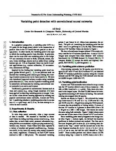
Fig. 2. Defective samples from public DAGM data set. Defect positions are marked by red circles.

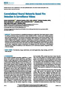
Fig. 1. Triplet network: Images a, b, and c fed into the same network. Samples a and b belong to the same class, sample c belongs to a different class. After computing the features for each input, distance d1 between the same-class samples and distance d2 between samples a and c are computed. Both distances are then concatenated to form a vector. This vector is then subjected to the softmax function restricting output values to lie between zero and one.

Subsequently the results for d1 and d2 are concatenated and normalized so that their sum is equal to one (i.e. the softmax function), yielding the output vector

𝑝 = 𝑠𝑜𝑓𝑡𝑚𝑎𝑥 𝑑1 , 𝑑2 The network is then trained with the target vector [0,1] for each triplet of (a,b,c). The triplet network setup is illustrated in figure 1. 2.2. Defect Detection Pipeline We first train a CNN to learn similarities between patches of 32×32 pixels. For defect detection we then create a prototype by extracting the features for a large amount of nondefective data and calculating the mean feature values. For each new measurement we then calculate the distance between the prototype and the measurement features. All networks are built fully convolutional. This way they can also process larger resolution input, extracting features for each 32×32 neighborhood.

The second data we refer to as the public DAGM data set. It was published by the German Association for Pattern Recognition (DAGM) in the context of a competition on surface defect detection from weakly labeled data [19]. The data set consists of 6 texture classes with 1000 non-defective and 150 defective samples. For training we use 500 of the non-defective samples from each class. The third data set is the CIFAR100 data set [20] which contains 60000 color images of 32×32 resolution. There are 100 different classes with 600 samples each. For this work we transformed the images to grayscale. This data set was included to test the hypothesis that learning the more complex similarities between objects also leads to better features for texture anomaly detection. 2.4. Evaluation data For evaluation we use two data sets: The first data set consists of the defective samples from the public DAGM data set, as well as the 500 non-defective samples from each class that were not used for training. In order to evaluate performance on novel defect classes we used the second part of the DAGM data set that was used for the final competition. We will refer to it as the competition DAGM data set. It consists of 4 additional texture classes with 2000 nondefective and 300 defective samples each. Samples are shown in figure 2. 2.5. Data Preprocessing For network training, all images are resized to 512x512 pixel resolution and then scaled to values from -1 to 1.

2.3. Training data For training the networks we use combinations of three different data sets. The Kylberg Texture Dataset v1.0 [18] contains 28 texture classes, each consisting of 160 grayscale images at 576×576 pixels resolution.

Fig. 2. Defective samples from competition DAGM data set. Defect positions are marked by red circles.


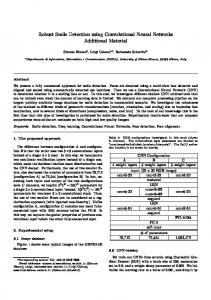
Fig. 3. Left to right: Input texture and corresponding patches of 32×32 pixels for decreasing input sizes.

From the resulting images, patches of 32x32 pixels were sampled at random positions. The patch size was chosen based on previous work showing that this is sufficient for defect classification in the DAGM data set [10]. As some surface classes exhibit a global pattern we sampled the same-class images at the same positions as the input image, ensuring that patches are compared at the same position. 2.6. Data Augmentation We employed two types of data augmentation to artificially increase the amount of texture data. The first type of data augmentation uses the fact that textural regularities are expressed on different spatial scales, i.e. some patterns are easily recognizable when looking at patches of 32×32 pixels while others can only be identified when looking at larger image areas (see figure 3). To incorporate this variety into the training data, while keeping the patch size fixed at 32×32, we randomly resized the input images to either 512×512, 256×256, 128×128 or 64×64 pixels. For the second type of data augmentation we artificially corrupted same-class samples with patches of Gaussian noise and labelled the results as out-of-class samples. This is inspired by the random erasing data augmentation approach [21], but with the opposite aim, i.e. instead of decreasing sensibility to local deviations our aim is to increase sensibility to local deviations. Data augmentation was only applied to texture images, i.e. the CIFAR-100 data set was not subjected to data augmentation. 2.7. Network parameters In this work we use a simple architecture based on the idea of deep residual learning [5]. The rationale behind this idea is that instead of learning a set of new representations at each layer, a residual with respect to the input layer is learned. Architectures like this idea have shown to be easier to optimize even with deeper networks [5]. The basic component are residual blocks. Table 1 shows the setup and parameters of the residual block used in this work.

Input resolution (H: height, W: width)

inp

-

-

-

H×W×h

-

Conv2D

L1

5×5

elu

inp

H×W×h

H-4×H-4×h

Conv2D

L2

1×1

linear

L1

H-4×H-4×h

H-4×H-4×h

Cropping2D

L3

-

-

inp

H×W×h

H-4×H-4×h

Addition

L4

-

-

L2,L3

H-4×H-4×h

H-4×H-4×h

Input(s)

Output resolution

name

input

Activation

Layer type

Window size

Table 1. Residual block setup and parameters

Each residual block consists of one convolutional layer with a non-linear activation function followed by a convolutional layer with linear activation function, a cropping function and an addition operation. The first convolutional layer thereby learns a set of 5×5 filters. Due to border effects the outputs spatial resolution is reduced by two at each border (up/down,left/right). The purpose of the second convolutional layer is to allow the learned residual to cover positive and negative values equally, which is why its filter size is set to 1×1 and the activation function is linear. The purpose of the cropping function is to adjust the spatial scale of the input so that the learned residual can be added. The final network uses one initial convolutional layer with filter size of 7×7, followed by a max-pooling operation with window size of 2×2 and strides of 2×2. The max-pooling thereby samples the input down by a factor of 0.5. The result is processed by three residual blocks, followed by a convolutional layer with filter size of 1×1. All but the first and the last layer have filter sizes of 5×5. The last layers purpose is to allow the final representation to cover both positive and negative values equally, which is why its filter size is 1×1 and the activation function is linear. All other layers use the exponential linear unit (elu) as activation function [22]. The elu activation function was picked to avoid the use of batch normalization [23], as this has caused problems in our initial attempts. All layers used the same amount of units h with either h=16 or h=32. All networks were implemented to be fully convolutional so that they can easily be used to process larger resolution input. Due to the max-pooling operation and border effects in convolutional layers input images of 512×512 pixels are thereby transformed into feature tensors with dimensions 241×241×h. Table 2 summarizes the setup of the networks used in this work. Table 2. Network parameters. Layer type

Window size

Activation function

Input resolution

Output resolution

Conv2D

7×7

elu

32×32×1

26×26×h

Max-pooling2D ResBlock

2×2

-

26×26×h

13×13×h

5×5

elu

13×13×h

9×9×h

ResBlock

5×5

elu

9×9×h

5×5×h

ResBlock

5×5

elu

5×5×h

1×1×h

Conv2D

1×1

linear

1×1×h

1×1×h


2.8. Optimization/Training Hoffer et al. [11] found that minimizing mean squared error (mse) yielded better results than minimizing categorical cross entropy. Here we use mean absolute error (mae) because assuming that the network starts with random guesses the error will be ≤ 1 for the largest portion of training. The mae should therefore allow for faster convergence. We used the Adam optimizer [24] with learning rate fixed at 0.0001 and a batch size of 256 samples. The networks were trained for 6×15 epochs: A different set of triplets was sampled after fifteen epochs of training and this process was repeated six times. All networks are implemented using the keras library [25] for Python and tensorflow [26]. 2.9. Evaluation

3. Results Figure 4 shows defect detection examples for all ten classes. Table 3 shows the area under the curve (auc) scores for all classes and experiments. It can be seen that performance varies a lot depending on the surface type. While the best results for classes one, three, five and six reach performances that are useful for an industrial application, the method fails to discriminate defective and non-defective areas for classes two and four. It can further be seen that the training data has considerable effect on the defect detection performance. Adding samples from CIFAR-100 to the training data improves overall performance, especially for the novel surface classes from the competition DAGM data set.

Fig. 4. Defect detection examples. Upper row: Classes 1-5 with input sample in gray on top and heatmap of Euclidean distance from prototype at the bottom (blue for low values and red for high values). Lower row: Classes 610 with input sample in on top and heatmap of Euclidean distance from prototype at the bottom. Table 3. Results: median ± standard deviation of area under curve (auc) for three experiments auc score: median ± standard deviation

Known surface

Class

novel surface

We train three different networks for each set of parameters, i.e. number of units h=16/32 as well as with/without samples from the CIFAR data set in the training data. For evaluating defect detection performance, we use both the public and the competition DAGM data sets. Prototypes are created by feeding 500 non-defective samples for each class into the network and taking the mean over the resulting features. For each of the remaining defective and non-defective samples we then calculate the Euclidean distance from the prototype, yielding a distance matrix of dimensions 241×241. To assess how well nondefective and defective samples are discriminated we compute the maximum value for each distance matrix and calculate the amount of true positives and false positives for varying thresholds. True positives thereby denote defective samples correctly classified as defective and false positives denote non-defective samples wrongly classified as defective. The results are expressed as receiver-operating characteristic (ROC) curves. To assess the performance of each network in a single number we calculate the area under the ROC curve (auc). As summary statistics over the three networks trained for each set of parameters we used median and standard deviation.

h = 16

h = 16, +cifar

h = 32

h = 32, +cifar

1

0.99±0.01

0.98±0.01

0.99±0.03

0.93±0.03

2

0.48±0.02

0.47±0.02

0.47±0.0

0.45±0.01

3

0.72±0.04

1.0±0.003

0.84±0.03

1.0±0.003

4

0.66±0.07

0.49±0.02

0.56±0.02

0.51±0.08

5

1.0±0.002

1.0±0.0

1.0±0.0

1.0±0.0

6

0.97±0.02

0.98±0.02

0.98±0.0

1.0±0.03

7

0.76±0.09

0.95±0.14

0.79±0.08

0.61±0.16

8

0.93±0.03

1.0±0.0

0.99±0.03

1.0±0.0

9

0.51±0.03

0.98±0.03

0.61±0.12

0.86±0.07

10

0.56±0.01

0.57±0.03

0.54±0.02

0.63±0.09

0.76

0.83

0.78

0.81

mean

Regarding network parameters we find no clear difference between using 16 or 32 units, i.e. setting h=16 or h=32. Generally, the method translates well to novel inputs as it is able to achieve very good discrimination for classes eight and nine and good discriminative power for class seven. 4. Discussion Here we show for the first time how deep metric learning can be used for surface anomaly detection. The results are promising but also leave room for further improvement. We found that adding data from the CIFAR100 data set allows for learning more powerful features. Similar findings have been reported before, where models trained on more complex object classification tasks outperformed models trained only with textures [27]. A possible direction for future work is hence to test whether a network trained on both object and


texture images actually outperforms a network trained only on object images. One remaining problem is, that while reaching perfect discrimination for some classes, the method completely fails for other classes. While we did not find a difference in performance depending on the amount of units h in each layer and hence the dimensionality of the representation learned by the network, it is known that the Euclidean distance is not necessarily a good choice when dealing with highdimensional data [28]. Further investigation into the use of alternative distance measures, like e.g. Manhattan distance, could hence have a positive impact on the results. Other potential remedies are the use of larger image patches, increasing the amount and complexity of the training data and further investigations into alternative CNN architectures and hyperparameters. Acknowledgements The authors gratefully acknowledge the financial support by Deutsche Forschungsgemeinschaft (DFG, German Research Foundation) for subproject B5 "safe processes" within the SFB 747 (Collaborative Research Center) "Micro Cold Forming - Processes, Characterization, Optimization".

References [1] Flosky H, Vollertsen F. Wear behaviour in a combined micro blanking and deep drawing process. CIRPAnnals-Manufacturing Technology 2014; 63.1: 281-284. [2] Xie X. A review of recent advances in surface defect detection using texture analysis techniques. ELCVIA Electronic Letters on Computer Vision and Image Analysis 2008; 7.3: 1-22. [3] Neogi N, Mohanta DK, Dutta PK. Review of vision-based steel surface inspection systems. EURASIP Journal on Image and Video Processing, 2014; 1:50-69. [4] Krizhevsky A, Sutskever I, Hinton GE. Imagenet classification with deep convolutional neural networks. Advances in neural information processing systems 2012; 1097-1105. [5] He K, Zhang X, Ren S, Sun J. Deep residual learning for image recognition. Proceedings of the IEEE conference on computer vision and pattern recognition 2016; 770-778. [6] Long J, Shelhamer E, Darrell T. Fully convolutional networks for semantic segmentation. Proceedings of the IEEE conference on computer vision and pattern recognition 2015; 3431-3440. [7] Ren S, He K, Girshick R, Sun J. Faster r-cnn: Towards real-time object detection with region proposal networks. IEEE Transactions on Pattern Analysis & Machine Intelligence 2017; 6: 1137-1149. [8] Masci J, Meier U, Ciresan D, Schmidhuber J, Fricout G. Steel defect classification with max-pooling convolutional neural networks.

International Joint Conference on Neural Networks Neural Networks (IJCNN) 2012; 1-6. [9] Soukup D, Huber-Mörk R. Convolutional neural networks for steel surface defect detection from photometric stereo images. International Symposium on Visual Computing 2014;668-677. [10] Weimer D, Scholz-Reiter B, Shpitalni M. Design of deep convolutional neural network architectures for automated feature extraction in industrial inspection. CIRP Annals 2016; 65.1:417-420. [11] Hoffer E, Ailon N. Deep metric learning using triplet network. International Workshop on Similarity-Based Pattern Recognition 2015; 84-92. [12] Schroff F, Kalenichenko D, Philbin J. Facenet: A unified embedding for face recognition and clustering. Proceedings of the IEEE conference on computer vision and pattern recognition 2015; 815-823. [13] Pimentel MA, Clifton DA, Clifton L, Tarassenko L. A review of novelty detection. Signal Processing 2014; 99:215-249. [14] Natarajan V, Hung TY, Vaikundam S, Chia LT. Convolutional networks for voting-based anomaly classification in metal surface inspection. IEEE International Conference on Industrial Technology (ICIT) 2017;986-991. [15] Napoletano P, Piccoli F, Schettini R. Anomaly Detection in Nanofibrous Materials by CNN-Based Self-Similarity. Sensors 2018; 18.1:209. [16] Song HO, Xiang Y, Jegelka S, Savarese S. Deep metric learning via lifted structured feature embedding. IEEE Conference on Computer Vision and Pattern Recognition (CVPR) 2016; 4004-4012 [17] Hermans A, Beyer L, Leibe B. In defense of the triplet loss for person re-identification. arXiv preprint 2017; arXiv:1703.07737. [18] Kylberg G. The Kylberg Texture Dataset v. 1.0, Centre for Image Analysis, Swedish University of Agricultural Sciences and Uppsala University, External report (Blue series) No. 35. Available online at: http://www.cb.uu.se/~gustaf/texture/ [19] Weakly Supervised Learning for Industrial Optical Inspection. 29th Annual Symposium of the German Association for Pattern Recognition. https://resources.mpi-inf.mpg.de/conference/dagm/2007/prizes.html [20] Krizhevsky A, Hinton G. Learning multiple layers of features from tiny images. Technical report, University of Toronto 2009; 1.4:7-67 [21] Zhong Z, Zheng L, Kang G, Li S, Yang Y. Random Erasing Data Augmentation. arXiv preprint 2017; arXiv:1708.04896. [22] Clevert DA, Unterthiner T, Hochreiter S. Fast and accurate deep network learning by exponential linear units (elus). arXiv preprint 2015; arXiv:1511.07289. [23] Ioffe S, Szegedy C. Batch normalization: Accelerating deep network training by reducing internal covariate shift. arXiv preprint 2015; arXiv:1502.03167. [24] Kingma DP, Ba J. Adam: A method for stochastic optimization. arXiv preprint 2014; arXiv:1412.6980. [25] Chollet, F. Keras. Github (https://github.com/fchollet/keras) 2015 [26] Abadi M, Barham P, Chen J, Chen Z, Davis A, Dean J, Kudlur, M. TensorFlow: A System for Large-Scale Machine Learning. OSDI 2016; 16: 265-283. [27] Cusano C. Napoletano P, Schettini R. Combining multiple features for color texture classification. J. Electron. Imaging 2016; 25.6:061410. [28] Aggarwal CC, Hinneburg A, Keim DA. On the surprising behavior of distance metrics in high dimensional space. International conference on database theory 2001; 420-434.