3198
IEEE TRANSACTIONS ON MAGNETICS, VOL. 37, NO. 5, SEPTEMBER 2001
Application of a Meshless Method in Electromagnetics S. L. Ho, S. Yang, J. M. Machado, and H. C. Wong
Abstract—An improved meshless method is presented with an emphasis on the detailed description of this new computational technique and its numerical implementations by investigating the usefulness of a commonly neglected parameter in this paper. Two approaches to enforce essential boundary conditions are also thoroughly investigated. Numerical tests on a mathematical function is carried out as a means of validating the proposed method. It will be seen that the proposed method is more robust than the conventional ones. Applications in solving electromagnetic problems are also presented. Index Terms—Lagrange multiplier method, least squares method, meshless method, moving-least square approximants.
I. INTRODUCTION
M
ESHLESS methods, originated about twenty years ago, are now proven as a robust technique to study field problems in which large geometrical deformations are to be modeled [1]–[3], since such methods avoid the onerous mesh generation and adaptive updating, thereby resulting in continuous differentiable approximations that are smooth functions and require no post-processing. In simulation studies in electrical engineering, it is common to have geometrical deformations for optimization and nondestructive evaluation problems, and many researchers have found the meshless method very promising for the study of electromagnetics [4]–[6]. This paper describes in details the discretization procedures and the associated discrete formulations of a meshless method based on the Moving Least Square (MLS) approximant that are required when using meshless methods to study electromagnetic problems. The special techniques for enforcing essential boundary conditions and for approximating the discontinuous derivatives on the interface of different materials are also investigated. A factor which contributes a significant difference which is omitted by most related meshless methods is also pointed out. To validate the new formulation, a set of thorough numerical results are presented and compared with those obtained from a mathematical function. Some numerical experiences and suggestions are also highlighted for facilitating the
application of this new computational technique in electrical engineering. II. MESHLESS METHOD USING MLS Although the theoretical contents of meshless methods have been fully demonstrated by many researchers in related fields [1]–[3], it is felt that there is still a need to give a detailed description of the method to improve understanding of this new computational technique by fellow researchers. A. Governing Equation and Weak Form Functional For illustrative purposes, one considers two dimensional magneto/electrostatic problems which are governed by the equation of equilibrium (1) The essential and natural boundary conditions are, respectively, (2) (3) , is the boundaries of . where The weak form functional corresponding to the above boundary value problem is
(4) Owing to the non-Kronecker delta function property of the shape functions of meshless methods, an additional term representing contributions of normal derivatives of the solution variable on essential boundaries that corresponds to that for the finite element method, is introduced in the formulations of (4). It should be pointed out that this term is commonly neglected by most fellow researchers in their related works. B. Moving Least Square Approximations
Manuscript received June 6, 2000. S.L. Ho is with the EE Department, the Hong Kong Polytechnic University, Hong Kong (e-mail:
[email protected]). S. Yang was with the EE Department, Zhejiang University, and is now with the EE Department, the Hong Kong Polytechnic University, Hong Kong (e-mail:
[email protected]). J. M. Machado is with Universidade Estadual Paulista, S.J.do Rio Preto, Brazil (e-mail:
[email protected]). H. C. Wong is with the Industrial Center, the Hong Kong Polytechnic University, Hong Kong (e-mail:
[email protected]). Publisher Item Identifier S 0018-9464(01)07963-8.
In the proposed method, the trial and test functions for the variational principle are constructed by using moving least square approximations entirely in terms of a set of nodes, i.e., (5) will vary with where the unknown parameters is the basis of a complete polynomial of order .
0018–9464/01$10.00 © 2001 IEEE
Authorized licensed use limited to: Hong Kong Polytechnic University. Downloaded on March 14, 2009 at 10:51 from IEEE Xplore. Restrictions apply.
and
HO et al.: APPLICATION OF A MESHLESS METHOD IN ELECTROMAGNETICS
For two dimensional problems, , and a linear is used in this paper. basis , the difference To determine the unknown parameters between the local approximation given by (5) and the nodal panorm as given by (6), rameters , i.e., the weighted, discrete is minimized. Moreover,
(6) is a compactly supported weighting where and is the number of nodes in function with center at node the neighborhood of for which the weighting function [3], [4]. The weighting functions used in this paper are the tensor products of one dimensional ones. Minimization of (6) with releads to the following linear equation set spect to (7) , , For the special case where a linear basis is used, become, respectively,
where,
3199
different material interfaces, the approximation of (10) then becomes (12) where is the jump function which will generate the discontinuous normal derivatives, is the distance to the closest point on the interface line segment of discontinuity, and is positive on one side and negative on the other side of the interface line section. The spline jump function is used in this paper to generate the discontinuous normal derivatives, and the details about this jump function and its numerical implementation are given in [7]. In order to simplify the development of the discrete equation set in what follows, one will use the form of (10) to approximate the solution variable. However one must also note that includes both the shape function and the jump shape function . D. Discrete Equations
. and
(8)
(9) from (7) and then substituting it to (5), then the Solving moving least square approximant is given by (10) is defined as the shape function of the MLS apwhere proximants, and is determined by using
As in the general case of meshless methods, the application of essential boundary conditions is very complicated and difficult since the shape functions do not satisfy the Kronecker delta criterion. Two different approaches, i.e., the collocation and Lagrange multiplier methods, are investigated in this paper. Numerical experiences show however that the collocation method could not be used simply in the meshless methods. Instead, an improved form of it, the least squares approach, is proposed in this paper because of its simplicity when it comes to numerical implementation. The difference in the approaches to impose essential boundary conditions will result in some small differences in discrete equations. 1) Discrete Equations Using Lagrange Multiplier Method to Enforce Essential Boundary Conditions: In this case, the Lagrange Multiplier Method is used to enforce the essential boundary conditions. The modified functional of (4) needed to be minimized then becomes [8] (13)
(11)
where
is the Lagrange Multiplier and can be expressed as (14)
C. Interface Condition Approximation Although the continuous approximation of the (partial) derivatives of the solution variable is considered as having the promising characteristics of meshless methods, it also has a drawback in engineering problems where the solution variable do have discontinuities of (partial) derivatives at, for example, the interface of different materials, since the continuous differentiable approximations will lead to the solution variable exhibiting the well known Gibb’s phenomenon in the interfaces. Here the jump function approach is used [7]. The basic idea of this approach is that some special shape functions are introduced in the interfaces of different materials so as to generate the required discontinuous normal derivatives. For line segments of example, considering a problem with
is a Lagrange interpolant and is the arc length where along the boundary. From the necessary condition for (13) to reach its minimum, one obtains
Authorized licensed use limited to: Hong Kong Polytechnic University. Downloaded on March 14, 2009 at 10:51 from IEEE Xplore. Restrictions apply.
(15) (16)
3200
IEEE TRANSACTIONS ON MAGNETICS, VOL. 37, NO. 5, SEPTEMBER 2001
Substituting (10) and (14) into (15) and (16), letting , , and then integrating, one obtains (17) where (18) (19) (20) (21) where
Fig. 1. Comparison between analytical and numerical solutions for the mathematical function using Largrange multiplier method to impose essential boundary conditions with and without considering the contributions of nonzero normal derivatives of the solution variable on essential boundaries.
(22) must be Just as mentioned previously, an additional term introduced to the right hand side of the discrete equations when one considers the contributions of the nonzero normal derivatives of the solution variable on the essential boundaries. Unfortunately, this term is commonly ignored in most of the related works [1]–[3]. 2) Discrete Equation Using Least Squares Method to Impose Essential Boundary Conditions: The collocation method cannot be used easily to enforce essential boundary conditions in meshless methods. Thus an improved form of it, the least squares approach, is used as an alternative to incorporate essential boundary conditions. The minimization of (4) results in the following discrete equations (23) where and are, respectively, defined in (18) and (20). For the approximants (10) to satisfy the essential boundary condition (2), the following discrete equations are used: (24) is the total node number on the boundary , and where is the coordinates of the corresponding th node. Due to the fact that the number of the total equations of (23) and (24) is greater than the freedom of coefficients , the solution of is obtained by minimizing the following residual with respect to .
Fig. 2. Comparison between analytical and numerical solutions for the mathematical function using the collocation method to enforce essential boundary conditions with and without considering the contributions of nonzero normal derivatives of the solution variable on essential boundaries.
III. NUMERICAL EXAMPLES A. Numerical Validation In order to validate the proposed method, a one dimensional mathematical function with analytical solutions is solved [3]. The problem is to find the solution of (26) and
(27)
. The exact solution of (26) and (27) is , the following It is obvious that at the essential boundary nonzero normal derivative of the solution variable exists, (28)
(25)
This problem is solved by using the proposed method under four different cases, namely, cases where Lagrange multiplier method is used to enforce essential boundary conditions with and without considering the contributions of (28), and cases in which the least squares method is used to impose the essential boundary conditions with and without considering
Authorized licensed use limited to: Hong Kong Polytechnic University. Downloaded on March 14, 2009 at 10:51 from IEEE Xplore. Restrictions apply.
HO et al.: APPLICATION OF A MESHLESS METHOD IN ELECTROMAGNETICS
Fig. 3. A parallel plate capacitor.
Fig. 4.
3201
Fig. 6. Comparison of computed and exact solutions for the parallel plate capacitor.
An infinite square ground metal slot. Fig. 7.
The computed equipotential contours of the ground metal slot.
TABLE I PERFORMANCE COMPARISON OF THE MESHLESS AND FINITE ELEMENT METHODS FOR THE 2-D PROBLEM RUNNING IN A 600 MHZ MACHINE (a)
(b)
Fig. 5. Nodal arrangement and background integration cell for the 2-D problem: (a) nodal arrangement; (b) integration cell.
the contribution of (28). In the numerical computations, 11 equi-distance nodes are used, and the weighting function used is a cubic spline one [3]. The comparisons of numerical results with the exact ones for different cases are given in Figs. 1 and 2. From these results one can see that: (1) as revealed by Fig. 2, by considering contributions of the nonzero normal derivative , the of the solution variable on the essential boundary proposed method based on the least squares method to enforce the essential boundary conditions gives “almost exactly” numerical results for both the solution variable and its derivative, although only 11 equi-distance nodes are used. When excluding this contribution, other things being equal, the method will lead to fictitious numerical results; (2) as demonstrated in Fig. 1, the computed results of the proposed method based on Lagrange multiplier method to impose essential boundary conditions under two different cases, i.e., whether the contribution of
the nonzero normal derivative of the solution variable on the essential boundary is considered or not, are almost the same and show good agreement with the exact solutions. However, the computed Lagrange multipliers in the two different cases and . are, respectively, B. Application The proposed method is used to study both 1-D and 2-D field problems, i.e., to determine the fields of a parallel plate capacitor with a uniform permittivity between the plates (Fig. 3), and to determine the fields of an infinite square grounding metal slot (Fig. 4). In the numerical implementation, the cubic spline function is also used as the weight function, 11 equi-distance nodes are used for the 1-D problem, and the nodal arrangement and the background integration cells for the 2-D problem are shown in Fig. 5. The comparison between the analytical and the computed solutions for the 1-D problem is given in Fig. 6, and the equipotential contours obtained by using the proposed method for the 2-D problems is shown in Fig. 7. The performance comparisons between the finite element and the proposed methods for the 2-D problem is given in Table I. From these results it can be seen that (1) the computed results of the 1-D problem agree well with the analytical solutions, and (2) the proposed method is competitive to finite element methods although the CPU time used by the proposed method is much longer compared with that
Authorized licensed use limited to: Hong Kong Polytechnic University. Downloaded on March 14, 2009 at 10:51 from IEEE Xplore. Restrictions apply.
3202
IEEE TRANSACTIONS ON MAGNETICS, VOL. 37, NO. 5, SEPTEMBER 2001
of the finite element method considering the fact that the numerical solver of MATLAB for the large sparse equation set used in the proposed meshless method is not as efficient as that, i.e., ICCG, used for the finite element method.
Multiplier Method and those combinations of the finite element and the meshless methods that are not so sensitive to these contributions. REFERENCES
IV. CONCLUSION A detailed description of a meshless method and its numerical implementation is presented. A significant difference between the finite element and meshless methods lies in a parameter which is commonly neglected in most related works. An improved formulation is thus derived. The presented numerical results show that: (1) the contributions of nonzero normal derivatives of the solution variable on the essential boundaries, as a general rule, must be included in the discrete equation set of meshless methods; (2) the improved formulation with the aforementioned contributions presented in this paper is more robust than the traditional ones; (3) one must keep in mind that the normal derivatives of the solution variable on essential boundaries are also important when one applies the meshless methods. Alternatively, it is suggested that one should select formulations such as those based on the Lagrange
[1] T. Belytschko, Y. Krongauz, D. Organ, M. Fleming, and P. Krysl, “Meshless method: an overview and recent development,” Comput. Methods Appl. Mech. Engrg., vol. 139, pp. 3–47, 1996. [2] T. Belytschko, Y. Y. Lu, and L. Gu, “Element-free Galerkin methods,” Int. J. Numer. Engrg, vol. 37, pp. 229–256, 1994. [3] J. Dolbow and T. Belytschko, “An introduction to programming the meshless element free Galerkin method,” Archives of Computational Methods in Engineering, vol. 5, no. 3, pp. 207–241, 1998. [4] V. Cingoski, N. Miyamoto, and H. Yamashita, “Element-free Galerkin method for electromagnetic field computations,” IEEE Trans. Magn., vol. 34, no. 5, pp. 3236–3239, 1998. [5] S. A. Viana and R. C. Mesquita, “Moving least square reproducing Kernel method for electromagnetic field computation,” IEEE Trans. Magn., vol. 35, no. 3, pp. 1372–1375, 1999. [6] C. Herault and Y. Marechal, “Boundary and interface conditions in meshless methods,” IEEE Trans. Magn., vol. 35, no. 3, pp. 1450–1453, 1999. [7] Y. Krong and T. Belytschko, “EFG approximation with discontinuous derivatives,” Int. J. Numer. Engrg., vol. 41, pp. 1215–1233, 1998. [8] J. N. Reddy, An Introduction to Finite Element Method: McGraw-Hill, Inc., 1993.
Authorized licensed use limited to: Hong Kong Polytechnic University. Downloaded on March 14, 2009 at 10:51 from IEEE Xplore. Restrictions apply.