1078
JOURNAL OF APPLIED METEOROLOGY
VOLUME 44
Application of a Multigrid Method to a Mass-Consistent Diagnostic Wind Model YANSEN WANG, CHATT WILLIAMSON, DENNIS GARVEY, SAM CHANG,
AND
JAMES COGAN
U.S. Army Research Laboratory, Adelphi, Maryland (Manuscript received 27 April 2004, in final form 1 February 2005) ABSTRACT A multigrid numerical method has been applied to a three-dimensional, high-resolution diagnostic model for flow over complex terrain using a mass-consistent approach. The theoretical background for the model is based on a variational analysis using mass conservation as a constraint. The model was designed for diagnostic wind simulation at the microscale in complex terrain and in urban areas. The numerical implementation takes advantage of a multigrid method that greatly improves the computation speed. Three preliminary test cases for the model’s numerical efficiency and its accuracy are given. The model results are compared with an analytical solution for flow over a hemisphere. Flow over a bell-shaped hill is computed to demonstrate that the numerical method is applicable in the case of parameterized lee vortices. A simulation of the mean wind field in an urban domain has also been carried out and compared with observational data. The comparison indicated that the multigrid method takes only 3%–5% of the time that is required by the traditional Gauss–Seidel method.
1. Introduction Numerical modeling of transport and diffusion or analysis of atmospheric effects on the performance of sensors requires wind data with high spatial (10–100 m) and temporal (2–5 min) resolution in a reasonably large (10 km ⫻ 10 km) domain. While increasing the resolution, or nesting a large-eddy simulation model within a mesoscale weather model (which can provide mean values and associated turbulence statistics), is a potential solution for the requirement, it remains impractical for real-time applications in a domain with a large number of grid points in the foreseeable future because of the limitations of computational power. For applications requiring rapid but reasonably accurate results, a welldesigned diagnostic model, exercised at specific times over limited domains, may provide a solution. One particular type of diagnostic model, which satisfies the mass-consistent constraint, is explored in this study. The theoretical basis for this type of model was developed by Sasaki (1958, 1970), using variational analysis. There have been many developments and applications of this type of model during the last several
Corresponding author address: Dr. Y. Wang, U.S. Army Research Laboratory, ATTN: AMSRD-ARL-CI-EB, 2800 Powder Mill Road, Adelphi, MD 20783. E-mail:
[email protected]
JAM2262
decades. Sherman (1978) and Dickerson (1978) applied mass conservation to an analysis of atmospheric flows over complex terrain. Their model used a local Cartesian coordinate system, and the earth’s surface was approximated with a constant step in the vertical direction. The partition of flow into vertical and horizontal directions used a simple empirical coefficient. Another development of such a model by Davis et al. (1984) and Ross et al. (1988) employed a terrain-following sigma-z coordinate system. Connell (1988) has done extensive tests on Ross’s model using observational data. These authors attempted to formulate the flow partition coefficient in terms of the Froude number. Kitada et al. (1986) adopted a similar coordinate system in their model. The model was applied to the wind circulation in a land–sea breeze simulation. Moussiopoulos and Flassak (1986) presented a faster numerical algorithm in a vector computer to compute the wind field. Venkatesan et al. (1997) have incorporated an objective analysis technique into a mass-consistent model, and the results showed improvement in modeling flow past a hill. In many turbulent transport and diffusion models, a mass-consistent model has been applied to physically interpolate the wind field in high-resolution computational grids using limited observation profiles or mesoscale model simulation results. Ratto (1996) has provided a recent literature review on mass-consistent models over complex terrain. He points out that a mass-
JULY 2005
1079
WANG ET AL.
consistent model provides similar performances when compared with a full dynamical simulation model in some applications. The earlier models typically cover 100 km ⫻ 100 km domains at horizontal resolutions of 2–4 km. A partition of flow in the horizontal and vertical directions is needed to account for the weaker vertical wind component in a coarse resolution. Massconsistent models have also been applied in many objective analysis techniques to correct for the excessive divergence in initial wind fields for meso- or large-scale numerical weather prediction models (Liu and Goodin 1976; Brocchini et al. 1995). Recently, mass-consistent diagnostic models have been applied to simulate the wind field in urban environments, and wakes and vortices near buildings have been parameterized (Röckle 1990; Kastner-Klein et al. 2001; Pardyjak and Brown 2002; Brown 2004). The mathematical formulation in the mass-consistent model is a Poisson equation for the Lagrange multiplier as described below. All models reviewed above employ the traditional Gauss–Seidel (GS) iteration method. The convergence of the method is too slow for realtime simulations when a domain has a large number of grid points. In recent years, the multigrid method has been used widely in solving the Poisson equation. There are several other popular iterative methods to solve the linear systems, such as the strongly implicit (SIP) method, the alternating direction implicit (ADI) method, and the conjugate gradient (CG) method. The multigrid method has been applied in the GS and SIP methods to accelerate the speed of convergence and to condition the matrix in the CG method. The efficiency of the multigrid method is reviewed in Wesseling (1992). The origin of the multigrid method is found in Fedorenko (1961), and later in Bakhvalov (1966) and Brandt (1977). A fairly complete reference to the multigrid work can be found in Wesseling (1992) and Briggs et al. (2000). In the last two decades, the application of this method has mushroomed in computational fluid dynamics and has proven to be one of the fastest methods to solve elliptic-type equations. The objective in this paper is to describe a robust, high-resolution three-dimensional mass-consistent diagnostic wind model, named the three-dimensional wind field (3DWF) model, which has been developed at the U.S. Army Research Laboratory. The focus of this paper is to apply a multigrid method to speed up the numerical solution of the model so that the model can be run in real-time simulations on a personal computer (PC) platform. A very brief description of the model framework and a detailed numerical implementation of the multigrid method in the model is discussed in section 2; an idealized test with an analytical solution, an
application of the method in a real world simulation in complex terrain with parameterization of lee vortices, and a test with an urban wind observation are presented in section 3.
2. Numerical implementation of the model a. A brief description of the model The mass-consistent model is based on the principle of mass conservation in which divergence is eliminated in a flow field. Given a limited number of observations or a coarsely modeled wind field over complex terrain, the wind field is physically interpolated in such a way that mass conservation is satisfied. Mathematically, the problem is to minimize the functional (Sasaki 1958, 1970; Sherman 1978)
冕冋 冉
E共u, , w, 兲 ⫽
21共u ⫺ u0兲2 ⫹ 21共 ⫺ 0兲2 ⫹ 22共w ⫺ w0兲2
V
⫹
⭸u ⭸ ⭸w ⫹ ⫹ ⭸x ⭸y ⭸z
冊册
共1兲
dx dy dz,
where x, y are the horizontal coordinates; z is the vertical coordinate; u0, 0, and w0 are the initial observed velocity components; u, , and w are the corrected velocity components; is the Lagrange multiplier; and 1 and 2 are Gauss precision moduli, which are the wind vector–partitioning factors in the horizontal and vertical directions. The integral domain of the model is V. The corresponding Euler–Lagrange equations can be derived (Sherman 1978). The resulting equation for is a Poisson equation: ⭸2 ⭸x
2
⫹
⭸2 ⭸y
2
⫹ ␣2
⭸2 ⭸z
2
⫽ ⫺2
冉
冊
⭸u0 ⭸0 ⭸w0 ⫹ ⫹ . ⭸x ⭸y ⭸z
共2兲
The value in Eq. (2) can be solved numerically by setting the boundary conditions on all facets of the computation domain. The u, , w wind components then can be computed from the Euler–Lagrange equations using the value solved from Eq. (2). The iterative convergence will be the high-resolution diagnostic solution for u, , and w for given boundary and coarse initial conditions (observations). At the lateral and top boundaries, is set equal to zero to allow “flow through” in the flow adjustment. At the bottom of the domain “no–flow through” conditions can be satisfied by having the normal derivative vanish, that is, /n ⫽ 0, where n is the normal to an impermeable surface. A detailed description on the mass-consistent wind model is referred to in Sherman (1978) and other literatures reviewed in the introduction section. The deficiency of a mass-consistent model is that it is unable to simulate the vortices or wakes in the lee of
1080
JOURNAL OF APPLIED METEOROLOGY
steep topography because the momentum conservation is not included. However, features of this kind can be parameterized or inserted in the initial field according to observational studies (Hunt and Snyder 1980; Snyder et al. 1985; Connell 1988; Brown et al. 2000; KastnerKlein et al. 2001). The effect of vegetation canopies (Cionco 1965) will also be parameterized in further development of the model.
b. Numerical method using multigrid method Equation (2) is discretized using a standard sevenpoint method with second-order accuracy in all three spatial directions,
i⫹1,j,k ⫺ 2i,j,k ⫹ i⫺1,j,k 共⌬x兲
2
⫹ ␣2
⫹
i,j⫹1,k ⫺ 2i,j,k ⫹ i,j⫺1,k
i,j,k⫹1 ⫺ 2i,j,k ⫹ i,j,k⫺1 共⌬z兲2
共⌬y兲2
⫽ ⫺2f0,
共3兲
where f0 is the divergence of the wind field in the previous iteration (or the initial divergence in the case of the first iteration). The divergence term can be discretized using a central difference scheme. The flowthrough boundary conditions are set by letting ⫽ 0, the no-flow-through boundary conditions at the terrain surface or the building walls are applied by setting the normal derivative at the point to zero using a threepoint difference with second-order accuracy. The adjusted wind field is then computed from the following equation (Sherman 1978): 1 0 0 0 ⫹ 2ui,j,k ⫹ ui⫺1,j,k ui,j,k ⫽ 共ui⫹1,j,k 兲 4 ⫹
1 ⫺ i⫺1,j,k兲, 共 4⌬x i⫹1,j,k
1 0 0 0 i,j,k ⫽ 共i,j⫹1,k ⫹ 2i,j,k ⫹ i,j⫺1,k 兲 4 ⫹
1 ⫺ i,j⫺1,k兲, 共 4⌬y i,j⫹1,k
and
1 0 0 0 ⫹ 2wi,j,k ⫹ wi,j,k⫺1 wi,j,k ⫽ 共wi,j,k⫹1 兲 4 ⫹
1 4␣2⌬z
共i,j,k⫹1 ⫺ i,j,k⫺1兲.
共4兲
The convergence to final u, , and w is achieved by the iteration of Eqs. (3)–(4) with a prescribed error tolerance. The largest computation load (99%) arises in solving the three-dimensional Poisson equation to determine the values. The multigrid method described
VOLUME 44
next is employed to speed up the computation of the Poisson equation. The discretization of the Poisson equation in a Cartesian grid leads to a system of linear difference equations. This equation set is nonsymmetric, diagonally dominant, and locally dependent because of the terrain. Because the equation set is a very large system (e.g., 1293 ⫻ 1293 matrix, for 129 ⫻ 129 ⫻ 129 grids), an iteration method must be applied to solve the equation set. The overrelaxation iteration method was applied for this purpose. However, the overrelaxation method is quite slow to converge. Multigrid algorithms are effective and fast in the solution of elliptic equations and have found many other applications. The full multigrid method (FMG) applied in this numerical model can be described as follows: To describe the FMG algorithm clearly, a two-grid correction scheme is described first on a one-dimensional grid. The multigrid method for the three-dimensional equation is a simple extension of the one-dimensional equation. The FMG V-cycle scheme is used to solve the finite-difference equation L ⫽ f at grid size h ⫽ ⌬x, where L is a one-dimensional Poisson operator (a tridiagonal matrix). A two-grid correction scheme is as follows (Press et al. 1996; Briggs et al. 2000): 1) Relax ␥1 times on Lhh ⫽ f h on the fine grid (⌬x ⫽ h) with a given initial guess h. 2) Compute the fine-grid residual rh ⫽ f h ⫺ Lhh; average it to the coarse grid to get r 2h. 3) Solve the residual equation L2he2h ⫽ r2h for error e2h on the coarse grid (⌬x ⫽ 2h). 4) Interpolate the coarse-grid error e2h to the fine grid eh and correct the fine-grid approximation h ← h ⫹ eh. 5) Relax ␥2 times on Lhh ⫽ f h on the fine grid with the new initial guess h. With the two-grid method in mind, it is a short step to the multigrid method. Instead of solving the coarse-grid residual equation exactly, we can get an approximate solution by introducing an even coarser grid and using the two-grid method. This idea can be applied recursively down to some coarsest grid, for which the solution of error can be found easily by direct matrix inversion or iteration. The error is used for the correction of the initial guess at every grid level during the recursive process. The iteration of a multigrid method from the finest to the coarsest grid and back to the finest grid again is called a cycle. If the two-grid iteration at each intermediate grid is executed once only, it is called a V cycle. The FMG V cycle is a further extension of the V cycle described above. Instead of starting with an arbi-
JULY 2005
trary approximation on the finest grid (h ⫽ 0), we initialize the coarse-grid right sides by transferring f h from the finest grid, interpolate the solution at finer grids, and use it as a first guess for the solution. This nested iteration to find the initial guess can greatly increase the efficiency of the multigrid method. Extension of the method to a three-dimensional Poisson equation L ⫽ f is a straightforward operation, where L is a three-dimensional Poisson operator matrix that has seven diagonals [Eq. (3)]. The interpolation method applied in the threedimensional FMG method is a simple trilinear interpolation. The corresponding average method is a full weighted average. Using a three-dimensional stencil (computational element) notation, the trilinear interpolation (operator P) from the coarse to the fine grid is described in the following equations (Wesseling 1992): 共P兲2i ⫽ i, 1 共P兲2i⫹e1 ⫽ 共i ⫹ i⫹e1兲, 2 1 共P兲2i⫹e1⫹e2 ⫽ 共i ⫹ i⫹e1 ⫹ i⫹e2 ⫹ i⫹e1⫹e2兲, 4
共5兲
and 3
兺
1 i⫹eJ ⫹ i⫹e1⫹e2 共P兲2i⫹e1⫹e2⫹e3 ⫽ 共i ⫹ 8 j⫽1 ⫹ i⫹e2⫹e3 ⫹ i⫹e3⫹e1 ⫹ i⫹e1⫹e2⫹e3兲, where e1, e2, and e3 are the unit directional vectors, defined as e1 ⫽ 共1, 0, 0兲, e2 ⫽ 共0, 1, 0兲,
e3 ⫽ 共0, 0, 1兲.
共6兲
The restriction or averaging operator (R) is an adjoint of the operator P, which is a fully weighted average in the neighbor points. The weighting factors for the 27 points in the three-dimensional stencil are expressed as the three following matrices: R共⫺1兲 ⫽ R共1兲 ⫽
1081
WANG ET AL.
1 8
冉 冊 2 4 2 4 8 4 2 4 2
and
R共0兲 ⫽
1 8
冉 冊 1 2 1 2 4 2 1 2 1
,
共7兲 where R(0) is the center slice that passes through the center point, and R(1) and R(⫺1) are the first and third slices from left to right. The trilinear interpolation and fully weighted average preserve symmetry, but the operations are more expensive when compared with other operators, such as simple interpolation. The trilinear interpolation was chosen because of the importance of the symmetry in the model testing. A detailed description of the inter-
polation and averaging operators can be found in Wesseling (1992). The relaxation method used to solve the linear system equation is the red–black (RB) Gauss–Seidel method. The Gauss–Seidel scheme is
i ⫽ ⫺
1 Lii
冉兺 冊 n
Lijj ⫺ fi
,
j⫽1 j⫽i
i ⫽ 1, . . . , N,
共8兲
where the N is the number of grid points in a specific grid. The grid points are ordered in a checkerboard fashion in the alternating red and black order, and the updating of the red point only uses values at the black point, and vice versa. The red and black points are completely decoupled, and the updating of both groups may be done in parallel. This property is certainly beneficial on parallel computers (Press et al. 1996). The convergence theory for the multigrid method is beyond the scope of this paper. Readers are referred to Wesseling (1992) and Briggs et al. (2000). The treatment of the lower boundary in the multigrid method requires topographic data at each grid level, that is, at the horizontal and vertical resolution of each computational grid. First, the topographic data at the highest resolution (finest grid) are inputted in an initialization routine. The topographic data at other grid levels (resolution) are derived before the V cycle in the initialization from an averaging algorithm. The interpolation, averaging, and relaxation operator use exactly the same subprogram at every grid level. The boundary conditions, the flow through at the lateral and top boundaries, and the non–flow through at the solid surfaces, are applied in each relaxation step at every grid level using the corresponding topographic data. The numerical routines are implemented using standard FORTRAN 90. Dynamical memory allocation and the recursive subroutines from the FORTRAN 90 standard are used to improve the efficiency of the numerical code.
3. Model simulation test a. Test with the potential flow solutions The model formulation of the minimization of the functions resulted in a Poisson Eq. (2) with respect to the Lagrange multiplier . By letting ␣ ⫽ 1 (the adjustment to the wind is distributed equally in the vertical and horizontal directions), Eq. (2) can be rewritten in vector form ⵜ2 ⫽ ⫺2ⵜ ⭈ V0.
共9兲
1082
JOURNAL OF APPLIED METEOROLOGY
The represents a velocity potential for nonviscous, irrotational flow if the initial wind divergence is 䉮 · V0 ⫽ 0. This condition is satisfied for a uniform upstream wind. Thus, a mass-consistent numerical model simulation of an initially uniform wind flow over a terrain is equivalent to the potential flow solution (Ross et al. 1988). There exist some analytical solutions for the potential flow over simple two-dimensional or threedimensional geometrical objects, such as a cylinder, sphere, or ellipse (Milne-Thompson 1960); but, for complex initial wind field and geometrical obstacles, the flow is not potential and numerical simulations are required. Nevertheless, the simple geometry analytical solutions are useful for testing the numerical model. The following is a model test using a potential flow analytical solution. A simple hemisphere with a radius of 0.25 km is used for this case. The potential flow analytical solution for this case is an axially symmetric flow expressed in polar coordinates (r, ) (Milne-Thompson 1960),
冉 冊 冉 冊
Vr ⫽ V⬁ cos 1 ⫺
a3 r3
V ⫽ ⫺V⬁ sin 1 ⫹
a3
2r3
and ,
共10兲
where Vr and V are the wind velocity components that are normal and tangential to the hemisphere surface, respectively, is the polar angle between the velocity vector of the uniform flow and the radial vector from the hemisphere center, V⬁ is initial uniform wind speed, r is the distance from the hemisphere center, and a is the radius of the hemisphere. The potential solution is simulated with the 3DWF model on a 1 km ⫻ 1 km ⫻ 1 km domain. The grid number is 129 ⫻ 129 ⫻ 129 and dx ⫽ dy ⫽ dz ⫽ 0.0705 km. The uniform wind speed is 10 m s⫺1. The convergence criterion for the numerical solution is 10⫺3 m s⫺1 for the average difference between the two iterations. The comparison of the analytical solution and the numerical solution is plotted in Fig. 1. The left panel is the analytical solution and right panel is the 3DWF simulation. In both solutions, the top panel displays the horizontal cross section at z ⫽ 0.155 km and the bottom panels shows the vertical cross section at y ⫽ 0.5 km. Overall, the numerical simulation captured the potential flow solution and showed wind turning, climbing, acceleration on the hemisphere top, and the stagnation point. The error statistics in this test case can be computed throughout the domain. The relative root-mean-square error for horizontal (rmsh) and vertical (rmsv) winds can be defined as
rmsh ⫽
rmsv ⫽
冤 冤
VOLUME 44
N
兺
N
n⫽1
共m ⫺ a兲n2
n⫽1 N
兺
共ua兲n2 n⫽1
N
⫹
N
兺
兺
共um ⫺ ua兲n2 ⫹
共wm ⫺ wa兲n2
n⫽1 N
兺
共wa兲n2 n⫽1
兺
共a兲n2 n⫽1
冥
冥
1Ⲑ2
and
1Ⲑ2
,
共11兲
where N is the total number of grid points in the domain, subscript a represents the analytical solution, and subscript m represents the model simulation value. The statistical test indicated that the horizontal wind is quite accurate (rmsh ⫽ 0.05) and the vertical wind is less accurate (rmsv ⫽ 0.12). The spatial distribution of the error is not uniform. The error near the hemisphere surface is higher (rmsh ⫽ 0.11, rmsv ⫽ 0.18) than the average. Similar accuracy (rmsh ⫽ 0.04, rmsv ⫽ 0.12) was achieved for the model using the traditional Gauss– Seidel iteration method. There are potential flow solutions for many twodimensional geometries. The flows over a half cylinder and a two-dimensional Witch of Agnesi, representing flows over long ridges in the y directions, have been tested against the analytical solution. The streamlines in both simulations matched the analytical solution well with root-mean-square errors (rmse) less than 0.15 (Wang et al. 2003). The statistical tests yield similar rmse values to those above.
b. Test with vortex parameterization for flow over a bell-shaped hill Building wakes and vortices have been parameterized in mass-consistent diagnostic wind models by other groups of researchers (Röckle 1990; Kastner-Klein et al. 2001; Pardyjak and Brown 2002; Brown 2004). This parameterization has been proven to be very useful in the simple building arrangements because the massconsistent model itself is incapable of simulating the lee vortex. In this approach, the flows in the building wake regions are first parameterized with a reversal flow as the initial wind field. After the mass-consistency adjustment, the lee vortices are generated. We have planned to apply this type of parameterization to the flow at the building wakes and at the lee of the steep complex terrain. Therefore, a test of the multigrid method in the case of wake parameterization is desirable. Following the work by Röckle (1990) of the wake flow in the lee of a building, we apply a similar parameterization to a complex terrain feature—a steep three-
JULY 2005
1083
WANG ET AL.
FIG. 1. Comparison of (left) analytical and (right) 3DWF model solutions for flow over a hemisphere. Every seventh vector is plotted. (top) Horizontal slices at z ⫽ 0.16 km, and (bottom) vertical slices at y ⫽ 0.5 km. The statistical test indicated that the horizontal wind is quite accurate with rmse ⫽ 0.05 and the vertical wind is less accurate (rmse ⫽ 0.12).
dimensional bell-shaped hill. The geometry for the three-dimensional hill is defined as f共r兲 ⫽
H , 1 ⫹ 共rⲐL兲
共12兲
where f(r) is the hill surface function, r is the distance from the center of the hill, H is the maximum hill height, and L is the hill half-length measured at H/2. In the following simulation, H ⫽ L ⫽ W ⫽ 0.15 km were used (W is the width of hill at H/2). The flow-wake region is enclosed with a quarter of an ellipsoid with the same center as the hill. The ellipsoid is defined as x2
y2
z2
ax
ay
az
⫹ 2
⫹ 2
⫽ 1, 2
towing tank experiment by Hunt and Snyder (1980). The velocity of reversed flow in the hill wake is parameterized with (Röckle 1990)
共13兲
where x, y, and z are Cartesian coordinates; ax, ay, and az are the half-axes of the ellipsoid (ax ⫽ 3.5L, ay ⫽ 1.2W, and az ⫽ 1H). The parameterizations of the halfaxes are based on the high Froude number case of the
冉
u共x, y, z兲 ⫽ ⫺u共z兲 1 ⫺
x dN
冊
2
共14兲
,
where u(z) is the upstream wind profile, and d is the streamwise distance defined as
冑冋 冉 冊 册冋 冉 冊 册
dN ⫽ 3L
1⫺
z H
2
1⫺
y H
2
⫺ 0.5L. 共15兲
Initialized with a simple logarithmic upstream wind profile and the parameterization of the lee flow reversal given by Eqs. (14) and (15), the 3DWF using the multigrid method gives the solution shown in Fig. 2. The top panel is the vertical cross section cut through the
1084
JOURNAL OF APPLIED METEOROLOGY
VOLUME 44
FIG. 2. Streamlines of the 3DWF model solution for flow over a bell-shaped hill with lee vortices parameterization. (top) Vertical cross section cut through the center of the hill at y ⫽ 0.83 km, and (bottom) the horizontal cross section cut through at z ⫽ 0.1 km.
center of the hill at y ⫽ 0.83 km, and the bottom panel is the horizontal cross section cut through at z ⫽ 0.1 km. Hunt and Snyder (1980) have extensively studied the stratified flow over a bell-shaped hill in a towing tank and wind tunnel. Basically, our model captures the lee vortices as seen in the water tank experiment. In their experiment, the hill Froude number (Fr) has various
values for the different stratifications. The modeled flow pattern using the vortex parameterization compares reasonably well with the case Fr ⫽ ⬁, because we use their observation results to parameterize the flow. There are many other possible flow features, such as the hydrologic jump in the strongly stratified flow (Fr ⫽ 0.2) and the lee gravity waves in weakly stratified flow
JULY 2005
WANG ET AL.
1085
(Fr ⫽ 0.4), that need to be parameterized or introduced in the initial field from the observation or from mesoscale model results. The flowing pattern over a hill is not only dependent on stratification, represented by the Fr number, but is also related to the turbulence, represented by the Reynolds number (Re). The parameterization above only touches upon a small fraction of the complex flow problem. The further work will be carried out in the process of the model development. Our objective here is to demonstrate that the multigrid method is applicable in case of lee wake parameterization.
c. Test with the Joint Urban 2003 data The Joint Urban 2003 (JU2003) project, a cooperative undertaking to study turbulent transport and the dispersion in urban atmospheric boundary layers, was conducted in Oklahoma City, Oklahoma, in June and July of 2003 (Allwine et al. 2004). The basic building topography is shown in Fig. 3, where the tallest building is the Bank One tower. Two Doppler lidar and many sonic anemometers were deployed to monitor the wind field during the experiment. The 3DWF model is used to simulate the wind field in the central business district (CBD) area. The model domain, consisting of a 1.6 km ⫻ 1.6 km area, includes most of the CBD. The resolution is 13 m in both the x and y directions, and is 3 m in the vertical direction. The model grid number is 129 ⫻ 129 ⫻ 129. The building locations, shapes, and sizes were obtained from a geographical information system, interpolated to the model grid, and used to characterize the surface morphology or geometry for the model simulation. The JU2003 observation program yielded a rich set of data for model initialization and verification. We have used the velocity–azimuth display (VAD) profile (Browning and Wexler 1968) from the Army Research Laboratory (ARL) lidar at 1527–1530 UTC 9 July as the initial wind above 40 m, and the sonic anemometer wind from ARL tower one for the lowerlevel initial wind. The VAD method assumes that the horizontal wind field is homogenous within the scanning circle, and, therefore, at the top of the scan it is an average wind profile over an area of a radius of 7 km with the lidar in the center. For verification purposes, the 90-m-tower data from Lawrence Livermore National Laboratory were used. This tower located at the north side of the CBD had eight sonic anemometers. Figure 4 presents the 3DWF-simulated results using the lidar VAD and sonic anemometer profile as the initial conditions (see Fig. 5 for the initial profile). Figure 4a displays the horizontal wind and Fig. 4b shows the vertical wind at z ⫽ 12 m. The mass-consistent model showed that the mean southwest wind exhibited clockwise and counterclockwise turning when ap-
FIG. 3. A 3D view of Oklahoma City: The B on the building indicates the Bank One tower; L is the Doppler lidar location. The sonic anemometers tower that is used for model initial is outside of the south side of the city.
proaching a building having east–west orientation. The wind fields around the buildings are modified from the uniform initial wind field. The horizontal wind on the south and north sides of the buildings show slow down “shadows.” The size of the shadows is dependent on the building height and density. The mean wind increased about 10%–15% in some narrow north–south street canyons. For the locations without buildings, the horizontal wind retained its initial value. The vertical wind distribution (Fig. 4b) shows the upward and downward distribution as expected. The windward side of the buildings had an upward motion of about 0.2–0.3 m s⫺1, while the lee side of buildings had a downward wind of about 0.2–0.3 m s⫺1. Modeled wind profiles from several points of interest are chosen to plot in Fig. 5 (see Fig. 4a for profile locations). At point 1, the north–south street canyon between the tallest building (the Bank One tower) and an adjacent building, the wind speed showed a considerable increase resulting from the modeled Bernoulli effect. Point 2 is located on the lee side of the Bank One building, and the wind speed had a large reduction relative to the initial profile. Point 3 is located upwind of a building that is about 25 m tall. The wind speed was reduced below the building height; but, above the building height, the wind speed was larger than that of other profiles because of the blocking and canyon effect produced by the building to the east. Points 4 and 5 have no large buildings nearby, and the wind profiles are similar to the initial wind. Data from the 90-m tower, located just north of the CBD, were used to verify the simulated wind profiles at
1086
JOURNAL OF APPLIED METEOROLOGY
VOLUME 44
FIG. 4. 3DWF simulation over CBD in Oklahoma City of the mean (a) horizontal and (b) vertical wind. In (a) the vectors are u, wind at z ⫽ 12 m, and every fourth vector was plotted for clarity. The gray shades denote the magnitude of the wind speed. The white blocks are the buildings. The numbers 1, 2, 3, 4, and 5 are the points for the profiles plotted in Fig. 5; T represents the location of the 90-m tower (see Fig. 6); and B denotes the Bank One tower, the highest building (152 m).
that location. Figure 6 is a comparison of the simulated wind direction, horizontal wind speed, and vertical wind speed with the observation. The wind direction difference between model and observation has an av-
FIG. 5. Vertical profiles of horizontal wind (u, ) from the locations in and around the CBD (for the location of the points, see Fig. 4a). Initial profile is from the Doppler lidar VAD analysis plus two sonic anemometers at 5 and 10 m upwind of the CBD.
erage of about 12°. Wind directions at lower levels are simulated slightly better than at upper levels. The 55and 70-m-level wind directions had a 15° deviation from the observations. The average difference between the modeled and observed horizontal wind speed is about 0.7 m s⫺1. The maximum difference is about 1.5 m s⫺1 at the 28-m height. The simulated wind speed profile is generally within the standard deviation of the measured wind speed during the 5 min of observations taken with the sonic anemometers at 10 Hz. The wind speed and direction during 5 min had significant variations. The modeled vertical winds are all downward, but the observed vertical winds show a slight upward motion at lower levels. This may be the result of a large turbulent eddy circulation in the urban area, for which the diagnostic model is incapable of accounting. Our model uses the 5-min-averaged wind from tower 1 and Doppler lidar VAD for the initial wind field. The simulation results are interpreted as the average during this time period. The model generally overpredicted horizontal wind speed. One plausible explanation is that the massconsistent model does not consider the momentum conservation equation and turbulence. Indeed, in the highly rough urban environment, the friction drag and the thermally induced turbulence are large and com-
JULY 2005
WANG ET AL.
1087
for the spatial variability of the initial wind fields. For JU2003, the existence of the low-level jet (Wang et al. 2004) in the morning under a clear sky has also to be considered. We intend to address those issues using data from wind tunnel observations and additional urban field observations.
d. Computational efficiency of the multigrid method
FIG. 6. Model and observation comparison at the 90-m tower location (see Fig. 4a for location of the tower): (top) comparison of wind directions; (middle) comparison of horizontal wind speeds; (bottom) comparison of vertical wind speeds. The horizontal bars are the standard deviation from the 5-min observation data, and dots are the averages.
bine to result in a significant momentum sink. Given the complexity of the urban boundary layer flow, one has to interpret the model results with caution. Obviously, our diagnostic model has several shortcomings in simulating the building wake flow, and in accounting
The multigrid method as applied here greatly improved the computational efficiency. Before the implementation of the multigrid method, we developed a test version of the model using a simple RB Gauss–Seidel overrelaxation method to solve the Poisson equation. The testing was done on a two-processor, 2-GHz Pentium 4, Linux Dell computer. Table 1 lists the central processing unit (CPU) times required for the test cases with 129 ⫻ 129 ⫻ 129 grid points and with 129 ⫻ 129 ⫻ 65 grid points (vertically spaced same as 129 levels), using both versions of the model. Basically, the simple RB Gauss–Seidel version of model takes about 20–30 times the CPU time to run relative to the model implemented using the multigrid model, with the actual ratio depending on the complexity of the underlying terrain. Another advantage of the multigrid method is that the computation time is not significantly increased as the terrain surface becomes more complex. Indeed, with the much more complex topography of Oklahoma City, as compared with the simpler hemisphere case, the multigrid version of the model only showed about a 2.7-min CPU time increase, while the simple RB Gauss–Seidel relaxation version had a 2-h increase in CPU time. Wang et al. (2003) have tested the code efficiency using other idealized topography such as a half cylinder, a Witch of Agnesi, and a group of five buildings. The results basically agreed with the two test cases. For the simulations with 65 vertical levels, using the multigrid method the CPU time requirement reduced to about 2–3 min for each test case. In most situations, 65 vertical layers will almost certainly be sufficient for a simulation. We have tested the code scalability for multiprocessor computers using a simple OpenMP compiling option. The results showed that the code scales fairly well up to four processors, with a speedup of 3.6 times relative to a single processor. The RB Gauss–Seidel relaxation has very good properties because by decoupling the red and black points, parallel processing can be easily applied.
4. Summary This paper describes the framework of a highresolution, three-dimensional, computationally effi-
1088
JOURNAL OF APPLIED METEOROLOGY
VOLUME 44
TABLE 1. CPU time (min) required for different grid numbers by different numerical method with a 10⫺3 m s⫺1 convergence criterion. CPU times (min) required Test case
Horizontal grid
Vertical levels
Topography
Simple red–black Gauss–Seidel
Multigrid
1 2 3 4 5 6
129 ⫻ 129 129 ⫻ 129 129 ⫻ 129 129 ⫻ 129 129 ⫻ 129 129 ⫻ 129
129 129 129 65 65 65
Hemisphere Bell-shaped hill JU2003 Hemisphere Bell-shaped hill JU2003
124 138 251 46 53 67
6.0 7.1 8.7 2.3 2.5 2.8
cient diagnostic model for flow over complex terrain using a mass-consistent approach. The model includes the effects of topography, and small surface features such as forest stands, buildings, and so on, on the overall flow. Several preliminary test cases for the model are also given. It is shown that the model agreed well with an analytical solution of potential flow. The numerical method was also tested for a bell-shaped case, which has a parameterization of the lee wakes. The model also provides a reasonable simulation of real urban flow observed during the JU2003 experiment. The numerical implementation takes advantage of a multigrid method, which greatly improves the computation speed. The traditional Gauss–Seidel iteration method takes about 20–30 times longer for the same simulation. This method should be readily applicable for many massconsistent wind models used in air pollution simulations and operational objective analysis. However, the model needs many improvements, such as building wake parameterization, better initialization to account for spatial variability in the input wind field, turbulence parameterization, and databases for topography and vegetation. These issues will be addressed in our planned further research and development. Acknowledgments. We thank Jon Mercurio, Robert Dumais, Douglas Brown, and Young Yee for many beneficial discussions and comments on the development of 3DWF. We also thank Frank Gouveia from Livermore National Laboratory for providing us the 90-m-tower sonic anemometer data. REFERENCES Allwine, K. J., M. J. Leach, L. W. Stockham, J. S. Shinn, R. P. Hosker, J. F. Bowers, and J. C. Pace, 2004: Overview of joint urban 2003—An atmospheric dispersion study in Oklahoma City. Preprints, Symp. on Planning, Nowcasting and Forecasting in the Urban Zone, Seattle, WA, Amer. Meteor. Soc., CD-ROM, J7.1. Bakhvalov, N. S., 1966: On the convergence of a relaxation method with natural constraints on the elliptic operator. USSR Comput. Math. Phys., 6, 101–135.
Brandt, A., 1977: A multilevel adaptive solutions of boundary value problems. Math. Comput., 31, 333–390. Briggs, W. L., V. E. Henson, and S. F. McCormick, 2000: A Multigrid Tutorial. SIAM Publishing, 193 pp. Brocchini, M., M. Wurtele, G. Umgiesser, and S. Zecchetto, 1995: Calculation of a mass-consistent two-dimensional wind field with divergence control. J. Appl. Meteor., 34, 2543–2555. Brown, M. J., 2004: Urban dispersion—Challenges for fast response modeling. Preprints, Symp. on the Urban Environment, Vancouver, BC, Canada, Amer. Meteor. Soc., CDROM, J5.1. ——, R. E. Lawson, D. S. Descroix, and R. L. Lee, 2000: Mean flow and turbulence measurements around a 2-D array of buildings in wind tunnel. Preprints, 11th Conf. on Applications of Air Pollution Meteorology with the Air and Waste Management Association, Long Beach, CA, Amer. Meteor. Soc., CD-ROM, 4A.2. Browning, K. A., and R. Wexler, 1968: The determination of kinematic properties of a wind field using Doppler radar. J. Appl. Meteor., 7, 105–113. Cionco, R. M., 1965: A mathematical model for air flow in the vegetative canopy. J. Appl. Meteor., 4, 517–522. Connell, B. H., 1988: Evaluation of a 3-D diagnostic wind model: NUATMOS. M.S. thesis, Dept. of Atmospheric Science, Colorado State University, 135 pp. Davis, C. G., S. S. Bunker, and J. P. Mutschlecner, 1984: Atmospheric transport models for complex terrain. J. Climate Appl. Meteor., 23, 235–238. Dickerson, M. H., 1978: MASCON—A mass consistent atmospheric flux model for regions with complex terrain. J. Appl. Meteor., 17, 241–253. Fedorenko, R. P., 1961: A relaxation method for solving elliptic difference equations. USSR Comput. Math. Phys., 1, 1092– 1096. Hunt, J. C. R., and W. H. Snyder, 1980: Experiments on stably and neutrally stratified flow over a model three-dimensional hill. J. Fluid Mech., 96, 671–704. Kastner-Klein, P., E. Fedorovich, and M. W. Rotach, 2001: A wind tunnel study of organized and turbulent air motions in urban street canyons. J. Wind Eng. Ind. Aerodyn., 89, 849– 861. Kitada, T., K. Igarashi, and M. Owada, 1986: Numerical analysis of air pollution in a combined field of land/sea breeze and mountain/valley wind. J. Climate Appl. Meteor., 25, 767–784. Liu, C. Y., and W. R. Goodin, 1976: An iterative algorithm for objective wind field analysis. Mon. Wea. Rev., 104, 784–792. Milne-Thompson, L. M., 1960: Theoretical Hydrodynamics. 4th ed. Macmillan, 660 pp. Moussiopoulos, N., and Th. Flassak, 1986: Two vectorized algo-
JULY 2005
WANG ET AL.
rithms for the effective calculation of mass-consistent flow fields. J. Climate Appl. Meteor., 25, 847–857. Pardyjak, E. R., and M. J. Brown, 2002: Fast-response modeling of a two building urban street canyon. Preprints, Fourth Symp. on the Urban Environment, Norfolk, VA, Amer. Meteor. Soc., CD-ROM, J1.4. Press, W. H., B. P. Flannery, S. A. Teukolsky, and W. T. Vetterling, 1996: Numerical Recipes in FORTRAN 90: The Art of Parallel Scientific Computing. Cambridge University Press, 1486 pp. Ratto, C. F., 1996: An overview of mass-consistant models. Modeling of Atmosphere Flow Fields, D. P. Lalas and C. F. Ratto, Eds, World Scientific Publications, 379–400. Röckle, R., 1990: Determination of flow relationships in the field of complex building structures (in German). Ph.D. dissertation, Fachberich Mechanik, der Technischen Hochschule Darmstadt, 136 pp. Ross, D. G., I. N. Smith, P. C. Manins, and D. G. Fox, 1988: Diagnostic wind field modeling for complex terrain: Model development and testing. J. Appl. Meteor., 27, 785–796. Sasaki, Y., 1958: An objective analysis based on the variational method. J. Meteor. Soc. Japan, 36, 77–78. ——, 1970: Some basic formalisms in numerical variational analysis. Mon. Wea. Rev., 98, 875–883.
1089
Sherman, C. A., 1978: A mass-consistent model for wind fields over complex terrain. J. Appl. Meteor., 17, 312–319. Snyder, W. H., R. S. Thompson, R. E. Eskridge, R. E. Lawson, I. P. Castro, J. T. Lee, J. C. R. Hunt, and Y. Ogawa, 1985: The structure of strongly stratified flow over hills: The dividingstreamline concept. J. Fluid Mech., 152, 249–288. Venkatesan, R., M. Mollmann-Coers, and A. Ntarajan, 1997: Modeling wind field and pollution transport over a complex terrain using an emergency dose information code SPEEDI. J. Appl. Meteor., 36, 1138–1159. Wang, Y., J. J. Mercurio, C. C. Williamson, D. M. Garvey, and S. Chang, 2003: A high resolution, three-dimensional, computationally efficient, diagnostic wind model: Initial development report. U.S. Army Research Laboratory, Rep. ARLTR-3094, 27 pp. ——, D. Ligon, E. Creegan, C. Williamson, C. Klipp, M. Felton, and R. Calhoun, 2004: Turbulence characteristic over an urban domain observed by Doppler lidars. Preprints, 16th Symp. on Boundary Layers and Turbulence, Portland, ME, Amer. Meteor. Soc., CD-ROM, 6.3. Wesseling, P., 1992: An Introduction to Multigrid Methods. John Wiley and Sons, 284 pp.