Application of Kinetic Flux Vector Splitting Scheme for

Accepted Manuscript Application of Kinetic Flux Vector Splitting Scheme for Solving Multi-dimensional Hydrodynamical Models of Semiconductor Devices Ubaid Ahmed Nisar, Waqas Ashraf, Shamsul Qamar PII: DOI: Reference:

S2211-3797(16)30544-7 http://dx.doi.org/10.1016/j.rinp.2017.05.025 RINP 710

To appear in:

Results in Physics

Please cite this article as: Nisar, U.A., Ashraf, W., Qamar, S., Application of Kinetic Flux Vector Splitting Scheme for Solving Multi-dimensional Hydrodynamical Models of Semiconductor Devices, Results in Physics (2017), doi: http://dx.doi.org/10.1016/j.rinp.2017.05.025

This is a PDF file of an unedited manuscript that has been accepted for publication. As a service to our customers we are providing this early version of the manuscript. The manuscript will undergo copyediting, typesetting, and review of the resulting proof before it is published in its final form. Please note that during the production process errors may be discovered which could affect the content, and all legal disclaimers that apply to the journal pertain.

Application of Kinetic Flux Vector Splitting Scheme for Solving Multi-dimensional Hydrodynamical Models of Semiconductor Devices Ubaid Ahmed Nisarb,∗ , Waqas Ashrafa , Shamsul Qamarb a

Department of Applied Mathematics and Statistics, Institute of Space Technology, Islamabad, Pakistan b Department of Mathematics, COMSATS Institute of Information Technology, Islamabad, Pakistan

Abstract In this article, one and two-dimensional hydrodynamical models of semiconductor devices are numerically investigated. The models treat the propagation of electrons in a semiconductor device as the flow of a charged compressible fluid. It plays an important role in predicting the behavior of electron flow in semiconductor devices. Mathematically, the governing equations form a convection-diffusion type system with a right hand side describing the relaxation effects and interaction with a self consistent electric field. The proposed numerical scheme is a splitting scheme based on the kinetic flux-vector splitting (KFVS) method for the hyperbolic step, and a semi-implicit Runge-Kutta method for the relaxation step. The KFVS method is based on the direct splitting of macroscopic flux functions of the system on the cell interfaces. The second order accuracy of the scheme is achieved by using MUSCL-type initial reconstruction and Runge-Kutta time stepping method. Several case studies are considered. For validation, the results of current scheme are compared with those obtained from the splitting scheme based on the NT central scheme. The effects of various parameters such as low field mobility, device length, lattice temperature and voltage are analyzed. The accuracy, efficiency and simplicity of the proposed KFVS scheme validates its generic applicability to the given model equations. A two dimensional simulation is also performed by KFVS method for a MESFET device, producing results in ∗

Corresponding author. Tel: +92-51-9075575 Email addresses: [email protected] (Ubaid Ahmed Nisar)

Preprint submitted to Elsevier

June 1, 2017

good agreement with those obtained by NT-central scheme. 1. Introduction The accurate numerical simulations of semiconductor devices can somewhat reduce the experimental work by vaticinating the behavior of realistic devices, which subsidizes in faster developing cycle and better performances of modern devices. The simulation results are used to study the material properties and better understanding of experimental measurements, which are essential in the development of compact models for integrated circuits. There are several branches of related research ranging from simulation of simple PN junctions, Schotky diodes and transistors [1], to specially designed devices like solar cells [2, 3]. The semiconductors can be simulated with a statistical Monte Carlo technique that deals with the dynamics of particles in an electric field [4]. However, this method is not suitable for computer implementation because of large computational cost. Macroscopic models derived from the Boltzmann equation seems to represent a reasonable compromise between computational efficiency and accurate description of the underlying physics of the device. The main classes of macroscopic semiconductor models are the drift diffusion model, the energy transport model and the hydrodynamical model [5, 6]. The hydrodynamical model [7, 9] plays a significant role in simulating the behavior of charge carriers in sub-micron semiconductor devices. Such a model contains a set of nonlinear conservation laws for the particle number, momentum, and energy, coupled with Poisson equation for the electric potential. The nonlinear hyperbolic modes support shock waves or velocity overshoots in parlance of semiconductor physics. This is one of the major difficulties associated with such systems to accurately compute the solutions containing sharp waves fronts. A less order accurate numerical scheme fails to capture the solution in the region of high gradients. Further, relaxation parameters on the right hand side of the current model make the system more stiff and, hence, splitting strategies must be employed for their solution. There exists several other techniques to discretize the hydrodynamic equations. Initially the Scharfetter Gummel method has been generalized for these equations, in particular for subsonic flow [9]. Later on, the second-order accurate 2

upwind shock-capturing methods have been used for the transonic flow simulation [11]. In recent years, numerical techniques like streamline-diffusion schemes [12], Runge-Kutta discontinuous Galerkin scheme [13], ENO (essentially non-oscillatory) type finite difference methods [14, 15], and non-oscillatory schemes of Nessyahu-Tadmor (NT) have been developed [16, 17]. However, there is still a need for more accurate numerical solution techniques to explore the physics of current models accurately. The KFVS schemes have been successfully used for numerically studying flows in the gas dynamics. The scheme was used to solve bump in a channel problem on structured meshes. Numerically, it was found in [18] that the explicit flux function of KFVS scheme, by employing collisionless Boltzmann transport equation, is similar to the flux function of van Leer [19]. The same result was first obtained in [20]. A high order KFVS scheme has been applied for the simulation of several two-dimensional problems on structured and unstructured meshes in [21]. The authors in [22] and [23] have constructed an improved BGK-type KFVS scheme which also incorporates particle collisions at the cell interfaces. Furthermore, the authors in [24] and [25] have used different KFVS schemes for solving shallow water equations. In this article, we present a second order accurate splitting based numerical scheme for solving the hydrodynamical model of semiconductor devices. The hyperbolic part (convection step) is solved first, followed by a relaxation step to solve the diffusional and relaxation terms. In the hyperbolic step, a homogenous hyperbolic system is solved by using the proposed KFVS method. In the relaxation step, the system of ordinary differential equations is solved by a fourth order semi-implicit Runge Kutta method [26]. Moreover, the NT scheme based splitting technique is also used for comparison and validation of the numerical results of our suggested method [16, 17]. Several case studies are carried out. The effects of various parameters such as low field mobility, device length, lattice temperature and voltage are analyzed. The numerical results obtained verify the accuracy, efficiency and simplicity of the proposed numerical algorithm and its generic applicability to the given model equations. The outline for rest of paper is as follows. In Section 2, we present the mathematical for3

mulation of hydrodynamical model describing charge transport in semiconductor devices. The proposed numerical scheme is discussed in Section 3. In Section 4, several numerical case studies are carried out to analyze the validity and performance of the KFVS method. Section 5 concludes our findings in this manuscript. 2. Hydrodynamical model for semiconductor devices The hydrodynamic equations were introduced by Blotekjaer [7] and subsequently thoroughly investigated by Baccarani and Wordeman [8]. As mentioned earlier, the hydrodynamic equation were derived from Boltzmann equation using a moment method [10]. As a result, we get a system of equations for the carrier density, momentum and energy which is not in closed form. Fourier law for the heat flux [7] is taken into account to close the system. The derivation and the closed form of hydrodynamic equations can also be attained by some other approaches discussed in [17]. The hydrodynamic equations derived by Blotekjaer, Baccarani and Wordeman [7, 8] are as follows: 1 nt − ∇.J = 0, q

(1)

µ ¶ 1 J ⊗J qkB q2 Jt − ∇. − ∗ ∇(nT ) + ∗ n∇V = CJ , q n m m

(2)

µ ∗ ¶ m J|J|2 5kB Et − ∇. + T J + κ∇T = −J.∇V + CE , 2q 3 n2 2q

(3)

εs ∆V = q(n − C).

(4)

Here, the electron density n, the current density J, the energy density E and the electrostatic potential V are the physical variables. Moreover, q is the elementary charge, kB is the Boltzmann constant, m∗ is the effective electron mass, εs is the permittivity constant, and C = C(x) is the doping concentration. The energy density can be written as the sum of kinetic and thermal energy as 4

E=

m∗ |J|2 2q 2 n

+ 32 kB T n = 12 m∗ n|u|2 + 32 kB T n,

where u is the electron velocity defined by J = −qnu. The relaxation terms for momentum and energy, respectively, are given as under CJ = − τJp , µ CE =

− τ1w

¶ m∗ |J|2 2q 2 n

+

3 k (T 2 B

− T0 )n ,

where T0 is lattice temperature. Further, µ ¶r µ ¶ T T τp = τpo T0 , τw = τwo T +T0 + 12 τp , are the momentum and energy relaxation times, respectively, with τpo =

m ∗ µn , q

τwo =

3µn kB T0 . 2qvs2

(5)

In the above equation µn and vs are the low-field mobility and the saturation velocity, respectively. Finally, the heat conductivity is assumed to be µ ¶ µ ¶r 2 µ kB n 5 κ= 2 +c nT TT0 , q where c, r ∈ R are some phenomenological constants. The Eqs. (1)-(4) have to be solved in a bounded domain. One and two-dimensional KFVS numerical schemes are proposed to approximate the model equations. The initial and boundary conditions for the model will be discussed in upcoming section. 2.1. Compact form of 1D model In this sub-section we shall put our model into a more concise form and discuss the splitting strategy. We recall the hydrodynamic model (c.f. Eqs. (1)-(3)) in one space dimension as follows: Wt + F (W )x = (G(W, Wx ))x + S(W ),

5

(6)

coupled with the Poisson equation ²s Vxx = q(n − C(x)). The vector quantities are expressed as   n     W =  nu  ,   E 





nu   F (W ) =  nu2 + P  u(E + P )

  , 



0     G(W, Wx ) =  0  ,   κTx

(7)



 0

  S(W ) =  

qn V m∗ x

−

qnuVx −

nu τp

  . 

E−E0 τw

Here, P = nkB T , E = 12 m∗ nu2 + 32 nkB T and E0 = 32 nkB T0 is the rest energy density. The recalled relaxation and heat diffusion coefficients are expressed as µ ¶r m ∗ µn T τp = , q T0 1 3µn kB T0 T τw = τp + , 2 2qvs2 (T + T0 ) µ κ=

¶ 2 µ ¶ 5 nkB µn T T +c , 2 q T0

(8)

(9)

(10)

where c = r = −1. Assuming L is the typical device length, the initial and boundary conditions are assigned as: n(x, 0) = C(x), u(x, 0) = 0, T (x, 0) = T0 ,

(11)

nx (0, t) = nx (L, t) = 0, ux (0, t) = ux (L, t) = 0, Tx (0, t) = Tx (L, t) = 0 .

(12)

Taking into account the conservation of electrons, we notice that the boundary condition on n implies the fixed boundary condition n(0, t) = C(0), n(L, t) = C(L). For the electric field with an applied voltage Vb , the boundary conditions are V (0) =

T0 ¡ n(0, t) ¢ T0 ¡ n(L, t) ¢ ln , V (L) = ln + Vb . q ni q ni 6

(13)

The left hand side of Eq. (6) represents, a quasilinear hyperbolic operator, while right hand side contains relaxation step and diffusion terms. We make use of a splitting scheme, based on the following decomposition. Let us consider system of the form ∂W1 ∂F (W1 ) + = g. ∂t ∂x

(14)

˜ of the solution is obtained by Then, for each time step, a numerical approximation W solving the two consecutive steps. In the first convection step, we have to solve the homogeneous system of equations of the form ∂W1 ∂F (W1 ) + = 0, ∂t ∂x

˜ (t). W1 = W

(15)

The second one is the relaxation step which expressed as ˜ ∂W = g, ∂t

˜ (t) = W1 (t + ∆t). W

(16)

In the following, both steps are further explained. 2.2. Compact form of 2D model In this sub-section we shall write the two-dimensional model. The compact form of twodimensional model can be read as: Wt + (F1 (W ))x + (F2 (W ))y = (G1 (W, Wx ))x + (G2 (W, Wy ))y + S(W ),

(17)

coupled with the poisson equation Vxx + Vyy =

q (n − nd ), ²s

The vector quantities are expressed as    n nv1        mnv1   mnv12 + knT ,  W = F (W ) = 1     mnv2   mnv1 v2    E v1 (knT + E) 7

    ,   

(18)

 nv2    mnv1 v2 F2 (W ) =    mnv22 + knT  v2 (knT + E)

    ,   





0      0   , G1 (W, Wx ) =    0    κTx





0      0   , G2 (W, Wy ) =    0    κTy



 0

   S(W ) =    

qnVx −

mnv1 τp

qnVy −

mnv2 τp

qn(Vx v1 + Vy v2 ) −

   .    E−E0 τw

3. Numerical scheme In this section, the derivation of the proposed numerical scheme will be presented. We derive the numerical scheme in different parts, namely, the overall second-order accurate method for the convection step, the relaxation scheme, and the treatment of the boundaries and diffusion. 3.1. One-dimensional KFVS method In this sub-section, we implement the KFVS scheme on the system of Eqs. (15) and then solve it. In the gas-kinetic theory, the motion of particle between cell interfaces is explained by the term flux. The evaluation of local macroscopic flux-vector F (W ) will be accomplished by the numerical discretization of the current system across complete boundary of the mesh cell. Flux function can be determined by the motion of particle in the x-direction. The other quantities, like densities, pressure and energy can be treated as passive scalars moving with the particles velocity. Commonly, particles are distributed randomly around the average velocity. In statistical mechanics, the local Maxwellian distribution function explains the motion of moving particles across coordinate directions. The normal direction n for the Maxwellian distribution function fM is given as (e.g. [25]) µ ¶ 12 λ fM (t, n, vn ) = n exp[−λ(unˆ − vnˆ )2 ], π

λ=

m∗ 2kB T0

(19)

where n, m∗ , kB and T0 are density, effective electron mass, Boltzmann constant and lattice temperature respectively. The transport of any flow quantity is due to the movement of particles. Thus, in the one-dimensional case, with the distribution function fM given by Eq. (55) the particles can be divided into two groups. First group is moving with the 8

positive velocity (un > 0) in the right direction (un > 0) and the second group is moving with the negative velocity (un < 0) in the left direction. Let us defined the moments, these moments will be sufficient enough for splitting the fluxes, Z ∞ µ ¶ 12 λ 2 0 hv inˆ = 1 = e−λ(unˆ −vnˆ ) dvnˆ , π −∞ Z ∞ µ ¶ 12 λ 2 hv 1 inˆ = unˆ = vnˆ e−λ(unˆ −vnˆ ) dvnˆ . π −∞

(20) (21)

The zeroth order moment in Eq. (56) is used to split scalars, while the first order moment in Eq. (57) is used for splitting vectors. In order to simplify the notation, we define µ ¶ 12 √ λ 1 2 = e−λ(unˆ −vnˆ ) dvnˆ = erf c(− λunˆ ), π 2 0 Z 0 µ ¶ 12 √ λ 1 2 = e−λ(unˆ −vnˆ ) dvnˆ = erf c( λunˆ ), π 2 −∞ Z

0

hv i+ˆn hv 0 i−ˆn

∞

(22) (23)

and µ ¶ 12 2 λ 1 e−λunˆ 2 −λ(un 0 ˆ −vn ˆ) = vnˆ e dvnˆ = unˆ hv i+ˆn + √ , π 2 πλ 0 Z 0 µ ¶ 12 2 λ 1 e−λunˆ 2 −λ(un 0 ˆ −vn ˆ) = vnˆ e dvnˆ = unˆ hv i−ˆn − √ , π 2 πλ −∞ Z

hv 1 i+ˆn hv 1 i−ˆn

∞

(24) (25)

In the above equations, the motion of the particles in the right direction is represented by the positive sign and the motion of the particles in the left direction is represented by the negative sign. Moreover, the complementary error function is defined as Z ∞ 2 2 erf c(z) = √ e−t dt. π z

(26)

Now the Eq. (15) can be solved by KFVS scheme with thr help of above mentioned flux splitting technique. For the implementation of finite volume scheme, first we sub-divide the domain into N sub domains. Let us define the cell Ii by interval [xi− 1 , xi+ 1 ] for 2

2

i = 1, 2, · · · , N . Therefore, ∆x = xi+ 1 − xi− 1 represents the uniform cells width, the 2

2

points xi = i∆x refer to the cells center and the points xi± 1 = xi ± ∆x/2 represent the 2

cells faces. We start with a cell averaged initial data

Win

at time step tn and compute the

cell average updated solution Win+1 over the same cells at the next time step tn+1 . 9

With the help of above define setup we can split  nu   F (W ) ==  nu2 + P  u(E + P )

the flux function in Eq. (15) as     = F+ + F− , 

(27)

where  F

±

  1 = hv i±x  





n

0      + hv 0 i±x  P nu   1 1 u(E + 2 P ) Pu 2

   . 

(28)

Here, the right interface flux vector of the cell Ii is defined as − Fi± 1 = Fi+ + Fi+1 . 2

(29)

Similarly, the left interface flux vector of the cell Ii . The integration of the Eq. (7) over the cell [xi− 1 , xi+ 1 ] gives the following semi-discrete kinetic upwind scheme 2

2

Fi+ 1 − Fi− 1 dWi 2 2 =− . dt ∆x

(30)

The cell averaged values Wi are defined as 1 Wi := Wi (t) = ∆x

Z

xi+ 1 2

W (t, x)dx.

(31)

xi− 1 2

The above scheme has first order accuracy in space. However, the high order accuracy can be achieved. For this the initial reconstruction procedure will be applied for interpolating the cell averaged variables Wi . In this article, a second order accurate MUSCL-type initial reconstruction strategy is used. Setting Wi be the piecewise constant solution. Furthermore, selection of the slope vector (differences) Wx in the x-direction help us in the reconstruction of a piecewise linear (MUSCL-type) approximation. The boundary extrapolated values are given as 1 WiL = Wi − Wix , 2

1 WiR = Wi − Wix . 2 10

(32)

A possible computation of these slopes, is given by family of discrete derivatives parameterized with 1 ≤ θ ≤ 2, for example ½ µ ¶ ¾ θ x Wi = M M θ∆Wi+ 1 , ∆Wi+ 1 + ∆Wi− 1 , θ∆Wi− 1 , 2 2 2 2 2

(33)

where 1 ≤ θ ≤ 2 is a parameter and ∆ denotes the central differencing ∆Wi+ 1 = Wi+1 − Wi . 2

Here, M M denotes the min-mod non-linear limiter     min{xi } if xi > 0 ∀i,    i M M {x1 , x2 , ...} = max{xi } if xi < 0 ∀i,  i     0 otherwise.

(34)

(35)

On the basis of above reconstruction procedure, a semi-discrete high resolution kinetic solver is given as L R Fi+ 1 (Wi+1 , WiR ) − Fi− 1 (WiL , Wi−1 ) dWi 2 2 =− . dt ∆x

(36)

A second order TVD Runge-Kutta scheme is used to solve Eq. (72). Let the right hand side of Eq. (72) as L(W ), two stages will be require for updating W using second order TVD Runge-Kutta scheme [22] W

(1)

n

n

= W + ∆tL(W ) ,

W

(n+1)

µ ¶ 1 n (1) (1) = W + W + ∆tL(W ) , 2

(37)

where W n is solution at the previous time step and W n+1 is updated solution at the next time step. Moreover, ∆t represents the time step. 3.2. Two-dimensional KFVS method In order to solve Eq. (17) numerically, we discretize the given computational domain. Let Nx and Ny be large integers in the x- and y-directions, respectively. We assume a Cartesian grid with a rectangular domain [0, xmax ] × [0, ymax ] which is covered by cells Cij = [xi− 1 , xi+ 1 ] × [yi− 1 , yi+ 1 ] for 1 ≤ i ≤ Nx and 1 ≤ j ≤ Ny . The representative 2

2

2

2

11

coordinates of the cell Cij are denoted by (xi , yj ). In each cell Cij we use the cell averaged values of conservative variables 1 Wi,j (t) = W (t, xi , yj ) = ∆x∆y

Z

xi+ 1

Z

yi+ 1

2

xi− 1

2

W (t, x, y)dy dx.

(38)

yi− 1

2

2

Integration of Eq. (17) over control volume [xi− 1 , xi+ 1 ] × [yi− 1 , yi+ 1 ] gives 2

2

2

2

dWi,j 1 1 =− [Fi+ 1 ,j − Fi− 1 ,j ] − [G 1 − Gi,j− 1 ] 2 2 2 dt ∆x ∆y i,j+ 2 Z x 1Z y 1 i+ 2 i+ 2 1 + [Q(t, x, y) + R(t, x, y)]dy dx, ∆x∆y x 1 y 1 i− 2

(39)

i− 2

where + − Fi+ 1 ,j = Fi,j + Fi+1,j ,

− Gi,j+ 1 = G+ i,j + Gi,j+1

2

(40)

2

The splitting of above fluxes can be obtained along each coordinate direction in a manner similar to the one-dimensional case. In this case, the flux-vector F at the cell interfaces perpendicular to the x-axis is split according to the x-component of the velocity denoted by u and the flux-vector G at the cell interfaces perpendicular to the y-axis is split according to the y-component of velocity represented by v. The source term integrals in Eq. (39) can be approximated in the same manner as in the one-dimensional case. They are given as Z x 1Z y 1 £ ¤ j+ 2 j+ 2 Sx (t, x, y)dy dx = ∆x (Sx )i+ 1 ,j − (Sx )i− 1 ,j , xj− 1 2

Z

2

2

2

(41)

2

xj+ 1

xj− 1

2

yj− 1

Z

yj+ 1 2

yj− 1

£ ¤ Sy (t, x, y)dy dx = ∆y (Sy )i,j+ 1 − (Sy )i,j− 1 , 2

2

(42)

2

where (Sx )i± 1 ,j = ui,j (pα)i+ 1 ,j − (uβ)i,j pi+ 1 ,j ,

(43)

(Sy )i,j± 1 = vi,j (pα)i,j+ 1 − (vβ)i,j pi,j+ 1 .

(44)

2

2

2

2

2

12

2

Here, ui,j , vi,j , (uβ)i,j and (vβ)i,j represent cell average values in the cell Cij . Due to Eqs. (41) and (42), the two-dimensional semi-discrete KFVS scheme (39) can be rewritten as

dWi,j 1 1 =− [Fi+ 1 ,j − Fi− 1 ,j ] − [G 1 − Gi,j− 1 ] 2 2 2 dt ∆x ∆y i,j+ 2 1 1 + [Qi+ 1 ,j − Qi− 1 ,j ] + [R 1 − Ri,j− 1 ], 2 2 2 ∆x ∆y i,j+ 2

(45)

Similar to the one-dimensional case, only last components of Q and R are non-zero. This scheme is only first accurate in space. The second order accuracy of the scheme along each coordinate direction follows the same procedure as explained in the one-dimensional case. To obtain second order accuracy in time, the second order TVD RungeKutta scheme is used. 3.3. Two-Dimensional Central Scheme The central schemes are commonly applied to approximate the solutions of hyperbolic conservation laws in different areas of physics. These non-oscillatory high-resolution schemes are simpler to use for multidimensional problems. In this chapter, numerical approximation of 2D hydrodynamic model is performed using the central scheme. This scheme will be used to validate the numerical results of our proposed schemes. Consider the two-dimensional hyperbolic conservation law in Eq. (17). Then, the twodimensional central scheme has the following predictor-corrector form: n+1/2

Wi,j

n =Wi,j −

4t 4t (F 1 (Wi,j ))x − (F 2 (Wi,j ))y , 24x 24y

1 n+1 n n n n Wi+1/2, j+1/2 = (Wi,j + Wi+1,j + Wi,j+1 + Ui+1,j+1 ) 4 1 4t 1 n+1/2 n+1/2 x x + (Wi,j + Wi+1,j )− [F (Wi+1,j ) − F 1 (Wi,j )] 16 24x 1 4t 1 n+1/2 n+1/2 x x + (Wi,j+1 + Wi+1,j+1 )− [F (Wi+1,j+1 ) − F 1 (Wi,j+1 )] 16 24x 1 4t 2 n+1/2 n+1/2 y y + (Wi,j + Wi,j+1 )− [F (Wi,j+1 ) − F 2 (Wi,j )] 16 24y 1 4t 2 n+1/2 n+1/2 y y + (Wi+1,j + Wi+1,j+1 )− [F (Wi+1,j+1 ) − F 2 (Wi+1,j )] . 16 24y 13

(46)

n Here, Wi,j denotes the approximate cell-average value of W (t, x, y) at time t = tn and y x 1 x 2 y Wi,j and Wi,j are the approximate slopes of flow variables, and (Fi,j ) and (Fi,j ) being

approximate slopes of fluxes. Thus, slopes can be calculated by the min-mod formulae and initial reconstruction x Wi,j x Wi,j

´ o n α³ = M M α∆Wi+ 1 ,j , ∆Wi+ 1 ,j + ∆Wi− 1 ,j , α∆Wi− 1 ,j , 2 2 2 2 2³ n ´ o α = M M α∆Wi,j+ 1 , ∆Wi,j+ 1 + ∆Wi,j− 1 , α∆Wi,j− 1 , 2 2 2 2 2

(47)

where, α varies from 1 to 2 and ∆ denotes the central differencing, ∆Wi+ 1 ,j = Wi+1,j −Wi,j , 2

∆Wi,j+ 1 ,j = Wi,j+1 − Wi,j and M M is given in Eq. (71). Moreover, 2

1 ∂ (F 1 (Wi,j ))x = F 1 (W (t, x = xi , y = yj )) + O(4x)2 , 4x ∂x 1 ∂ (F 2 (Wi,j ))y = F 2 (W (t, x = xi , y = yj )) + O(4y)2 , 4y ∂y where,

1 (F 1 (Wi,j ))x 4x

and

1 (F 2 (Wi,j ))y 4y

(48)

denote the numerical approximation for deriva-

tives of the fluxes F 1 (W (t, x, y)) and F 2 (W (t, x, y)) at (xi , yj ), respectively. Further details on central scheme can be found in [29]. 3.4. Relaxation step In order to avoid the stability restriction on the time step ∆t, we used a semi-implicit Runge Kutta (RK) scheme for the relaxation step. An appropriate generalization in the presence of an electric field, is given by the following steps. Given the fields at time tn , (W n , E n ), the fields at time tn+1 are obtained as 3 1 W1 = W n − R(W1 , E n , ∆t), W2 = W n − W1 , W3 = W2 − R(W3 , E n , ∆t), 2 2 ∆t W4 = C∆t W3 , E n+1 = P(W4 ), W n+1 = W4 − R(W n+1 , E n+1 , ), (49) 2 where R represents the numerical operator corresponding to relaxation step (the right hand side of Eq. (16)), C∆t represents the numerical convection operator corresponding to KFVS scheme, P(U ) denotes the solution of Poisson’s equation. Moreover, we incorporate central difference scheme for the discretization of the Poisson equation in Eq. (4) εs (Vj+1 − 2Vj + Vj−1 ) = q(nnj − C)(∆x)2 . 14

(50)

For the above tridaigonal system, we use Thomas algorithm for calculating the electric potential V . 3.5. Heat diffusion term We maintained the second order accuracy of the scheme by using the following dicretization of the heat diffusion term (κTx )x ∼

1 [(κi+1 + κi )(Ti+1 − Ti ) − (κi + κi−1 )(Ti − Ti−1 )], 2(∆x)2

(51)

where κi is the local heat diffusion parameter in Eq. (6) with ni , Ti plugged in. 4. Numerical simulation In this section, several numerical test problems of submicron gate Si and GaAs MESFETs (n+ − n − n+ diodes) are presented to validate the proposed numerical algorithm. In the simulation of n+ −n−n+ diodes, the hydrodynamic model has a better capability to predict enhancements in the drain current vs. drain voltage compared to drift-diffusion model. The hydrodynamic model predicts the experimentally measured time for GaAs devices more accurately than the drift-diffusion model [11]. This is the reason for extensively using hydrodynamic model to study the n+ − n − n+ diode which models the channel of a field effect transistor. For validation, results of the suggested KFVS based scheme are compared with those obtained from NT based scheme [16]. Moreover, we also illustrate a comparative study for different mobilities, applied voltages, channel lengths and lattice temperatures. 4.1. One dimensional test problems We first simulate the one-dimensional problem for the validation of the proposed scheme. 4.1.1. Benchmarks on the numerical scheme The hydrodynamical model has been broadly used to study the n+ − n − n+ diode which models the channel of a field effect transistor. The diode starts with a heavily doped n+ source region, followed by a lightly doped n channel region and ends with an n+ drain 15

region. We first simulate the n+ − n − n+ diode without considering the diffusion term effect for the following initial data

C(x) =

  2 × 1021 m−3 , x ∈ (0.25µm, 0.5µm),  5 × 1023 m−3 ,

(52)

elsewhere.

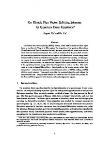
For the transonic computations presented below, we take a GaAs diode of length L = 0.75 µm at T0 = 300 K as shown in Figure 1. The applied voltage Vb = 1.5 V . The length of the device is divided as 0.25 µm source (n+ ), 0.25 µm channel (n) and 0.25 µm drain (n+ ). Moreover the physical parameters are the effective electron mass m = 0.0631 me at 300 K, where me is the electron mass and the dielectric constant ε = 12.9. We considered the constant relaxation times i.e. τp = τw = 0.2 picoseconds. Because of subsonic inflow and outflow, we set the boundary conditions on the left as n = C(x), T = T0 , V = 0 and on the right as n = C(x) and V = 1. The numerical results for physical variables are displayed in Figure 2 on 200 grid points. It can be observed from the plots that the proposed KFVS scheme has better ability to resolve steep fronts appeared in the velocity and temperature profiles as compared to the NT central splitting scheme. Secondly, we simulate an n+ − n − n+ ballistic silicon diode with an applied voltage Vb = 1.5V . The domain of semiconductor is defined on the [0, L] with L = 0.6 µm. The source region is of 0.1 µm, the channel length is of 0.4 µm and the drain region is of 0.1 µm. The doping profile is

C(x) =

  2 × 1021 m−3 ,

x ∈ (0.1µm, 0.5µm),

 5 × 1023 m−3 ,

elsewhere.

(53)

Further, the physical parameters required in the simulations are listed in the Table 1. Figure 3 compares the results of KFVS and NT central schemes on 200 grid points (∆x = 3.0 × 10−3 µm). The electric field and considered initial conditions contributed 16

in the oscillations during the first few picoseconds. Afterwards, the solution tends to a steady state condition. From the Figure 3, it can be observed that both the KFVS and the NT central schemes give comparable results. A small overshoot can be observed in the results of KFVS and NT central schemes at end of channel length in the velocity profile. KFVS resolves that peak more accurately as compared to the NT central scheme. Overall, the results of both schemes agree well. Similar results and peaks were also obtained in literature, see for example [27] and references therein.

Thirdly, we make a numerical convergence study of our proposed numerical scheme. In Figure 4, the results of KFVS scheme on different grid points are displayed, i.e. on 50 grid points (∆x = 1.2 × 10−2 µm), 100 grid points (∆x = 6.0 × 10−3 µm), 200 grid points (∆x = 3.0 × 10−3 µm), and 400 grid points (∆x = 1.5 × 10−3 µm).

Minor differences in the concentration and energy density profiles can be observed throughout the diode. In velocity and electric field profiles differences are clear in source and drain region. The velocity overshoot in the second junction clearly becomes sharper with finer grids. These are known effects of the numerical viscosity. Small viscosity is taken in account for finer mesh. This is the fact that around the places having discontinuities and heavy gradients, the numerical solution faded out. Comparatively small difference can be seen in the temperature only in drain region. This can be explained by analyzing the steady states. The difference in u is reflected in n reciprocally. Because n ranges from around 10 to 500, this difference is barely observable. The difference in n interferes the electric field through the Poisson equation.

Let us make a quantitative analysis of the differences. The reference solution is obtained from the KFVS on 800 grid points. The L1 and L∞ errors are given in Table 2 on different grid points. The numerical convergence rates for the L1 error are also computed. The units of the L∞ and L1 errors are the same as the corresponding quantities. As we have mentioned earlier around the second junction the large gradients (discontinuities) occurs. This is the 17

point where most of the hyperbolic solver can only ensures first order accuracy. Similar accuracy was obtained by our proposed numerical scheme. Similarly, L∞ -error cannot be neglected around the second junction. Whereas, the L∞ -error rapidly reduces away from this junction. We also conclude that the spike may be involved with a numerical artifact similar to that in a slowly moving discontinuity [28]. The L1 -error converges between 1 and 2 as the our proposed numerical scheme loses the second order accuracy around the discontinuities. For comprehensive overview of L∞ and L1 -errors are displayed in Figure 5. 4.1.2. The effects of different mobilities, temperatures and channel lengths The use of different physical parameters in the hydrodynamical model changes its solution. Such effects were also analyzed in the literature, see for example [30, 31] and references therein. We also analyzed the same behaviors through our proposed numerical algorithm. For this purpose, different numerical solutions were obtained with different mobilities µn , different lattice temperatures T0 and different channel lengths. Figure 6 shows that different values of mobilities produce no considerable changes in the density n. Whereas, the humps and peaks of velocity u and energy E decreases on decreasing the mobility constant. Moreover, a decrease in mobility constant flattered the temperature T .

In Figure 7 displays the effects of different lattice temperatures on the solutions. It can be seen that there no much difference in the density profile. However, the peak of velocity u and range of energy E reduces with reducing the temperature T0 . It can be observed in Figure 8 that with smaller channel length there is no diminishing behavior of hump is seen in the velocity profile u. Similarly, flatness is no more prominent in the temperature profile T .

18

The observations of Figures (6)-(8) were also reported in [30, 31]. 4.1.3. The effect of the different voltage In this test problem, we have simulated n+ − n − n+ ballistic silicon diode with an applied voltage Vb = 2.0V . However, the doping profile is same as defined in Eq. (53). It can be seen from the Figure 9 that our proposed numerical scheme gives almost the same result as obtained from NT central scheme. We have also plotted the electric potential V calculated from the Poisson equation (c.f. Eq. (4)). 4.1.4. The effect of the different physical parameters In this test problem, we considered a semiconductor of length L = 0.8 µm with a source region of 0.175 µm, channel length of 0.45 µm and drain region of 0.175 µm. The doping profile is

C(x) =

  2 × 1021 m−3 , x ∈ (0.175µm, 0.45µm),  5 × 1023 m−3 ,

(54)

elsewhere.

However, we have changed the effective electron mass to m∗ = 0.065 × 0.9190 × 10.0−31 kg, permittivity constant to εs = 13.2×8.85418×10−12 F/m and low field mobility constant to µn = 0.14m2 /Vs . From the Figure 10, it can be observed that the KFVS has comparative results with the NT central scheme. 4.2. Two dimensional test problems Now, we simulate the two-dimensional problem for the validation of the proposed scheme. We present the numerical simulation of 2D MESFET device of size 0.6 × 0.2µm2 , with HD model. The source and the drain each occupies 0.1µm. The source is at x ∈ [0, 0.1] and y = 0.2 and the drain is at x ∈ [0.5, 0.6] and y = 0.2. The gate occupies 0.2µm at x ∈ [0.2, 0.4] and y = 0.2. The doping is defined by nd = 3×1017 cm−3 in [0, 0.1]×[0.15, 0.2] and in [0.5, 0.6] × [0.15, 0.2] and nd = 1 × 1017 cm−3 elsewhere, with abrupt junction (see

19

Figure. 11).

We apply, at the source and drain, a voltage bias vbias = 2V and at the gate negative bias voltage = −0.8V and low concentration n = 3.9 × 105 cm−3 . The numerical boundary conditions are summarized as: Ô

At the source (0 ≤ x ≤ 0.1, y = 0.2): φ = φ0 for the potential; n = 3 × 1017 cm−3 for

the concentration; T = 300o for the temperature; v1 = 0µm/ps for the horizontal velocity; and the Neumann boundary conditions for the vertical velocity v2 . Ô

At the drain (0.5 ≤ x ≤ 0.6, y = 0.2): φ = φ0 + 2 for the potential; n = 3 × 1017 cm−3

for the concentration; T = 300o for the temperature; v1 = 0µm/ps for the horizontal velocity; and the Neumann boundary conditions for the vertical velocity v2 . Ô

At the gate (0.2 ≤ x ≤ 0.4, y = 0.2): φ = φ0 −0.8 for the potential; n = 3.9×105 cm−3

for the concentration; T = 300o for the temperature; v1 = 0µm/ps for the horizontal velocity; and the Neumann boundary conditions for the vertical velocity v2 . Ô

At all other parts of the boundary, all variables equipped with the Neumann boundary

conditions. In Figure 12, the surface plots for the density n, the temperature T , the horizontal velocity v1 , the vertical velocity v2 and the potential φ obtained by KFVS scheme with 96 × 32 uniform mesh points are presented. It can be seen that final steady solution has several singularities/sharp transitions due to jumps in the doping nd and the mixed DrichletNewmann boundary conditions. In Figure 13, a comparison of cuts at y = 0.175 of the solution is shown, between KFVS and central scheme with 92 × 32 uniform meshes. The KFVS scheme shows better results in capturing sharp peaks and NT central produces diffusive results 5. Conclusions A second order accurate splitting scheme based on the KFVS method was presented to solve the multi dimensional hydrodynamical models describing charge transport in semiconductor devices. The nonlinear transport processes, high gradients and stiff relaxation 20

parameters in the models were the main sources of instabilities for a numerical scheme. For comparison and validation, a splitting scheme based on the NT central scheme was also applied to the same model. It was found that the suggested KFVS method has capability to capture narrow peaks and steep gradients in the solution profiles. Further, the solutions of proposed scheme were free of oscillations. This was demonstrated by considering the case studies of several one-dimensional n+ − n − n+ diodes. Moreover, the numerical solution obtained with different temperatures, mobilities and voltages further validated the robustness and efficiency of the current method. A two dimensional simulation is also performed by KFVS method for a MESFET device, producing results in good agreement with those obtained by NT-central scheme.

21

References [1] N. Tessler, Y. Roichman. Two-dimensional simulation of polymer field-effect transistor. Appl. Phys. 79 (2001) 2987-2989. [2] M. Gharghi, H. Bai, G. Stevens, S. Sivoththaman. Three-dimensional modeling and simulation of pn junction spherical silicon solar cells. IEEE Trans. Electron Devices. 53 (2006) 55-63. [3] D. Alexei, J. Sajeev. Finite difference discretization of semiconductor drift-diffusion equations for nanowire solar cells. Comput. Phys. Com. 183 (2012) 28-35. [4] C. Jacoboni, P. Lugli. The Monte Carlo Method for Semiconductor Device Simulation. Wien Springer. (1989). [5] P. A. Markowich, C. A. Ringhofer, C. Schmeiser, Semiconductor Equations, Springer, Berlin. 4 (1990) 248 pages. [6] S. Selberherr, Analysis and Simulation of Semiconductor Devices, Springer, Berlin. 1 (1984). [7] K. Blotekjar, Transport equations for electrons in two-valley semiconductors, IEEE Trans. Electr. Dev. 17 (1970) 38-47. [8] G. Baccarani, M. Wordeman, An investigation on steady-state velocity overshoot in silicon, Solid-State Electr. 29 (1982) 970-977. [9] M. Rudan, F. Odeh, Multi-dimensional discretization scheme for the hydrodynamic model of semiconductor devices, COMPEL. 5 (1986) 149-183. [10] C. Bardos, F. Golse, and C.D. Levermore, Fluid dynamical limits of kinetic equations. I. Formal derivations, J. Stat. Phys. 63 (1991) 323-344. [11] C. Gardner, Numerical simulation of a steady-state electron shock wave in a submicron semiconductor device, IEEE Trans. Electr. Dev. 38 (1991) 392-398. 22

[12] X. Jiang, A streamline-upwinding/PetrovGalerkin method for the hydrodynamic semiconductor device model, Math. Models Meth. Appl. Sci. 5 (1995) 659-681. [13] Z. Chen, B. Cockburn, J. Jerome, C.-W. Shu, Mixed-RKDG finite element methods for the 2-D hydrodynamic model for semiconductor device simulation, VLSI Des. 3 (1995) 145-158. [14] J. Jerome, C.-W. Shu, Energy models for one-carrier transport in semiconductor devices, in: W. Coughran, J. Colde, P. Lloyd, J. White (Eds.), Semiconductors, Part II, in: IMA Vol. in Math. Appl. 59 (1994) 185-207. [15] C. W. Shu, Essentially non-oscillatory and weighted essentially non-oscillatory schemes for hyperbolic conservation laws, ICASE Report No. 97-65, NASA Langley Research Center, Hampton, VA. (1997). [16] V. Romano, G. Russo, Numerical solution for hydrodynamic models of semiconductors, Preprint, Universita dellAquila, Italy. 7 (2000) 1099-1120. [17] M. Anile, V. Romano, G. Russo, Extended hydrodynamic model of carrier transport in semiconductors, SIAM J. Appl. Math. 61 (2000) 74-101. [18] J. C. Mandal and S. M. Deshpande. Kinetic Flux-Vector Splitting for Euler Equations. Computer and Fluids. 23 (1994) 447-478. [19] B. Van Leer. Flux Vector Splitting for the Euler Equations. ICASE. (1982), Report No. 82-30. [20] A. Harten, P. D. Lax and B. Van Leer. On Upstream Differencing and Godunov-Type Schemes for Hyperbolic Conservation Laws. SIAM Review. 25 (1983) 35-62. [21] N. P. Weatherill, J. S. Mathur and M. J. Marchant. An Upwind Kinetic Flux Vector Splitting Method on General Mesh Topologies. Int. J. Numer. Meth. Eng. 37 (1994) 623-643.

23

[22] K. Xu. Gas-Kinetic Theory Based Flux Slitting Method for Ideal MagnetoHydrodynamics. J. Comput. Phys. 153 (1999) 334-352. [23] T. Tang and K. Xu. A High-Order Gas-Kinetic Method for Multidimensional Ideal Magnetohydrodynamics. J. Comput. Phys. 165 (2000) 69-88. [24] H. Tang, T. Tang and K. Xu. A Gas-Kinetic Scheme for Shallow-Water Equations with Source Terms. Z. Mathe. Phys. 55 (2004) 365-382. [25] K. Xu. A Well-Balanced Gas-Kinetic Scheme for the Shallow-Water Equations with Source Terms. J. Comput. Phys. 178 (2002) 533-562. [26] C. W. Shu, S. Osher, Efficient Implementation of Essentially Non-Oscillatory Shock Capturing Schemes. J. Comput. Phys. 77 (1988) 439-471. [27] S, Zia, M. Ahmed and S. Qamar. A Gas-Kinetic Scheme for Six-Equation Two-Phase Flow Model. Appl. Math. 5 (2014) 453-465. [28] S. Jin, J. Liu, The effects of numerical viscosities I: slowly moving shocks, J. Comput. Phys. 126 (1996) 373-389. [29] G. S. Jaing, E. Tadmor, Non-oscillatory central schemes for multidimensional hyperbolic conservation laws. SIAM J. Sci. Comput. 19 (1998) 1892-1917. [30] A. Jungel and S. Tang. A discrite BGK approximation for the hydrodynamic equations for semiconductors. Appl. Numer. Math. (2001). [31] A. Jungel and S. Tang. A relaxation scheme for the hydrodynamic equations for semiconductors. Appl. Numer. Math. 43 (2002) 229-252.

24

Table 1: Physical parameters.

Parameter

Physical meaning

Numerical values

q

elementary charge

1.6 × 10−19 C

m∗

effective electron mass

0.26 × 9.11 × 10−31 kg

εs

permittivity constant

11.7 × 8.85 × 10−12 F/m

µn

low field mobility constant

0.1 m2 /Vs

kB

Boltzman constant

1.38 × 10−23 J/K

T0

lattice temperature

300 K

ni

intrinsic electron concentration

1.4 × 1016 m3

vs

saturation velocity

1.03 × 105 m/s

Figure 1: n+ − n − n+ Diode with channel lenght 0.75µm and Vb = 1.5V

. 5.1. One-dimensional KFVS method In this sub-section, we implement the KFVS scheme on the system of Eqs. (15) and then solve it. In the gas-kinetic theory, the motion of particle between cell interfaces is explained by the term flux. The evaluation of local macroscopic flux-vector F (W ) will be accomplished by the numerical discretization of the current system across complete 25

Table 2: Numerical errors for different number of grid points.

Grid Numbers

Density (n)

Velocity (u)

L∞

L1

rate

L∞

L1

rate

50

4.84

36.63

-

0.030

0.23

-

100

2.30

11.06

1.73

0.013

0.08

1.52

200

0.35

3.84

1.53

0.002

0.019

2.07

400

0.15

1.11

1.79 0.0007

0.007

1.44

Grid Numbers

Temperature (T)

Electric field (-Vx )

L∞

L1

rate

L∞

L1

rate

50

0.0439

0.165

-

0.083

0.65

-

100

0.0090

0.053

1.64

0.056

0.21

1.63

200

0.0016

0.018

1.56

0.007

0.073

1.52

400

0.0002

0.005

1.85

0.002

0.014

2.38

Grid Numbers

Energy (E) L∞

L1

rate

50

4.58

40.98

-

100

2.11

11.50

1.83

200

0.31

4.11

1.48

400

0.11

1.05

1.97

26

600 KFVS

KFVS

1.6

CENTRAL

CENTRAL

500 1.4 1.2

Velocity (u)

Density (n)

400

300

1 0.8 0.6

200

0.4 100 0.2 0

−2

−1

0

1

2

3

4

0

5

−2

−1

0

1

x−axis

2

3

4

5

3

4

5

x−axis

350

0.5 KFVS CENTRAL

300

KFVS

0.45

CENTRAL

0.4

Temperature (T)

200

150

0.35 0.3 0.25 0.2 0.15

100 0.1 0.05

50

0 0

−2

−1

0

1

2

3

4

5

−2

−1

0

1

2

x−axis

x−axis

4 KFVS CENTRAL

2 0

Electric field (−Vx)

Energy (E)

250

−2 −4 −6 −8 −10 −12 −14

−2

−1

0

1

2

3

4

5

x−axis

Figure 2: Comparison: KFVS vs Central (∆x = 3.0 × 10−3 µm).

27

600

2 KFVS CENTRAL

500

1.4

Velocity (u)

Density (n)

CENTRAL

1.6

400

300 403.6 403.4

200

403

100

1.2 1 0.8

1.19 1.185

0.6

403.2

1.18

0.4

1.175 5.155

0

KFVS

1.8

0

1

5.16

2

5.165

0.2

3

4

5

0

6

4.42 0

1

2

4.46

3

x−axis

4

5

6

5

6

x−axis

400

2 KFVS

KFVS 350

1.8

CENTRAL

CENTRAL

1.6

Temperature (T)

300 250 200 152 150

151

1.4 1.2 1 0.8

1.48

0.6

1.46

150

100

5.02

5.04

5.06

50

0.4

0

0.2

1

2

3

4

5

6

1.44 3.9 0

1

2

3

x−axis

4 4

x−axis

4 KFVS CENTRAL 2

x

0

Electric field (−V )

Energy (E)

4.44

0

−2

−4 −1.664 −1.666 −6

−1.668 1.906

−8

0

1

1.908 2

3

4

5

6

x−axis

Figure 3: Comparison: KFVS vs Central with 200 grid points (∆x = 3.0 × 10−3 µm).

28

600 2

50−Grids

50−Grids 100−Grids

100−Grids 500

200−Grids

200−Grids 400−Grids

400−Grids

1.5

Velocity (u)

Density (n)

400

300 198 200

197

1

1.02 0.5

1.01

196

1

195

100

0.99

194 0

0

1

0.98

0 1

2

1.05 3

4.9 4

5

6

1

2

x−axis

4

5

6

x−axis

400

1.8 50−Grids

50−Grids 100−Grids

350

100−Grids

1.6

200−Grids

200−Grids 400−Grids

250 332

200

331 150 330 100

400−Grids

1.4

Temperature (T)

300

1.2 1 0.8 1.76 0.6

329

1.74 5.16

50

5.18

5.2

0.4 1.72

0

1

2

3

4

5

0.2

6

0

1

2

3

x−axis

4.45 4.5 4.55 4

x−axis

4 50−Grids 100−Grids 2

200−Grids 400−Grids

x

0

Electric field (−V )

Energy (E)

4.95 3

0

−2

−4

−5.4 −5.5

−6

−5.6 −8

5 0

1

5.05

5.1 2

3

4

5

6

x−axis

Figure 4: Numerical solutions with successive double grid points.

29

5

6

L1 ERROR

2

10

Density (n) Velocity (u) Temperature (T) Electric field (−Vx)

1

10

Energy (E)

0

10

−1

10

−2

10

50

100

150

200

250

300

350

400

Number of Grid Points

L∞ ERROR 1

Density (n) Velocity (u) Temperature (T) Electric field (−Vx)

10

0

10

Energy (E) −1

10

−2

10

−3

10

−4

10

50

100

150

200

250

300

350

400

Number of Grid Points

Figure 5: Convergence Study of the Scheme.

boundary of the mesh cell. Flux function can be determined by the motion of particle in the x-direction. The other quantities, like densities, pressure and energy can be treated as passive scalars moving with the particles velocity. Commonly, particles are distributed randomly around the average velocity. In statistical mechanics, the local Maxwellian distribution function explains the motion of moving particles across coordinate directions. The normal direction n for the Maxwellian distribution function fM is given as (e.g. [25]) µ ¶ 12 λ fM (t, n, vn ) = n exp[−λ(unˆ − vnˆ )2 ], π

λ=

m∗ 2kB T0

(55)

where n, m∗ , kB and T0 are density, effective electron mass, Boltzmann constant and lattice 30

temperature respectively. The transport of any flow quantity is due to the movement of particles. Thus, in the one-dimensional case, with the distribution function fM given by Eq. (55) the particles can be divided into two groups. First group is moving with the positive velocity (un > 0) in the right direction (un > 0) and the second group is moving with the negative velocity (un < 0) in the left direction. Let us defined the moments, these moments will be sufficient enough for splitting the fluxes, µ ¶ 12 λ 2 hv inˆ = 1 = e−λ(unˆ −vnˆ ) dvnˆ , π −∞ Z ∞ µ ¶ 12 λ 2 hv 1 inˆ = unˆ = vnˆ e−λ(unˆ −vnˆ ) dvnˆ . π −∞ Z

0

∞

(56) (57)

The zeroth order moment in Eq. (56) is used to split scalars, while the first order moment in Eq. (57) is used for splitting vectors. In order to simplify the notation, we define µ ¶ 12 √ λ 1 2 = e−λ(unˆ −vnˆ ) dvnˆ = erf c(− λunˆ ), π 2 0 Z 0 µ ¶ 12 √ λ 1 2 = e−λ(unˆ −vnˆ ) dvnˆ = erf c( λunˆ ), π 2 −∞ Z

hv 0 i+ˆn hv 0 i−ˆn

∞

(58) (59)

and µ ¶ 12 2 λ 1 e−λunˆ 2 −λ(un 0 ˆ −vn ˆ) = vnˆ e dvnˆ = unˆ hv i+ˆn + √ , π 2 πλ 0 Z 0 µ ¶ 12 2 λ 1 e−λunˆ 2 −λ(un 0 ˆ −vn ˆ) = vnˆ e dvnˆ = unˆ hv i−ˆn − √ , π 2 πλ −∞ Z

hv 1 i+ˆn hv 1 i−ˆn

∞

(60) (61)

In the above equations, the motion of the particles in the right direction is represented by the positive sign and the motion of the particles in the left direction is represented by the negative sign. Moreover, the complementary error function is defined as Z ∞ 2 2 erf c(z) = √ e−t dt. π z

(62)

Now the Eq. (15) can be solved by KFVS scheme with thr help of above mentioned flux splitting technique. For the implementation of finite volume scheme, first we sub-divide the domain into N sub domains. Let us define the cell Ii by interval [xi− 1 , xi+ 1 ] for 2

31

2

i = 1, 2, · · · , N . Therefore, ∆x = xi+ 1 − xi− 1 represents the uniform cells width, the 2

2

points xi = i∆x refer to the cells center and the points xi± 1 = xi ± ∆x/2 represent the 2

cells faces. We start with a cell averaged initial data

Win

at time step tn and compute the

cell average updated solution Win+1 over the same cells at the next time step tn+1 . With the help of above defined setup we can split the flux function in Eq. (15) as   nu     2 F (W ) ==  nu + P  = F + + F − ,   u(E + P )

(63)

where  F

±

  = hv i±x   1





n

 0

    0  + hv i±x  P nu   1 u(E + 12 P ) Pu 2

  . 

(64)

Here, the right interface flux vector of the cell Ii is defined as − Fi± 1 = Fi+ + Fi+1 . 2

(65)

Similarly, the left interface flux vector of the cell Ii . The integration of the Eq. (7) over the cell [xi− 1 , xi+ 1 ] gives the following semi-discrete kinetic upwind scheme 2

2

Fi+ 1 − Fi− 1 dWi 2 2 =− . dt ∆x

(66)

The cell averaged values Wi are defined as 1 Wi := Wi (t) = ∆x

Z

xi+ 1 2

W (t, x)dx.

(67)

xi− 1 2

The above scheme has first order accuracy in space. However, the high order accuracy can be achieved. For this the initial reconstruction procedure will be applied for interpolating the cell averaged variables Wi . In this article, a second order accurate MUSCL-type initial reconstruction strategy is used. Setting Wi be the piecewise constant solution. Furthermore, selection of the slope vector (differences) Wx in the x-direction help us in 32

the reconstruction of a piecewise linear (MUSCL-type) approximation. The boundary extrapolated values are given as 1 WiL = Wi − Wix , 2

1 WiR = Wi − Wix . 2

(68)

A possible computation of these slopes, is given by family of discrete derivatives parameterized with 1 ≤ θ ≤ 2, for example ½ µ ¶ ¾ θ x Wi = M M θ∆Wi+ 1 , ∆Wi+ 1 + ∆Wi− 1 , θ∆Wi− 1 , 2 2 2 2 2

(69)

where 1 ≤ θ ≤ 2 is a parameter and ∆ denotes the central differencing ∆Wi+ 1 = Wi+1 − Wi . 2

Here, M M denotes the min-mod non-linear limiter     min{xi } if xi > 0 ∀i,    i M M {x1 , x2 , ...} = max{xi } if xi < 0 ∀i,  i     0 otherwise.

(70)

(71)

On the basis of above reconstruction procedure, a semi-discrete high resolution kinetic solver is given as L R Fi+ 1 (Wi+1 , WiR ) − Fi− 1 (WiL , Wi−1 ) dWi 2 2 =− . dt ∆x

(72)

A second order TVD Runge-Kutta scheme is used to solve Eq. (72). Let the right hand side of Eq. (72) as L(W ), two stages will be require for updating W using second order TVD Runge-Kutta scheme [22] W

(1)

n

n

= W + ∆tL(W ) ,

W

(n+1)

µ ¶ 1 n (1) (1) = W + W + ∆tL(W ) , 2

(73)

where W n is solution at the previous time step and W n+1 is updated solution at the next time step. Moreover, ∆t represents the time step.

33

600

2 2

µn=0.1 m2/Vs

µn=0.08 m2/Vs

2

µn=0.08 m /Vs

500

1.6

2

µn=0.06 m /Vs

µn=0.06 m2/Vs

1.4

2

µ =0.04 m /Vs

400

n

Velocity (u)

Density (n)

µn=0.1 m /Vs

1.8

300

200

µn=0.04 m2/Vs

1.2 1 0.8 0.6 0.4

100

0.2 0

0

1

2

3

4

5

0

6

0

1

2

3

x−axis

400

6

4

5

6

2

µn=0.08 m /Vs µn=0.06 m2/Vs

Temperature (T)

µn=0.04 m /Vs

200 150

0.8

50

0.4

3

4

5

0.2

6

0

1

2

3

x−axis

x−axis

4 µn=0.1 m2/Vs µn=0.08 m2/Vs

2

x

Electric field (−V )

2

µn=0.04 m2/Vs

1

0.6

1

µn=0.06 m2/Vs

1.2

100

0

µn=0.08 m2/Vs

1.4

2

250

µn=0.1 m /Vs

1.6

2

300

Energy (E)

5

1.8 µn=0.1 m2/Vs

350

0

4

x−axis

µn=0.06 m2/Vs 2

µn=0.04 m /Vs

0

−2

−4

−6

−8

0

1

2

3

4

5

6

x−axis

Figure 6: Numerical solutions for different low field mobility.

34

600

2 T =300 K 0

T0=100 K

1.6

T =100 K

T0=80 K

1.4

T =80 K

0

Velocity (u)

400

Density (n)

T0=200 K

T0=200 K

500

T0=300 K

1.8

300

200

0

1.2 1 0.8 0.6 0.4

100

0.2 0

0

1

2

3

4

5

0

6

0

1

2

3

x−axis

400 350

6

4

5

6

T0=300 K

1.6

T0=200 K T0=100 K

300

T0=200 K T0=100 K

1.4

Temperature (T)

T0=80 K

250 200 150 100

T0=80 K 1.2 1 0.8 0.6 0.4

50

0.2

1

2

3

4

5

0

6

0

1

2

3

x−axis

x−axis

4 T0=300 K T0=200 K

2

T0=100 K

x

0

Electric field (−V )

Energy (E)

5

1.8 T0=300 K

0

4

x−axis

T0=80 K

0

−2

−4

−6

−8

0

1

2

3

4

5

6

x−axis

Figure 7: Numerical solutions for different lattice temperatures.

35

500

µn=0.1 m2/Vs

0.9 2

µn=0.1 m /Vs

450

µ =0.08 m /Vs 2

µn=0.06 m /Vs µn=0.03 m2/Vs

350

µn=0.03 m2/Vs

0.7

Velocity (u)

Density (n)

µn=0.06 m2/Vs

n

400

300 250

0.6 0.5 0.4

200

0.3

150

0.2

100

µn=0.08 m2/Vs

0.8

2

0

0.5

1

1.5

2

0.1

2.5

0

0.5

1

x−axis

1.5

2

2.5

1.5

2

2.5

x−axis

350 µn=0.1 m2/Vs µn=0.08 m2/Vs

0.55

300 2

µn=0.1 m /Vs

Temperature (T)

µn=0.08 m /Vs

250

µn=0.06 m2/Vs µn=0.03 m2/Vs

200

150

0.5

µn=0.03 m2/Vs

0.45

0.4

0.35 100 0.3 50

0

0.5

1

1.5

2

2.5

0

0.5

1

x−axis

x−axis

−2 −4 2

µn=0.1 m /Vs

−6

Electric field (−Vx)

Energy (E)

µn=0.06 m2/Vs

2

µn=0.08 m2/Vs

−8

µn=0.06 m2/Vs µn=0.03 m2/Vs

−10 −12 −14 −16 −18 −20

0

0.5

1

1.5

2

2.5

x−axis

Figure 8: Numerical solutions for different low field mobility for channel length 50nm.

36

600

2 KFVS

KFVS 1.8

CENTRAL 500

CENTRAL

1.6 1.4

Velocity (u)

Density (n)

400

300

200

100

0

1

1 0.8

480

0.6

0.6

478

0.4

0.58

476

0.2

0.56

0.8 0

1.2

2

0.82 0.84 3

0 4

5

6

1.2 0

1

1.25

2

x−axis

4

6

5

6

2.5 KFVS

400

KFVS

CENTRAL

CENTRAL 2

Temperature (T)

350 300 250 400 200

395

150

390

100

385 5.3

5.4

1.5

1 2.3 2.25

0.5

5.5

2.2

50

4.6 0

5

x−axis

450

Energy (E)

1.3

3

0

1

2

3

4

5

0

6

0

1

2

x−axis

4.8

3

4

x−axis

4 2.4

KFVS CENTRAL

2

KFVS CENTRAL

2.2

Electric potential (V)

Electric field (−Vx)

2 0

−2

−4 1.904

−6

1.902 −8

1.8 1.6 1.4 1.2 0.54 1 0.52

0.8

1.9

0.6 0.5

−10

1.066 1.067 1.068 0

1

2

0.4 3

4

5

6

1

x−axis

2

3

2.1 4

2.15 5

2.2 6

x−axis

Figure 9: Comparison: KFVS vs Central with an applied Voltage Vb = 2.0V (∆x = 3.0 × 10−3 µm).

37

1200

2.5 KFVS

KFVS

CENTRAL

CENTRAL

800

1.5

Velocity (u)

2

Density (n)

1000

600

1 2.05

862

400

0.5 2

860 200

0 1.95 858 6.38

0

0

1

2

3

6.4

4

5

5.8 6

7

−0.5

8

0

1

2

3

x−axis

6 4

5

6

7

8

6

7

8

x−axis

800

2.5 KFVS

KFVS

CENTRAL

700

CENTRAL 2

Temperature (T)

500 400 536

300

534 200

532

1 2.05 2

0.5 6.3

0

1

2

3

1.95 5.435 5.44 5.445

6.35 4

5

6

7

0

8

0

1

2

3

x−axis

4

5

x−axis

6 KFVS CENTRAL

4

x

0

1.5

530

100

Electric field (−V )

Energy (E)

600

2

0

−2 1.1 −4 1.08 −6

−8

1.06

0

1

1.93 1.94 1.95 2 3

4

5

6

7

8

x−axis

Figure 10: Comparison: KFVS vs Central (∆x = 4.0 × 10−3 µm).

38

23

x 10 3

Density (n)

2.5 2 1.5 1 0.5 0 2 1.5 −7

x 10

6 1

4 0.5

y−axis

−7

2 0

0

x 10

x−axis

Figure 11: 2D doping nd = (1012 cm−3 ) in [0, 0.6] × [0, 0.2] (µm2 )

39

22

5

x 10

x 10

Horizontal Velocity (v1)

3.5

Density (n)

3 2.5 2 1.5 1 0.5 2

5

0

−5

2 1.5 1

−7

x 10

0.5

2

1

y−axis

4

3

5

6

1.5 1

−7

x 10

−7

0.5

x 10

1

2

y−axis

x−axis

3

4

5

6 −7

x 10

x−axis

5

x 10

3500 Temperature (T)

Vertical Velocity (v2)

0 −2 −4 −6 −8 −10

3000 2500 2000 1500 1000 500

2

2 1.5

−7

x 10

1 0.5

3

2

1

y−axis

4

5

6

1.5 1

−7

x 10

−7

0.5

x 10

1

y−axis

x−axis

2

3

4

5

6 −7

x 10

x−axis

2.5 2

Vx

1.5 1 0.5 0 −0.5 2 1.5 −7

x 10

6 1

4 0.5

y−axis

−7

2 0

0

x 10 x−axis

Figure 12: 2D MESFET, HD model. Top left: Density (n), Top right: Horizontal velocity (v1 ), middle left: Vertical velocity (v2 ), middle right: Temperature(T ), bottom: Electric Potential (Vx ).

40

5

22

x 10

x 10

8 KFVS CENTRAL

3.5

KFVS CENTRAL

6 4

Density (n)

1

Horizontal Velocity (v )

3

2.5

2

1.5

1

2 0 −2 −4 −6 −8

1

2

3

4

5

x−axis

6

1

2

3

4

5

x−axis

−7

x 10

6 −7

x 10

5

0.5

x 10

KFVS CENTRAL

0

KFVS CENTRAL

3500

−0.5 3000

Temperature (T)

Vertical Velocity (v2)

−1 −1.5 −2 −2.5 −3

2500

2000

1500

−3.5 1000

−4 −4.5 1

2

3 x−axis

4

5

6

1

2

3

x−axis

−7

x 10

4

5

6 −7

x 10

KFVS CENTRAL

2.5

Electric Field (EF)

2

1.5

1

0.5

0 1

2

3

x−axis

4

5

6 −7

x 10

Figure 13: 2D MESFET, HD model. Cut at y = 0.175. Top left: Density (n), Top right: Horizontal velocity (v1 ), middle left: Vertical velocity (v2 ), middle left: Temperature(T ), bottom: Electric Potential (Vx ).

41