Chapman University
Chapman University Digital Commons Psychology Faculty Articles and Research
Psychology
12-7-2017
Application of Real Field Connected Vehicle Data for Aggressive Driving Identification on Horizontal Curves Arash Jahangiri San Diego State University
Vincent Berardi Chapman University,
[email protected]
Sahar Ghanipoor Machiani San Diego State University
Follow this and additional works at: https://digitalcommons.chapman.edu/psychology_articles Part of the Automotive Engineering Commons, Controls and Control Theory Commons, Other Electrical and Computer Engineering Commons, Other Operations Research, Systems Engineering and Industrial Engineering Commons, Risk Analysis Commons, Systems and Communications Commons, and the Transportation Engineering Commons Recommended Citation Jahangiri, A., Berardi, V., & Machiani, S. G. (2017). Application of real field connected vehicle data for aggressive driving identification on horizontal curves. IEEE Transactions on Intelliginet Transportations Systems, 19(7). doi: 10.1109/TITS.2017.2768527
This Article is brought to you for free and open access by the Psychology at Chapman University Digital Commons. It has been accepted for inclusion in Psychology Faculty Articles and Research by an authorized administrator of Chapman University Digital Commons. For more information, please contact
[email protected].
Application of Real Field Connected Vehicle Data for Aggressive Driving Identification on Horizontal Curves Comments
This is a pre-copy-editing, author-produced PDF of an article accepted for publication in IEEE Transactions on Intelliginet Transportations Systems in 2017 following peer review. The definitive publisher-authenticated version is available online at DOI: 10.1109/TITS.2017.2768527. Copyright
IEEE
This article is available at Chapman University Digital Commons: https://digitalcommons.chapman.edu/psychology_articles/110
T-ITS-17-06-0533.R1
1
Application of Real Field Connected Vehicle Data for Aggressive Driving Identification on Horizontal Curves Arash Jahangiri, Vincent Berardi, and Sahar Ghanipoor Machiani
Abstract—The emerging technology of connected vehicles generates a vast amount of data that could be used to enhance roadway safety. In this study, we focused on safety applications of a real field connected vehicle data on a horizontal curve. The database contains connected vehicle data with instrumented vehicles that were carried out on public roads in Ann Arbor, Michigan. Horizontal curve negotiations are associated with a great number of accidents, which are mainly attributed to driving errors. Aggressive/risky driving is a contributing factor to the high rate of crashes on horizontal curves. Using basic safety message (BSM) data in connected vehicle dataset, this study modeled aggressive/risky driving while negotiating a horizontal curve. The model was developed using the machine learning method of Random Forest to classify the value of time to lane crossing (TLC), a proxy for aggressive/risky driving, based on a set of motion-related metrics as features. Three scenarios were investigated considering different TLCs value for tagging aggressive driving moments. The model contributed to high detection accuracy in all three scenarios. This suggests that the motion-related variables used in the random forest model can accurately reflect drivers’ instantaneous decisions and identify their aggressive driving behavior. The results of this study inform the design of warning/feedback systems and control assistance from unsafe events which are transmittable through vehicles-to-vehicles (V2V) and vehicles-to-infrastructure (V2I) applications. Index Terms— Aggressive driving, connected vehicle data, horizontal curves, random forest, traffic safety
I. INTRODUCTION
W
ith the advent of connected vehicles (CV) technology, there will be an unprecedented opportunity for applications of vehicles-to-vehicles (V2V) and vehicles-toinfrastructure (V2I) communications. Applications of CV technology focus on four main objectives: improving safety, A. Jahangiri (corresponding author) is a Research Faculty with the Department of Civil, Construction, and Environmental Engineering, San Diego State University, San Diego, 5500 Campanile Dr., CA 92182 USA (e-mail:
[email protected]). V. Berardi is an Assistant Professor with the Department of Psychology, Chapman University, 1 University Dr, Orange, CA 92866 USA (e-mail:
[email protected]).
enhancing mobility, improving operational performance, and reducing environmental impacts. Focusing on safety applications such as work zone alerts, stop sign violation warnings, and curve speed warnings [1], it is expected that V2V communication systems could potentially address approximately 80% of all police-reported crashes annually [2]. Soon, as the technology becomes more available, affordable, and acceptable by the public, it will be implemented in an increasing number of vehicles, providing a large volume of data. Intelligence obtained from such “big data” has the potential to enhance safety by providing immediate feedback to drivers as well as informing advanced driver-assistance systems. Research on CV technology and applications is a relatively new area of study. Test beds utilizing CV technology in the US are located in Virginia, Michigan, Florida, Arizona, California, and New York [3]. There are CV test beds and pilot programs in other countries such as UK, Germany, China, and others as summarized in [4]. CV applications greatly depend on basic safety messages (BSM), also referred to as “heartbeat” messages and defined in the Society of Automotive standard J2735, Dedicated Short Range Communications (DSRC) Message Set Dictionary [5]. In this study, we take advantage of the big data collected through the real field CV study of Ann Arbor Safety Pilot Model Deployment [6], and explore this core data transmitted through V2V and V2I technology. The BSM is used to examine driver behavior and style of driving (e.g. aggressive/risky driving). Modeling driver behavior has various applications ranging from understanding the human factor aspects of the driving task to designing driving assistant systems. Depending on the research need, different measures of driving behavior such as perception reaction time, decision dynamics, desired speed/acceleration, lane-keeping behavior, and biometric measures have been targeted in research studies. The focus of the study presented in this paper is to identify aggressive/risky driving behaviors on horizontal curves using real field BSM data. Development of connected vehicles
S. Ghanipoor Machiani is an Assistant Professor with the Department of Civil, Construction, and Environmental Engineering, San Diego State University, 5500 Campanile Dr., San Diego, CA 92182 USA (e-mail:
[email protected]).
T-ITS-17-06-0533.R1 applications to improve safety of the horizontal curves is crucial since the average accident rate for horizontal curves is approximately three times that of highway tangents [7] and about 25% of fatal crashes occur along horizontal curves [8]. Of these fatal crashes, around 76% are single-vehicle crashes where the vehicle left the roadway and hit a fixed object or overturned [9] attesting to drivers’ loss of control in negotiating curves. A large body of literature has focused on horizontal curve safety issues (for examples see [10]–[13]). Proper speed and accurate steering maneuvers are the two important factors associated to the safe navigation of a horizontal alignment. The impact of excessive speed on crash occurrences is well documented. Approximately 30% of fatal crashes are speed related [14]. On curves, the inappropriate selection of speed results in the inability to maintain lane position and potentially could lead to crashes [14], [15]. The initial speed of a vehicle before entering a curve has a statistically significant effect on the probability of successfully navigating the curve [16]. Speed reduction while traversing a curve impacts the frequency and severity of crashes as well [17]; it has been shown that the mean accident rate decreases almost linearly with the mean speed reduction [18]. Selection of vehicle speed affects vehicle path trajectory throughout the curve, which are both attributed to driver behavior and style of driving. Recognizing driver behavior and curve negotiation style supports the development of intelligent driver assistant systems which can offer a personalized feedback to enhance traffic safety on curvy roads. A two-level process has been defined for steering control through curves; namely, an open loop anticipatory control process in far regions which provides cues for predicting curvature and steering angle, and a closed-loop compensatory control process providing cues for correcting deviations from path [19]. However, path decision behaviors such as curvecutting needs further investigation. Drivers’ trajectory and path decisions depend on several factors such as perceived curvature, estimate of vehicle characteristics, driver psychological and physical states, and visibility. It is documented that drivers tend to cut curves to compensate for excessive speed and improper steering angle at curve entry [20], [21]. Approximately, 33% of drivers cut left-hand curves and 22% cut right-hand curves [22]. Higher crash rates are correlated with vehicle path radius at the point of highest lateral acceleration [9]. Understanding driving style helps with the evaluation of vehicle performance such as energy consumption [23] and traffic safety [24]. Taubman-Ben-Ari et al. [25] divided the driving style into eight categories: dissociative, anxious, risky, angry, high-velocity, distress reduction, patient, and careful. Although there is no consensus regarding ‘‘aggressive driving’’ definition in the literature [26], there is a consensus on the negative effect of aggressive driving style on crash occurrence. However, classifying a particular driver is difficult since the collective driving data of an aggressive driver may include only isolated instances of aggressive driving behavior. The variance in driving styles is affected by disturbances from driving environments and driver physical or psychological factors.
2 Also, it should be noted that the aggressive threshold value is different for individuals [27]. A number of studies [28]–[33] have employed smartphone sensors such as accelerometers and gyroscopes to analyze driver behavior and style in order to identify aggressive driving. Johnson and Trivedi [31] collected more than 200 driver events (e.g. aggressive right turns, aggressive lane change, aggressive braking, etc.) by three different vehicles and three different drivers. One of their findings was that the combination of accelerometer and gyroscope data significantly improves the detection accuracy of driving events. In another smart phone study, Hong et al. [30] defined ground truth for aggressive/nonaggressive driving by two approaches: self-reports of accidents and a driving style questionnaire. Machine learning techniques have been applied to the driving style classification problem. Wang and Xi [34] used a driving simulator data with 8 participants and applied SVM and 𝑘means methodologies to classify drivers into aggressive or moderate when negotiating. They also labeled each participant as aggressive or moderate before running the tests through a questionnaire completed by the participants. In terms of model variables, they employed speed and throttle opening. A review paper [35] on driving style analysis found Fuzzy Logic inference systems, Hidden Markov Models, and Support Vector Machines as promising artificial intelligence algorithms. Acceleration has been used as an intuitive measure to identify aggressive driving. For example, De Vlieger defined a range of 0.85 to 1.1 m/s2 as aggressive driving. However, speed is a critical variable that affects the capability of vehicles to accelerate/decelerate and, thus, aggressive driving based on acceleration should be defined differently for different speed ranges [26]. Motion-related variables such as acceleration/deceleration and vehicular jerk were used in [26] to identify aggressive driving (volatile driving in their terminology). A behavior is considered aggressive if acceleration/deceleration or vehicular jerk go beyond one standard deviation across all data points for a certain speed range. This identifies a particular moment of driving as aggressive behavior. They also aggregated these aggressive moments on an individual basis to identify subjects with the highest percentage of aggressive behavior. In addition to motion-related variables, time-to-lane crossing (TLC) is a factor that can be used to assess risky driving behavior while negotiating curves. TLC has been suggested as a driver-imposed risk/performance management criteria that acts as a satisficing control [36]. That is, drivers attempt to maintain driving within an acceptable range of acceptable TLCs. TLC can be considered a measure of risk since it indicates the time available to execute a corrective action. The viability of lane departure warning systems using TLC has been demonstrated, but they typically utilize onboard cameras [37], [38] or GPS/mapping devices [39] rather than CV data and do not focus on identifying aggressive driving. A benefit of the TLC metric is that it allows for a moment by moment classification of aggressive driving in real time, as opposed to requiring the full data set to identify aggressive driving.
T-ITS-17-06-0533.R1 In this paper, we develop a model using a machine learning approach to identify motion-based factors that can predict aggressive driving for horizontal curve negotiation. The model is trained using the basic safety message (BSM) data from a real field connected vehicle study. Modeling and analysis of driver behavior in a realistic manner using the emerging technology of CV is a vital step towards the development of countermeasures to increase safety on curvy roads. To our knowledge, the present paper is among the first efforts to use real-world CV data focusing on driver behavior modeling on horizontal curves. The remainder of this paper is organized as follows: The next section provides the description of data and study site. Then, research methodology is discussed including variable selection logic, aggressive driving tagging process, and classification method. Later, the results of the developed model are described followed by conclusions and future directions. II. DATA DESCRIPTION AND STUDY SITE The data used in this study are a part of the Safety Pilot Model Deployment (SPMD) study that were obtained through a transportation data sharing system, Research Data Exchange, provided by the U.S. Federal Highway Administration [40]. The data were collected during two months of October 2012 and April 2013 in Ann Arbor, MI from over 2,700 vehicles, equipped with CV technology. The SPMD study makes available a rich database for research on CV technology to explore the potential of this “big data” for CV applications. This study used BSMs sent and received by vehicles and roadside equipment participating the SPMD. The BSM includes data on vehicle's state of motion and location such as current location, speed, heading, etc. that is transmitted with a frequency of 10 Hz. More specifically, the "BsmP1" file in the SPMD dataset for April 2013 was used. The “BsmP1” contains Part I elements of the BSM and a limited number of elements of Part II. The “BsmP1” was collected through the vehicle’s Controller Area Network (CAN) bus and transmitted via an onboard Wireless Safety Unit (WSU). This immense dataset is available in a compressed CSV format with the size of 51.9 GB expanding to 204 GB with around 1.5 billion rows of data. Scripting in the R programming language was used to process and extract information. For descriptions of the data elements in the “BsmP1” file, readers are referred to the metadata files [41], [42]. Eastbound of a horizontal curve on Plymouth Rd in Ann Arbor, Michigan, with latitude and longitude of 42.299487 and -83.725144 (curve midpoint) was selected for the study site (shown in Fig. 1). The SPMD study area included a small number of horizontal curves. An eastbound curvature on Plymouth Rd was chosen due to its isolation and a relatively few number of access roads throughout the curvature to minimize the effect of road environment factors. No advisory speed is posted for the curve, and posted speed limit on the approaching tangent is 56 km/h (35 mi/h). The curve length and radius are 274 m and 180 m, respectively. Vehicle trajectories along with motion information (i.e. speed, acceleration, etc.) provided by BSMs were extracted for use in identifying aggressive/risky driving as vehicles negotiate this curve.
3 Access roads are present beyond the midpoint of the curve. The presence of the access roads likely affects curve negotiation behavior as drivers use and react to other drivers using them. To avoid this influence all data points east of (42.299469, 83.724666) (i.e. study end point) were eliminated from consideration.
Fig. 1. Study site III. METHODOLOGY Time to lane crossing (TLC) was used to tag risky driving behavior while negotiating a curve, which provided target classes to perform supervised learning analysis. In addition, motion-related variables such as longitudinal acceleration, speed, and longitudinal jerk were used to identify aggressive driving. Another important class of factors that were considered is roadway design characteristics. Intuitively, a certain deceleration value for a horizontal curve may not be considered as aggressive, but the same value for a highway segment could reflect an aggressive behavior. Therefore, focusing on specific roadway sections (curves, highway section, etc.) while defining aggressive, greatly reduces this generalization error. Below we discuss how TLCs and motion-related variables were explored and applied in this study’s methodology. Subsequently, our classification method based on these metrics are discussed. A. Aggressive driving tagging using time to lane crossing Time to lane crossing (TLC) can be calculated as either straight-line TLC, which is defined as the time to leave the lane if the current heading and speed are maintained or curved TLC, which is the time to leave the lane if the current yaw rate is maintained. This research considers only straight-line TLC, as it is generally considered more accurate and easier to calculate [36]. For simplicity, conditions such as vehicle vibration and external disturbances, which have been shown to have an effect on TLC in simulation studies [43], have been ignored. The calculation of TLC requires knowledge of the location of lane boundaries, which is not provided with the BSM data. Using Google Earth, an attempt was made to extract the GPS coordinates of the lane boundaries; but when plotted, many of the vehicle trajectories appeared to be located outside of the road. This nonsensical finding is likely due to an incompatibility between the GPS recording devices in the two systems. To eliminate this issue, the lane boundaries were assumed to be the 99% confidence interval (CI) of all vehicle trajectories. Because the points at which the vehicles were assessed were non-uniform, to determine the 99% CI,
T-ITS-17-06-0533.R1
4
trajectories were interpolated into curves sharing uniform independent variable (𝑥) positions. This was done by fitting a cubic smoothing spline to each curve with the longitude measurement serving as the independent variable (𝑥) and the latitude serving as the dependent variable (𝑦). Each spline was then evaluated at a common set of points 𝐿 = {𝑙𝑗 }, for 𝑗 = 1 … 60 such that 𝑙1 was the minimum longitude value over all trajectories, 𝑙60 was the maximum longitude value over all trajectories, and all other 𝑙𝑗 ’s were evenly spaced between 𝑙1 and 𝑙60 . (𝑙𝑗 , 𝑓̂𝑖 (𝑙𝑗 )) represents the interpolated point of the 𝑖 th trajectory evaluated at 𝑙𝑗 . Denote the 0.005 and 0.995 quantile of 𝑓̂𝑖 (𝑙𝑗 ) over all 𝑖’s as 𝑓̂𝑗𝐿 and 𝑓̂𝑗𝑈 , respectively. The sets of points {(𝑙𝑗 , 𝑓̂𝑗𝐿 )} and {(𝑙𝑗 , 𝑓̂𝑗𝑈 )} for 𝑗 = 1 … 60 trace out the lower and upper bounds, respectively, of the 99% CI trajectory. The mean path (𝑙𝑗 , 𝑓𝑗̅ ), where 𝑓𝑗̅ is the mean over all 𝑖’s of 𝑓̂𝑖 (𝑙𝑗 ), was also calculated. In analyses outside the scope of this paper, sixty interpolation points were found to produce a smooth curve without being unduly computationally expensive. With the lane boundaries established, the TLC was able to be calculated as follows. Let 𝑜𝑡𝑖 be the 𝑡th observation of the 𝑖 th vehicle trajectory. Each 𝑜𝑡𝑖 has an associated vehicle position, speed, and heading. Using the direction provided by the heading, a straight line was extended from the position of each 𝑜𝑡𝑖 and the location of the intersection of this line with the lane boundary was calculated. The lane boundary is described nonparametrically so a numerical routine was used to identify the point of intersection. Because vehicles were traveling east, only intersections east of the vehicle position (longitude greater than the vehicle’s position) were considered. There were three possible scenarios for lane boundary intersection: (1) intersect the left boundary (upper 99% CI) first, (2) intersect the right boundary (lower 99% CI) first, or (3) intersect neither boundary. There were 551,326 instances of the first scenario, 2,629 instances of the second scenario and zero instances of the third scenario as illustrated in Fig. 2; therefore, only TLCs associated with intersecting the left boundary are considered hereafter as it is, by far the most common lane departure scenario. Let 𝑑𝑡𝑖 be the distance from the position associated with 𝑜𝑡𝑖 to its intersection point with the road boundary and 𝑠𝑡𝑖 be the speed associated with 𝑜𝑡𝑖 . Then 𝑇𝐿𝐶𝑡𝑖 =
𝑑𝑡𝑖 𝑠𝑡𝑖
driver, as shown in Fig. 3b, which illustrates a kernel density estimate of the distribution of mean TLCs for each driver.
Fig. 2. Three boundary crossing scenarios along with the number of instances of each case in the BSM dataset
We first note that Fig. 3a justifies the non-inclusion of TLCs > 10s, as the distribution is essentially flat from approximately 5s onwards. Fig. 3b indicates that there is a bimodality in the distribution of driver mean TLCs, despite the fact that the distribution of all TLCs is approximately normal. The bimodality suggests that drivers generally stratify two welldefined categories – either large TLCs, associated with drivers exercising a high degree of caution or small TLC associated with less caution. A greater number of drivers fall into the latter category. a)
b)
Fig. 3. a) distribution of TLC values, and b) distribution of mean TLCs for each driver.
is the TLC of
the 𝑡th observation of the 𝑖 th vehicle trajectory. For a small number of observations 𝑠𝑡𝑖 was equal to 0; 𝑇𝐿𝐶𝑡𝑖 for these cases was undefined. Summary metrics of TLCs are now provided. Observations with undefined TLCs were not included in this analysis. Additionally, TLCs greater than 10 sec were also disregarded since the large value likely represented either device malfunction or low speeds that did not fit our focus on curve negotiation. The mean TLC over all observations was 1.72 sec. A kernel density estimate, illustrated in Fig. 3a, of the distribution of TLC values was calculated via the density function in the R Statistical Software package using the default options of a Gaussian kernel and the nrd0 rule for the section of the bandwidth. TLCs were also summarized by individual
Geospatial effects of TLC were also observed by examining the TLC of observations that were situated near each other. To do this, 60 bins were created, each one centered at an 𝑙𝑗 with a width equal to 𝑙2 − 𝑙1 . Each observation was placed into the bin where its Longitude measurement fell and the mean TLC value per bin was calculated. Fig. 4 illustrates the mean trajectory, 𝑓𝑗̅ , around the curve colored by the average TLC value. As expected, the highest TLC values are located at the apex of the curve. As this part of the curve is reached, there is a gradual increase in TLC values. This figure serves as confirmation that the TLC calculations yield reasonable results. The correlation between TLC and each driver’s average speed around the curve was also calculated and was found to be -0.025, indicating essentially no correlation. Even though TLC
T-ITS-17-06-0533.R1 is inversely proportional to speed, the TLC metric captures information about driving behavior that is not possible by examining speed alone.
5 high variability of yaw rate, a wide range was found indicating normal driving moments as shown in Fig. 5c. Unlike other variables, standard deviation of angular jerk as shown in Fig. 5d, was not sensitive to the speed, and thus normal driving behavior is associated with almost constant range for different speeds. a)
b)
c)
d)
Fig. 4. mean trajectory around the curve colored by the average TLC value
In this study, we used the calculated TLCs as a tagging variable for aggressive versus normal driving classification. Further explanation is provided in the classification method section below. B. Variables selection using motion-related metrics Aggressive driving has been attributed to motion-related variables. Most existing studies used a single value as a threshold for identifying aggressive driving. Wang et al. [26] took a step further in defining aggressive driving by including the variation of acceleration/deceleration for different speeds. Aggressive driving was defined as longitudinal acceleration or longitudinal jerk exceeding one (or two) standard deviation above or below the mean [26]. The longitudinal jerk is the derivative of longitudinal acceleration with respect to time, which can reflect instantaneous driver decisions (i.e. abrupt movements). Using this definition, Fig. 5a and Fig. 5b illustrate how acceleration and vehicular jerk, respectively, can be used to distinguish aggressive driving behavior from normal driving behavior for different speeds using this study’s dataset. For example, if a vehicle acceleration at a certain speed range is greater than the mean acceleration plus two standard deviations for that specific speed range, that moment is marked as aggressive, as shown in Fig. 5a. As can be seen in Fig. 5a and Fig. 5b, the standard deviation of either acceleration or jerk is larger at lower speeds. These figures show that many driving moments especially between speeds of 14 m/s and 22 m/s are labeled as aggressive. As the focus of this study is on navigating horizontal curve, another important variable that can reflect instantaneous driver decisions is the yaw rate, also known as the rotational (angular) acceleration. In horizontal curves, the vehicular jerk based on the yaw rate, known as angular jerk, can also be considered as a factor reflecting an instantaneous driver decision. Aggressive driving can be differentiated from normal driving based on these metrics in a similar fashion as was shown for acceleration and longitudinal jerk as shown in Fig. 5c and Fig. 5d. Due to
Fig. 5. classification of aggressive and normal driving based on a) longitudinal acceleration, b) longitudinal jerk, c) yaw rate, and d) angular jerk
To extend the investigation of other factors that might contribute to identifying aggressive driving behavior, we selected a variety of motion-related variables as predictors to be included in the aggressive driving detection model. Two types of motion-related variables were assessed: (1) variables with explicit values, and (2) variables that were defined based on standard deviations of the variable associated with relevant speed ranges. The predictors examined in modeling aggressive driving behavior are summarized in appendix. The monitoring period used in defining the predictors refers to a time period immediately before an observation during which variables such as speed and acceleration were extracted. More detailed about the monitoring period and the variables are provided in the classification method section below. C. Risky/Aggressive Driving Classification Method An aggressive/risky or normal driving moment at time 𝑡 for the 𝑖 𝑡ℎ driver (𝑀𝑡𝑖 ) was defined based on the use of the TLC metric as ground truth. Intuitively, as the TLC decreases the driver has less time to make adjustment in order to avoid lane crossing. The selection of a specific TLC threshold to identify a risky and normal moment would be suboptimal, and somewhat arbitrary, as it does not account for differences between drivers. Thus, this study uses multiple TLC values to label these moments. Assuming the threshold is denoted by ℎ, the driving moments with TLC exceeding ℎ are labeled as normal driving moments, and the ones less than ℎ, were labeled as risky driving moments. Therefore, for each 𝑜𝑡𝑖 , 𝑀𝑡𝑖 is defined as a binary variable with a value of either risky or normal. This variable serves as the response variable in model development. Once a risky or normal driving moment is labeled, the
T-ITS-17-06-0533.R1
6
monitoring period immediately before this moment is considered during which motion-related variables that can reflect aggressive behavior were extracted. For example, if the length of the monitoring period is 𝑇 seconds including p data points, 𝐴𝑖𝑡−1:𝑡−𝑝 represents vehicle longitudinal acceleration of 𝑝 points over the monitoring period immediately before 𝑜𝑡𝑖 (i.e. 𝐴𝑖𝑡−1 , 𝐴𝑖𝑡−2 , … , 𝐴𝑖𝑡−𝑝 ). Other motion-related variables extracted from monitoring periods are presented in Table I. TABLE I PREDICTORS EXAMINED IN CLASSIFICATION MODELING Motion-related variables over the monitoring period 𝐴𝑖𝑡−1:𝑡−𝑝 = 𝐴𝑖𝑡−1 , 𝐴𝑖𝑡−2 , … , 𝐴𝑖𝑡−𝑝 𝐴𝑖𝑡−1 : longitudinal acceleration of the 𝑖𝑡ℎ driver at time 𝑡 − 1 𝑖 𝑖 𝑖 𝑖 𝑌𝑡−1:𝑡−𝑝 = 𝑌𝑡−1 , 𝑌𝑡−2 , … , 𝑌𝑡−𝑝 𝑖 𝑡ℎ 𝑌𝑡−1 : yaw rate of the 𝑖 driver at time 𝑡 − 1 𝑖 𝑖 𝑖 𝑖 𝐿𝐽𝑡−1:𝑡−𝑝 = 𝐿𝐽𝑡−1 , 𝐿𝐽𝑡−2 , … , 𝐿𝐽𝑡−𝑝 𝑖 𝐿𝐽𝑡−1 : longitudinal jerk of the 𝑖𝑡ℎ driver at time 𝑡 − 1 𝑖 𝑖 𝑖 𝑅𝐽𝑡−1:𝑡−𝑝 = 𝑅𝐽𝑡−1 , 𝑅𝐽𝑡−2 , … , 𝐴𝑖𝑡−𝑝 𝑖 𝑅𝐽𝑡−1 : rotational jerk of the 𝑖𝑡ℎ driver at time 𝑡 − 1
Statistical measures, namely 𝑚𝑎𝑥𝑖𝑚𝑢𝑚(. ), 𝑚𝑖𝑛𝑖𝑚𝑢𝑚(. ), and 𝑣𝑎𝑟𝑖𝑎𝑛𝑐𝑒(. ), were used to create predictors associated with monitoring periods. The statistical measures applied over monitoring periods can capture aggressive driving indicators 𝑖 such as hard braking (i.e. 𝑚𝑖𝑛𝑖𝑚𝑢𝑚(𝐷𝑡−1:𝑡−𝑝 )) or swerving 𝑖 (𝑣𝑎𝑟𝑖𝑎𝑛𝑐𝑒(𝑅𝐽𝑡−1:𝑡−𝑝 )). Random forest classification [44], an ensemble learning method, was employed to classify a driving moment as either risky or normal based on the predictors. Random forest has been shown to produce results as good as other powerful methods such as SVM [45], [46]. The random forest method essentially proceeds by implementing a collection of decision trees. Each tree is grown from a root node, where the entire data set is divided into two parts (nodes) by applying the recursive binary splitting method. This procedure continues to grow the tree. At each node, the data is divided into the next two nodes using different criteria. The stratification at each node is specified by the Gini index criterion, which is recommended in [46], and it was applied in the present study. Equation (1) shows the Gini index formulation. To classify an observation, the majority vote of all tree outputs is used with ties broken at random. 𝐾
𝐺 = ∑ 𝑃𝑘𝑚 (1 − 𝑃𝑘𝑚 )
(1)
𝑘=1
Where, 𝑃𝑘𝑚 =
1 ∑ 𝐼(𝑦𝑖𝑚 = 𝑘) 𝑁𝑚 𝑖 𝑜𝑡 ∈𝑂𝑚
𝑃𝑘𝑚
Proportion of class 𝑘 observations in node 𝑚
𝑁𝑚
Number of observations received at node 𝑚
(𝑀𝑡𝑖 )𝑚
The response value corresponding to the 𝑡th observation of the 𝑖th vehicle trajectory at node 𝑚
𝑂𝑚
Observations received at node 𝑚
𝑜𝑡𝑖
the 𝑡th observation of the 𝑖th vehicle trajectory
𝑘
Class (aggressive or normal)
To define risky/aggressive moments three TLC thresholds were investigated (1.5, 1, and 0.5 seconds). As the TLC threshold decreases the number of moments identified as risky decreases, which results in imbalanced data. For example, using TLC threshold of 0.5 seconds, approximately 15,000 moments were labeled as risky, meaning that the minority class (i.e. risky moments) constitutes less than three percent of the entire data. Imbalanced data can result in poor performance since the minority class may not sufficiently be present in bootstrap samples in random forest procedure. Balanced random forest [47] that uses stratified bootstrapping was applied to deal with imbalanced data issue. It was assumed that the monitoring period as defined earlier is three seconds in all scenarios. As a result, the driving moments up to three seconds from the start of each trajectory were excluded because there was insufficient data to perform the analysis. The randomForest package [48] was adopted to implement our procedures. Optimizing random forest models requires two parameters to be tuned; number of trees and number of variables (features) used in tree nodes. The tuning process is shown in the results section below. IV. RESULTS Here we discuss the results of the three scenarios. As shown in Fig. 6, as the number of trees increases the Out-Of-Bag (OOB) error and misclassification rate decreases. After approximately 80 trees no significant improvement can be observed. To ensure that the model achieves the best possible performance, a large value of 400 trees was used knowing that increasing the number of trees would not have a negative impact. Increasing the number of variables used in each decision tree may not necessarily result in better accuracy. As a rule of thumb, the square root of total number of variables should be a good value [49]. Having a total of 23 variables suggests using 4 or 5 for this parameter. As shown in Fig. 6, using more than one variable led to similar performances. It should be noted that the OOB error was very close to the test error on Fig. 6b so the respective curves are on top of each other. In the final random forest model, the value of 4 was selected to use. Misclassification rate based on the test data and the OOB error for all three scenarios (i.e. TLC threshold = 0.5, 1, and 1.5) are presented in Table II. Relatively small error rates were found in all scenarios suggesting that motion-related variables examined over a short monitoring period are good indicators in identifying aggressive/risky driving moments, as defined by TLC. As an example, when using a TLC threshold of 1.5, more than 250,000 moments were labeled as risky resulted in a fairly balanced data. The misclassification rate and the OOB error were found to be 7.23% and 7.30%, respectively.
T-ITS-17-06-0533.R1
7
In addition, receiver operating characteristic (ROC) curves and the associated area under the curve (AUC) are shown in Fig. 7. In all three cases, the AUC was very high, but it should be noted that there is a tradeoff between high true positive rates and low false positive rates. After calculating probabilities of each class, a cut-off point is used to decide if an observation is predicted as risky or normal. The default cut-off point is 0.5, which means if the class probability of a new observation for risky class is more than 0.5, it is predicted as risky and normal if is less than 0.5. The confusion matrices associated with the default cut-off point for the three scenarios are shown in Fig. 8. True positive rates, false negative rates and other similar metrics can be calculated using the confusing matrices. For instance, the confusion matrix of scenario 3 as shown in Fig. 8, leads to a false negative rate of 17.16%, which means 17.16% of the time an actual risky moment was misclassified as normal. Also, 3.17% of the time an actual normal moment was misclassified as risky (i.e. false positive rate) for the same scenario. High false negative (or low true positive) rates show that the system performs poorly as it frequently fails to correctly detect risky behaviors. The ROC curve indicates that there exist scenarios with a high true positive rate that also have a high false positive rate, which could negatively impact users’ trust in the system.
risky norm risky 54170 5193 norm 4512 70309
Scenario 2 Actual risky norm risky 21144 8939 norm 3776 100325
Predicted
b)
Scenario 1 Actual
Predicted
a)
Fig. 6. Random forest parameter optimization: a) impact of number of trees on error assuming number of features used is 5 b) impact of number of features on error assuming number of trees used is100
Predicted
TABLE II PERFORMANCE SUMMARY OF CLASSIFICATION MODELS TLC threshold 1.5 1.0 0.5 OOB error 7.30% 9.46% 3.56% Misclassification rate 7.23% 9.47% 3.57% AUC 97.11% 94.74% 95.34% Scenario 3 Actual risky norm risky 3109 4143 norm 644 126288
Fig.8. Confusion matrices for the three scenarios (cut-off point = 0.5)
A great advantage of random forest method is that it internally calculates variable importance that conveys the strength of each variable towards predictions within the model. Fig. 9 illustrates variable names in the order of importance for all three scenarios. The importance was calculated based on the Gini index averaged over all trees. Minimum yaw rate and maximum rotational jerk over the monitoring period were found to be the two most important variables in identifying aggressive behavior in both scenario 1 and 2 as shown in Fig. 9. The third most important variable was maximum yaw rate and minimum rotational jerk in scenario 1 and 2, respectively. In scenario 3, the top three variables were maximum rotational jerk, minimum speed, and maximum speed over the monitoring period. In all three scenarios, maximum rotational jerk was found to be either the most or the second most important variable. This variable can be interpreted as how fast a steering wheel is turned by the drivers, which logically should have a critical effect when navigating horizontal curves. In all three scenarios, the variables that were created based on standard deviation of variables (e.g. A_MP1SD, J_MP2SD, etc.) were among the least important variables. Scenario 1
Scenario 2
Scenario 3
Fig. 9. Variable importance for the three scenarios
V. CONCLUSIONS
Fig. 7. ROC and AUC for the three scenarios
This study employed real field connected vehicle data to identify aggressive driving behavior while negotiating horizontal curves. Aggressive driving moments were defined based on a TLC metric that generated three different scenarios. A random forest methodology was used to develop an aggressive driving detection model. This model contributed to high detection accuracy in all three scenarios. This suggests that
T-ITS-17-06-0533.R1 motion-related variables used in the random forest model can accurately reflect drivers’ instantaneous decisions. Variable importance analysis was assessed via the random forest model; maximum yaw rate, maximum rotational jerk, minimum rotational jerk, maximum speed, and minimum speed over the monitoring period were among the most important variables. The importance of yaw rate in all three scenarios implies that abrupt turns of steering wheel is likely the most critical event on horizontal curves. On the other hand, a group of variables created based on standard deviation of other motion-related variables were found less significant in identifying aggressive driving. It is expected that in near future vehicles will be able to communicate with each other and with intelligent infrastructure such as traffic signs at horizontal curves. The communication capability opens the door for more intelligent driver warning systems which alarm the risky behaving drivers on curves of their unsafe actions and prevent crashes. This information can also be communicated to the drivers to provide feedback so the drivers could modify their driving behavior. Future work includes application of unsupervised learning algorithms to define aggressive driving, assessment of monitoring period length, and aggressive driving identification on other roadway environment. The machine learning algorithm described within this paper is unique in its ability to, in theory, identify aggressive/risky driving in real time. It also has the ability to be personalized to an individual driver's history of TLC values or distribution of motion-based variables. The viability and effects of this type of personalization remain to be explored. Because our analyses did not use actual, streaming data, practical considerations such as the optimal frequency of assessment, required computational resources, and topography of driver alerts have yet to be investigated. We are confident, though, that CV technology will eventually lead to adaptive, data-centric systems that will ultimately protect drivers. The work within this manuscript represents a step towards this imagined future. APPENDIX This appendix provides Table III that summarizes all the predictors that were defined and examined in classification modeling. TABLE III PREDICTORS EXAMINED IN CLASSIFICATION MODELING Variable Description Type 1 variables A_MPmax Maximum acceleration experienced over the monitoring period A_MPmin Minimum acceleration experienced over the monitoring period A_MPvar Acceleration variance over the monitoring period S_MPmax Maximum speed experienced over the monitoring period S_MPmin Minimum speed experienced over the monitoring period S_MPvar speed variance over the monitoring period Y_MPmax Maximum yaw rate experienced over the monitoring period Y_MPmin Minimum yaw rate experienced over the monitoring period Y_MPvar yaw rate variance over the monitoring period
8 J_MPmax J_MPmin J_MPvar JY_MPmax JY_MPmin JY_MPvar A_MP1SD
A_MP2SD
Y_MP1SD Y_MP2SD
J_MP1SD
J_MP2SD
JY_MP1SD
JY_MP2SD
Maximum longitudinal jerk experienced over the monitoring period Minimum longitudinal jerk experienced over the monitoring period longitudinal jerk variance over the monitoring period Maximum angular jerk experienced over the monitoring period Minimum angular jerk experienced over the monitoring period angular jerk variance over the monitoring period Type 2 variables Percentage of time over the monitoring period where acceleration exceeds 1 standard deviation below or above its mean Percentage of time over the monitoring period where acceleration exceeds 2 standard deviations below or above its mean Percentage of time over the monitoring period where yaw rate exceeds 1 standard deviation below or above its mean Percentage of time over the monitoring period where yaw rate exceeds 2 standard deviations below or above its mean Percentage of time over the monitoring period where longitudinal jerk exceeds 1 standard deviation below or above its mean Percentage of time over the monitoring period where longitudinal jerk exceeds 2 standard deviations below or above its mean Percentage of time over the monitoring period where angular jerk exceeds 1 standard deviation below or above its mean Percentage of time over the monitoring period where angular jerk exceeds 2 standard deviations below or above its mean
REFERENCES [1] [2]
[3]
[4]
[5]
[6]
[7]
[8]
J. Wright et al., “National Connected Vehicle Field Infrastructure Footprint Analysis,” Jun. 2014. Wassim G. Najm, Jonathan Koopmann, John D. Smith, and John Brewer, Frequency of target crashes for intellidrive safety systems. Washington, DC: U.S. Dept. of Transportation, National Highway Traffic Safety Administration, 2010. U.S. Government Accountability Office (GAO), “Intelligent Transportation Systems: Vehicle-toInfrastructure Technologies Expected to Offer Benefits, but Deployment Challenges Exist,” GAO-15-775, Oct. 2015. E. P. Dennis and A. Spulber, “International Scan of Connected Vehicle Technology Deployment Efforts,” Center for Automotive Research (CAR), 2016. M. McGurrin, “Vehicle Information Exchange Needs for Mobility Applications Exchange: Version 2.0,” Aug. 2012. Debby Bezzina and James Sayer, “Safety Pilot Model Deployment: Test Conductor Team Report,” The University of Michigan Transportation Research Institute and Partner Organizations, DOT HS 812 171, 2015. R. Srinivasan et al., “Safety evaluation of improved curve delineation,” Federal Highway Administration, Washington, DC, 2009. Darren J. Torbic et al., “NCHRP Report 500 – Guidance for Implementation of the AASHTO Strategic Highway Safety Plan, Volume 7: A Guide for Reducing
T-ITS-17-06-0533.R1
[9]
[10]
[11]
[12]
[13]
[14]
[15]
[16]
[17]
[18]
[19]
[20]
[21]
Collisions on Horizontal Curves,” Transportation Research Board, Washington, D.C, 2004. J. L. Campbell, National Research Council (U.S.), National Cooperative Highway Research Program, American Association of State Highway and Transportation Officials, and United States, Eds., Human factors guidelines for road systems, 2nd ed. Washington, D.C: Transportation Research Board, 2012. S. Ghanipoor Machiani, A. Jahangiri, V. Balali, and C. Belt, “Predicting Driver Risky Behavior for Curve Speed Warning Systems Using Real Field Connected Vehicle Data,” presented at the Transportation Research Board 96th Annual MeetingTransportation Research Board, Washington DC, 2017. S. G. Ghanipoor Machiani, A. Medina, R. Gibbons, and B. Williams, “Driver Behavior Modeling on Horizontal Curves for Two-Lane Rural Roads Using Naturalistic Driving Data,” in Transportation Research Board 95th Annual Meeting, 2016. S. L. Hallmark, N. Hawkins, and O. Smadi, “Evaluation of Low-Cost Treatments on Rural Two-Lane Curves,” Center for Transportation Research and Education, Iowa State University, IHRB Project TR-579, 2012. K. K. Knapp and F. Robinson, “The Vehicle Speed Impacts of a Dynamic Horizontal Curve Warning Sign on Low-Volume Local Roadways,” University of Minnesota, Twin Cities, Minneapolis, MN, CTS 12-12, May 2012. S. L. Hallmark, “Relationship Between Speed and Lateral Position On Curves,” Accid. Reconstr. J., vol. 24, no. 6, Nov. 2014. S. G. Charlton, D. Pont, and J. J, “Curve speed management,” Land Transp. N. Z. Res. Rep., no. 323, 2007. H. Preston and T. Schoenecker, “Potential safety effects of dynamic signing at rural horizontal curves,” Dec. 1999. C. M. Farmer and A. K. Lund, “Rollover risk of cars and light trucks after accounting for driver and environmental factors.,” Accid. Anal. Prev., vol. 34, no. 2, Mar. 2002. I. Anderson and R. Krammes, “Speed Reduction as a Surrogate for Accident Experience at Horizontal Curves on Rural Two-Lane Highways,” Transp. Res. Rec. J. Transp. Res. Board, vol. 1701, pp. 86–94, Jan. 2000. E. Donges, “TWO-LEVEL MODEL OF DRIVER STEERING BEHAVIOR,” Hum. Factors J. Hum. Factors Ergon. Soc., vol. 20, no. 6, Dec. 1978. D. G. Said, Y. Hassan, A. E. Halim, and A. Omar, “Quantification and Utilization of Driver Path in Improving Design of Highway Horizontal Curves,” presented at the Transportation Research Board 86th Annual MeetingTransportation Research Board, 2007. W. H. Levison, A. C. Bittner, T. Robbins, and J. L. Campbell, “Development of Prototype Driver Models for Highway Design. Task C: Develop and Test Prototype Driver Performance Module (DPM).,” FHWA, Washington, DC, 2001.
9 [22] P. Spacek, “Track Behavior in Curve Areas,” J. Transp. Eng., vol. 131, no. 9, pp. 669–676, 2005. [23] H. Yu, F. Tseng, and R. McGee, “Driving pattern identification for EV range estimation,” in 2012 IEEE International Electric Vehicle Conference, 2012, pp. 1– 7. [24] F. Sagberg, null Selpi, G. F. B. Piccinini, and J. Engström, “A Review of Research on Driving Styles and Road Safety,” Hum. Factors, vol. 57, no. 7, pp. 1248–1275, Nov. 2015. [25] O. Taubman-Ben-Ari, M. Mikulincer, and O. Gillath, “The multidimensional driving style inventory--scale construct and validation,” Accid. Anal. Prev., vol. 36, no. 3, pp. 323–332, May 2004. [26] X. Wang, A. J. Khattak, J. Liu, G. Masghati-Amoli, and S. Son, “What is the level of volatility in instantaneous driving decisions?,” Transp. Res. Part C Emerg. Technol., vol. 58, Part B, pp. 413–427, Sep. 2015. [27] W. Wang, J. Xi, and X. Li, “Statistical Pattern Recognition for Driving Styles Based on Bayesian Probability and Kernel Density Estimation,” ArXiv160601284 Cs Stat, Jun. 2016. [28] J. Dai, J. Teng, X. Bai, Z. Shen, and D. Xuan, “Mobile phone based drunk driving detection,” 2010. [29] H. Eren, S. Makinist, E. Akin, and A. Yilmaz, “Estimating driving behavior by a smartphone,” 2012 IEEE Intell. Veh. Symp. [30] J.-H. Hong, B. Margines, and A. K. Dey, “A Smartphone-based Sensing Platform to Model Aggressive Driving Behaviors,” in Proceedings of the 32Nd Annual ACM Conference on Human Factors in Computing Systems, New York, NY, USA, 2014, pp. 4047–4056. [31] D. A. Johnson and M. M. Trivedi, “Driving style recognition using a smartphone as a sensor platform,” 2011, pp. 1609–1615. [32] J. F. Júnior et al., “Driver behavior profiling: An investigation with different smartphone sensors and machine learning,” PLOS ONE, vol. 12, no. 4, p. e0174959, Apr. 2017. [33] C. Saiprasert, S. Thajchayapong, T. Pholprasit, and C. Tanprasert, “Driver behaviour profiling using smartphone sensory data in a V2I environment,” in 2014 International Conference on Connected Vehicles and Expo (ICCVE), 2014, pp. 552–557. [34] W. Wang and J. Xi, “A rapid pattern-recognition method for driving styles using clustering-based support vector machines,” in 2016 American Control Conference (ACC), 2016, pp. 5270–5275. [35] G. A. M. Meiring and H. C. Myburgh, “A Review of Intelligent Driving Style Analysis Systems and Related Artificial Intelligence Algorithms,” Sensors, vol. 15, no. 12, pp. 30653–30682, Dec. 2015. [36] E. R. Boer, “Satisficing Curve Negotiation: Explaining Drivers’ Situated Lateral Position Variability,” IFACPap., vol. 49, no. 19, pp. 183–188, Jan. 2016. [37] J. C. McCall and M. M. Trivedi, “Video-based lane estimation and tracking for driver assistance: survey, system, and evaluation,” IEEE Trans. Intell. Transp. Syst., vol. 7, no. 1, pp. 20–37, Mar. 2006.
T-ITS-17-06-0533.R1 [38] R. Risack, N. Mohler, and W. Enkelmann, “A videobased lane keeping assistant,” Proc. IEEE Intell. Veh. Symp. 2000 Cat No00TH8511, pp. 356–361, 2000. [39] S. Mammar, S. Glaser, and M. Netto, “Time to line crossing for lane departure avoidance: a theoretical study and an experimental setting,” IEEE Trans. Intell. Transp. Syst., vol. 7, no. 2, pp. 226–241, Jun. 2006. [40] Federal Highway Administration, “Research Data Exchange,” 2015. [Online]. Available: https://www.itsrde.net/home. [Accessed: 17-Jul-2016]. [41] Safety Pilot Model Deployment – Sample Data, from Ann Arbor, Michigan, Version 1. Washington DC: U.S. Department of Transportation’s (USDOT) Intelligent Transportation Systems (ITS) Joint Program Office (JPO), 2014. [42] Safety Pilot Model Deployment Sample - Data Environment Data Handbook, Version 1.3. U.S. Department of Transportation’s (USDOT) Intelligent Transportation Systems (ITS) Joint Program Office (JPO), 2015. [43] C.-F. Lin and A. G. Ulsoy, “Time to Lane Crossing Calculation and Characterization of Its Associated Uncertainty,” ITS J. - Intell. Transp. Syst. J., vol. 3, no. 2, pp. 85–98, Jan. 1996. [44] L. Breiman, “Random Forests,” Mach. Learn., vol. 45, no. 1, pp. 5–32, Oct. 2001. [45] A. Jahangiri and H. A. Rakha, “Applying machine learning techniques to transportation mode recognition using mobile phone sensor data,” IEEE Trans. Intell. Transp. Syst., vol. 16, no. 5, pp. 2406–2417, 2015. [46] J. Friedman, T. Hastie, and R. Tibshirani, The elements of statistical learning, vol. 1. Springer series in statistics Springer, Berlin, 2001. [47] C. Chen, A. Liaw, and L. Breiman, “Using Random Forest to Learn Imbalanced Data,” Statistics Department, University of California, Berkeley, University of California at Berkeley, Berkeley, California, Jul. 2004. [48] F. original by L. B. and A. Cutler and R. port by A. L. and M. Wiener, randomForest: Breiman and Cutler’s Random Forests for Classification and Regression. 2015. [49] J. Friedman, T. Hastie, and R. Tibshirani, The elements of statistical learning, vol. 1. Springer series in statistics Springer, Berlin, 2001.
Arash Jahangiri received a B.Sc. and an M.Sc. degree in civil and environmental engineering from Iran University of Science & Technology, Tehran, in 2006 and 2009. He received an M.Sc. and a Ph.D. degree in civil and environmental engineering-transportation from Virginia Tech, Blacksburg, in 2012 and 2015, respectively. From 2012 to 2015, he conducted research at the Center for Sustainable Mobility (CSM) at Virginia Tech Transportation
10 Institute (VTTI). Currently, he is a research faculty/lecturer with the Department of Civil, Construction, and Environmental Engineering at San Diego State University (SDSU). His research interests include intelligent transportation systems, traffic safety, connected and autonomous vehicles, artificial intelligence, and big data analytics. His research intends to understand the behavior of current and future transportation systems and to improve safety, mobility, and sustainability by utilizing data-driven approaches, emerging technologies, and simulation. Vincent J. Berardi received a B.S. degree in mathematics from Saint Peters College in Jersey City, NJ, an M.S. in applied mathematics from San Diego State University in San Diego, CA, and a Ph.D. in computational science from Claremont Graduate University in Claremont, CA. He is an Assistant Professor of Computational Health Psychology at Chapman University in Orange, CA. His research interests lie in exploring how real- time sensing technologies enable health behavior interventions to be deployed with newfound levels of precision. He has authored more than a dozen articles on investigating behavior in subjects ranging from secondhand smoke prevention, to physical activity promotion, and diabetes management. Dr. Berardi was an ARCS Foundation Scholar from 2014-2016 and a research fellow for the NSF Culture Analytics Long Program in 2016. Sahar Ghanipoor Machiani received the B.S. degree in civil engineering from Iran University of Science and Technology, Tehran, Iran, in 2005, the M.S. degree in Transportation Engineering from Sharif University of Technology, Tehran, Iran, in 2008, and the PhD degree in Civil Engineering from Virginia Tech, Blacksburg, Virginia, in 2014. Since 2015, she has been an Assistant Professor with the Department of Civil, Construction, and Environmental Engineering, San Diego State University (SDSU), San Diego, CA. She also serves as Associate Director of the Safety through Disruption (Safe-D) National University Transportation Center (UTC). Before joining SDSU, she worked as a Research Associate at Center for Infrastructure-Based Safety Systems, Virginia Tech Transportation Institute (VTTI). Her research interests include traffic safety, driver behavior modeling, signal operation & control, evacuation modeling, network reliability, and infrastructure-based safety systems. Dr. Ghanipoor Machiani is a professional member of the American Society of Civil Engineers (ASCE), the Institute of Transportation Engineers (ITE), and WTS-Advancing Women in Transportation.