A programmable logic controller (PC) carries out a control algorithm under ... of this approach is that the only known recovery results today are for fuzzy controllers. A ...... This kind of description can be used to create a source file for a PLD.
APPLICATION OF THE FUZZY STATE FUZZY OUTPUT FINITE STATE MACHINE TO THE PROBLEM OF RECOVERY FROM VIOLATIONS OF ONTOLOGICAL ASSUMPTIONS
JANOS L. GRANTNER Department of Electrical and Computer Engineering Western Michigan University, Kalamazoo, MI 49008-5066, USA
GEORGE A. FODOR ABB Automation Products AB, ISY/AMC and Örebro University - Applied Autonomous Sensor Systems S-721 67 Vasteras, Sweden
DIMITER DRIANKOV Department of Computer and Information Science Linkoeping University, S-581 83 Linkoeping, Sweden
MAREK J. PATYRA Intel Corporation, RA2/401 Ronler Acres,2501 N.W. 229th Ave., Hillsboro, OR 97124, USA
ABSTRACT A programmable logic controller (PC) carries out a control algorithm under violations of the ontological assumptions (VOA) when the plant does not meet one or more unstated but essential assumptions used in the design of the control algorithm. This paper presents a recovery technique based on the theory of Fuzzy State Fuzzy Output Finite State Machines (FSFO-FSM). The appeal of this approach is that the only known recovery results today are for fuzzy controllers. A common drawback of most linguistic models is that they are essentially static and thus not
2
suitable to model the sequential behavior of a PC program. A FSFO-FSM can act as a sequential machine during the normal course of control, yet it possesses all the required linguistic properties during a VOA. This approach can enhance substantially the safety and operational range of existing PC and embedded control applications. This paper describes the control problem, presents results based on simulations, and show architectural constraints when applying this principle to real-world application. All the results are the authors’ original and are presented for the first time in an extended form in this journal.
KEYWORDS Fuzzy Control, Supervisory Control, Ontological Control, Fuzzy Logic, Process Control, Process Monitoring, Process Modeling, Fuzzy Finite Automata IEEE Classification System: 1110 Fuzzy Systems, 2360 Intelligent Control, 1641 Intelligent Systems, 2811 Modeling and Simulation, 2821 Adaptive Systems
1.INTRODUCTION In the case of modern programmable controllers for large industrial process control applications, the modeling assumptions in the control algorithms are extended by additional assumptions about the complex environment in which a given programmable logic controller (PC) is embedded. These additional assumptions refer to segments of the plant that are not directly controlled by the PC, but which interact with the other segments under direct control, and assumptions on the dynamic behavior of other controllers interacting with the given PC. Those assumptions that are implicit in a control algorithm, but are essential for its validity, are referred to as ontological assumptions. The control objectives of the PC can be achieved only if the
3
ontological assumptions are not violated during the execution of the control algorithm. The PC executing a particular control algorithm cannot detect by itself a violation of an ontological assumption (VOA). Ontological control (OC) is a novel type of supervisory control introduced in [1]. The Ontological Controller supervises the execution of a control algorithm performed by a PC in order to detect when it encounters a situation in which the ontological assumptions are violated. In addition, when possible, the OC moves the control algorithm into a state from which it can recover and achieve its objective in spite of a VOA. In this paper, a recovery technique based on the theory of the Fuzzy-State-Fuzzy-Output Finite State Machines (FSFO-FSM) is presented [2], [3]. The appeal of this approach is that the only known recovery results today are for fuzzy controllers [1]. However, a common drawback of most linguistic models is that they are essentially static and thus not suitable to model the sequential behavior of a PC program. As shown in the paper, a FSFO-FSM can overcome this limitation: it can act as a sequential machine during the normal control sequence, yet it possesses all the required linguistic properties during a VOA.
The outline of the paper is the following: Section 2 presents the environment, the intended applications and the benefits of this new principle. This section also shows the groundwork for the combination of the FSFO-FSM and Ontological Control. Section 3 describes the FSFO-FSM model and a simulation program. The theory of Ontological Control and the results used for the recovery method are given in Section 4. The problem statement and the results are presented using a simple, generic formal description. The principle of recovery using the FSFO-FSM, and simulation examples are given in Section 5. The main results are summarized in Section 6 along with and a number of possible applications.
4
2.INTENDED APPLICATIONS AND RELATED RESEARCH The control principle described in this paper can be used with any discrete system such as discrete event dynamical systems [4], or hybrid systems [5]. However, the target control problem described here was observed while using programmable controllers (PCs) in industrial applications. The presented control principle is new in several aspects: (a) for the type of problem being considered, (b) for the fault identification method being used and (c) for the recovery method being proposed. Due to the novelty of this control principle, in this section we will focus on the motivations for using this approach, the constraints imposed by applications, and the particularities of the problem. There are many possible inter-relations between the presented theory and other research fields such as hybrid control, traditional real-time control, formal program synthesis and verification, process algebra, or execution monitoring. Unlike these, the novelty of the combined ontological control and FSFO-FSM approach is the focus on the control architecture and the actuator gear by which the control algorithm is performed, independently of a particular control application. Hence, the questions we consider are as follows: (1) how will the control program perform in the presence of a VOA, (2) how much can a PC extend the operation boundaries of its actuators in a critical situation to make a recovery, (3) what are the architectural constraints for the error detection level, the control level and the recovery level? In this paper we shall refer to results from related research areas only to the extent needed to make the necessary distinctions. More references can be found in [6] and [7].
2.1Industrial Control with PCs Most industrial applications such as manufacturing, pulp and paper, metallurgy, marine or chemical industry are based on a type of equipment referred to as a programmable controller. These controllers fall in the category of the so called discrete, logic or procedural controllers [8]
5
for which discrete state-based, or logical type of decisions are dominant though most applications do have continuous type of control. The particularities of the currently used PCs which are relevant for the proposed approach can be summarized as follows: (P1) Control synthesis and formal methods are seldom used with PCs. A variety of formal models, formal specification and design synthesis methods are available for sequential and hybrid control [8], [11]. However, for industrial applications with PCs, these specification and design methods are seldom used due to the application size and the lack of necessary methods and skills [26]. (P2) Control in the presence of unexpected environmental changes. Even in the case of a careful formalization of the control and the environment, the practice of using PCs in industrial applications has shown that the complexity of the environment often leads to unexpected situations which cannot be fully measured, foreseen and formalized. Typical cases are: the aging of the materials, unexpected operator reactions, unwarranted assumptions built into control programs, unexpected maintenance repairs in the plant, the use of incompatible control programs, and the use of outdated plant information. Despite of this uncertainty, an advanced PC is expected to perform consistently with its objectives even when faced with unexpected change in its environment. (P3) Safety built into the control architecture. After absorbing the traditional methods to increase safety such as redundant hardware and statistical methods, the manufacturers of today’s programmable controllers are aware of that further increase in safety and robustness can only be achieved using active, intelligent methods. The efforts are directed towards error detection methods which are generic (not model based), furthermore, which act in real-time and can be implemented on the existing PC architectures. (P4) Operational constraints
6
A programmable controller application consists of a finite number of control algorithms. Each algorithm is mapped to a well-defined control situation. The operational requirement is that a PC, after sensing a new status of the plant, can select the appropriate algorithm among those available and can switch smoothly from the algorithm currently being executed to the new one. The program execution mechanism for this behavior is required to be application-independent. This type of behavior is sometimes called autonomous behavior or focus of attention [14]. (P5) Application-independent recovery. In the presence of unexpected changes in its environment for which no suitable state exists in none of its control algorithms, the PC is expected to have means (a) to detect that such a case has occurred, (b) to determine if a recovery operation is possible, and if so, (c) to execute the recovery operation. Clearly, meeting the above requirements poses hard theoretical and practical problems. In particular, (P5) poses a very difficult one. Hence, a solution to these problems is expected to provide substantial competitive advantages and yield cost reductions due to the increased safety and autonomy of the control equipment. In general, a simple PC with an arbitrary algorithm will not have the properties (P1) to (P5). Some hints for a solution can be found by considering the following constraints: 1. Due to the required condition for a generic (non-model based) approach, the only allowed operation that can be performed on the application program is a syntactical analysis. The output of the syntactical analysis is a qualitative characterization of the program. Such operations are common in the IEC 1131-3 type of languages and in languages based on Petri Nets such as Grafcet [15]. However, the syntactical approach is a necessary but not sufficient condition since no syntactical approach can detect violations of implicit, unstated and informal assumptions.
7
1. A VOA can only be detected in run time since we look for the detection of violated implicit (unstated) assumptions. In run time, a VOA is made apparent by a PC not being able to perform its control task as expected. Thus a proof is required to guarantee that a specific control architecture will always detect a VOA in the form of a particular pattern of activities which is unique and characteristic for this type of problem, under the condition that the application program fulfills certain syntactical conditions. 1. A proof is required to guarantee that a recovery procedure can be found after it has been detected that an unexpected event had occurred. It should be noted that the goal it is not to identify the particular physical change that has caused a VOA (i.e., no “deep domain knowledge” is needed). The only required identification is to pinpoint a state that is not suitable to deal with a particular control situation due to unexpected changes in the environment (e.g., a VOA). In the following two parts, a method will be presented to address the issues outlined above.
2.2The Ontological Control Problem In this part we introduce informally the ontological control problem and the recovery operation. These ideas will then be treated formally in Sections 3 and 4. It is well known to advanced plant operators and designers of large PC-based systems that there is a trade-off between how strictly a PC will follow the specified control algorithms vs. its flexibility when facing unexpected situations. This tradeoff is based upon two operations: The state synchronization operation (SSO) determines what is the current formal state represented in the PC program which corresponds to the current plant situation. This operation finds a next state close to states already reached. The intuition under this behavior is that all states in a goal path should be realized to reach the goal state.
8
The goal-seeking operation (GSO) tries to find a formal state corresponding to the current plant situation which is on a high priority goal path. Thus this operation finds states forward on goal paths. For the purpose of ontological control, the state set should be specified such that under normal conditions these two operations will always find exactly the same state. A state set with this property is referred to as a well-determined state set (WDSS) and will be defined in Section 3.7.8. By contrast, a violation of the ontological assumptions results in an infinite state execution cycle, a situation in which these two operations cannot find a unique state and will compete to determine the next state. The root of the problem is that, due to a VOA, there is no such state in the state set of the system that would match the present plant situation. In fact, the system stays somewhere in-between some states of the PC. It has been shown that a PC cannot detect by itself that is locked into this type of cycle since all the individual state transitions in the cycle are basically correct. It is the task of the ontological control level to identify when this type of cycle has occurred. In doing so, the ontological controller employs a Fuzzy-State-Fuzzy-Output Finite State Machine (FSFO-FSM) to devise a suitable next state with an appropriate action that can break the cycle and set the PC into a goal path it can follow. This recovery operation is discussed in Sections 4 and 5.
2.3Fuzzy Finite State Machines
In designing intelligent controllers using fuzzy logic for complex, sequential control problems there is a need for event-driven, dynamic linguistic models. Event-driven, dynamic fuzzy logic systems can be modeled by fuzzy finite state machines. The concept of the Fuzzy-State-FuzzyOutput Finite State Machine (FSFO-FSM) was introduced in [2] and [3], and a formal treatment
9
was given in [7]. A finite state machine (FSM) based on two-valued logic stays in just one state at a time. In each state, there are logic functions that map the states of the input signals into states of the output signals. If the mapping functions between inputs and outputs need to be changed after a specified sequence of changes in the states of the input signals, the FSM will make a state transient to a next state in which the required mapping functions will be in force. In fuzzy logic, the mapping between fuzzy inputs and fuzzy outputs is based upon a rule set (i.e., the linguistic model) and an inference algorithm. The main properties of the FSFO-FSM are as follows: the state set consists of a finite set of dominant (crisp) states. Each dominant state is associated with a linguistic model. The FSFO-FSM stays in more than just one crisp state simultaneously, to a certain degree in each. A state membership function is assigned to each fuzzy state, the degree of membership is a 1 for the dominant state, and it takes values from the [0, 1] interval for the other states of the state set. In each fuzzy state, the fuzzy outputs are inferred using a composite linguistic model [7], [16] that is made up of the linguistic models of those crisp states which have a greater than 0 degree of membership in that fuzzy state. In addition to defuzzified outputs, fuzzy outputs are also available if there is a need for an array of fuzzy finite state machines that are connected to one another. The state transitions between the dominant states of the fuzzy states are given in terms of a sequence of changes in the states of fuzzy inputs and outputs, respectively. In order to take advantage of available CAD tools and VLSI technology, the changes in the state of a fuzzy variable are mapped to state changes of a set of two-valued variables using a heuristic algorithm. The representation of the knowledge base, and the inference engine are based upon two-valued logic. Hence, the FSFO-FSM can be implemented using digital VLSI technology.
10
The notion of the FSFO-FSM will be used to model the behavior of a complex system when the state of the system cannot be represented properly by any state in its crisp state set due to some unexpected change in the environment.
3.ONTOLOGICAL CONTROL 3.1Controller states and de-synchronization A controller state is represented by the pair . This notation reflects the intuition that underlies PC programming, that is, a control action can be executed only when some predetermined condition holds. The truth-value of the precondition is determined by the interpretation of the precondition based upon sensor data. Since states occur successively, we use indices to denote the consecutive state of a current state. Thus a controller state is defined by: Si=(yi, ui,j) (i, j=1,...,n) where yi stands for a Boolean formula referred to as a “plant formula” showing what conditions are true at certain time in the controlled plant. Each relevant plant output is assigned to a plant formula in some state. A PC may have a finite number n of such plant formulas. The second member, ui,j, is a control action that the PC executes when yi is true. A state is referred to a well defined one if there exists a control action ui,j mapped to yi. The expected outcome of this action is that the plant output changes such that in the next time instance plant formula yj will be true. However, if some external action (disturbance) occurs, the expected change in the plant does not take place but a new plant formula yk will materialize instead of yj. The disturbance is considered as an external action and, if known in advance, is denoted as ui,kext where the subscript points to the respective two plant formulas before and after the external action. The new state can be denoted as some Sk = (yk, uk,l) and it is called the expected state of Si and yk is called the expected
11
plant formula. The plant changes that have occurred after the execution of a control action and have materialized an expected plant formula are called expected effects. The control algorithm then proceeds in a succession of states. A PC has a finite number of such states. The set of all states of a PC is denoted by S. A succession of states starting from some initial state and ending in a final goal state is called a goal path. Since the goal state does not have a successor state, it is represented as Sg=(yg, ug,g), where ug,g denotes a null action. For each goal state there is a sequence of states which is considered as an optimal goal paths in some heuristic sense, or on the basis of an optimality index. Other (possible) goal paths towards the same goal state are called non-optimal goal paths. We remark here that the states in S are not a model of the plant but a combined model of the plant and of the PC: S refers to the states of the PC when controlling a plant using a particular application program along with a particular actuator gear. The same PC may have different application programs and different state sets. This paper is concerned with the way a PC interprets an application program in real-time without considering the particular nature of the plant, or of the control algorithm. After the PC has executed a control action in a state, one of three situations may occur: (1) the expected effect of this action may materialize on the plant (2) some other external action (disturbance) may occur and modify the plant in an expected (formally explicit) way, or (3) some change may occur which is not expected and thus not formalized. Relative to point (1), the set of states reachable via a sequence of control actions from a certain state Si is called the control set of Si and is denoted as K+(Si). For point (2), the states that can materialize from an arbitrary state Si by external actions (disturbances), are referred to as “collateral states to Si” and are denoted as K-(Si). Case (3) is considered as a state de-synchronization.
12
Definition 1. A state de-synchronization occurs at state Sj = (yj, uj,n) if the control action ui,j is executed in state Si = (yi, ui,j) but the plant output does not materialize the expected plant formula yj, nor the plant formula of any state in K-(Si).
3.2The Goal Seeking Operation and the Synchronization Operation Normally, a PC is required to cope with a number of situations such as: •
(S1) When a PC is restarted after a halt, it should recognize the current plant situation and execute the proper goal sequence that corresponds to the plant. This means two operations: (i) identification of the current state and (ii) identification of the current goal to be achieved among those possible goals that can be achieved from the identified state.
•
(S2) An expected external action keeps the PC from completing the current goal path. In such case, a PC autonomously switches to another goal path that has the highest priority among the set of goal paths possible to follow. However, when the external situation changes such that the original goal path can be pursued again, the PC should recognize that and revert to the original goal path.
All these properties belong to the execution model of a PC, i.e. they characterize the way a PC interprets the application program in the presence of expected, or unexpected situations. Any PC required to exhibit autonomous behavior should have at least two operations: the goal seeking operation (GSO) and the state synchronization operation (SSO) which are required to meet conditions (S1) and (S2). While the state set S={Si} (i=1,...,n) of the PC represents the control algorithm, GSO and SSO represent the knowledge about the way states are interpreted over plant data.
13
Let the goal paths of a PC be {Gi}i=1,..,M and the priority order among goal paths be denoted by ‘>’, i.e. G1 > G2 > ... > GM . A plant formula yi may belong to several states which have the same plant formula yi but different control actions, for example (yi, ui,j) and (yi, ui,k) are two such states. Thus, when a plant formula yi materializes, a choice may exist between several control actions. A controller state with a known plant formula yi but for which the corresponding control action is not yet decided, is called a partial controller state and is denoted as (yi, -). The synchronization operation determines at each time instance a partial state (yi, -). The goal seeking operation completes this partial state with a control action ui,j such that the current goal state is reachable from (yi, ui,j) and this goal state belongs to a goal path with the highest possible priority order ‘>‘. In [6], an algorithm for the goal seeking operation and the synchronization operation is described which is proved to have the required properties (S1) and (S2). For the subject of this paper, the important property of the GSO and SSO is that they are application-independent.
3.3De-synchronization Fault When an expected external action occurs in the plant, the consecutive state of a current controller state does not materialize as expected. This situation is called a de-synchronization. After a desynchronization has occured, the PC changes the execution from a controller state in a current goal path to a predetermined state in another goal path. The most common reasons for desynchronization, besides expected external actions, are the following:
• Unexpected external actions. Unexpected external actions may occur in the plant. In effect, a
consecutive state and a next goal path are not specified in advance. The PC may go into some state which meets the start-up requirement, or it may resume a pending goal path.
14
• Ill-represented states. A controller state is interpreted with outdated plant data such that the
current controller state does not correspond to the actual plant output. • Violations of the ontological assumptions (VOA). During the design of the system, a number
of assumptions are made relative to the environment in which the PC and the plant will act. These assumptions may be essential in choosing a control action with respect to plant outputs. Thus if these assumptions are not fulfilled, the expected next state of a current controller state will not materialize and a de-synchronization will take place.
Definition 2: A fault is a de-synchronization which is not caused by an expected external action.
For a PC, all de-synchronization faults appear identical. Moreover, in the case of a complex application, even a human operator may have difficulties to understand the behavior of a program when it is executing with de-synchronization faults. In the following sections, our goal is (1) to introduce a formal representation of the problem, (2) to show what is the identification and localization problem for de-synchronization faults and (3) to show what are the preconditions which permit a solution to the localization and identification problem.
3.4The Formulation of the Identification, Isolation and Recovery Problems Let a PC be given with a known state set S, a goal seeking operation GSO and a synchronization operation SSO that possess the required properties (S1) and (S2). Let us assume that at time t a de-synchronization occurs according to Definition 1. Then we define these problems as follows:
15
•
The identification problem: is it possible to determine the cause for a de-synchronization by analyzing only the state transitions performed by the PC before and after time t?
•
The isolation problem: is it possible to associate the type of the cause for de-synchronization with a particular controller state referred to as the culprit controller state?
•
The recovery problem: is it possible to assign a control action to a culprit state such that the PC will be re-synchronized?
The conditions to solve the first two problems in the frame of ontological control are summarized in sections 3.7.9 and 3.8. The third problem will be discussed in Section 4. In the next section we consider an essential concept needed to solve the identification and isolation problems: the separation model.
3.5The separation model We introduce in this section the separation model for a PC. It will be shown that this concept is useful for the isolation and identification problems. A PC executes control actions by means of a number of actuators. Often, an actuator turns out to be a control unit (or another, underlying PC). For example a robot can be considered as the actuator of a PC. In the extreme, a PC can be considered to have just a single actuator which is the whole plant under control. Thus the distinction between what segment of the system is a PC “actuator” and what segment is “ the plant under control” is normally not clearly defined. However, for our approach, this distinction is essential and needs to be formalized. Typically, a control action is a two step operation. First, the actuator executes a change in its configuration. Then the change in the actuator configuration results in changes in the status of the plant. For example, a “close breaker” command causes a change in the configuration of the
16
mechanical parts of a breaker, followed by a non-zero current flow in the electrical circuit of the breaker. The mechanical change is a configuration change (a change of the PC itself) while the change in the electrical current is a change in the plant output. After the PC triggers the “close breaker” command, the breaker is assumed to execute promptly the intended mechanical change of its contacts. From a practical perspective, the properties of the actuator related to the configuration signal may also be prone to failures. However, the point is that the supervision of these failures is separated from the main control algorithm and is fully independent of the application running on the PC.
Formally, we assume that a plant formula yj can be always represented by two disjunct members: a configuration part, cjp describing what configuration change has occurred (like the mechanical change in the breaker), and a proper plant formula part zj describing what plant formula has changed (like the electrical current in the circuit of the breaker). The index ‘j’ denotes a particular state to which the plant formula belongs. Since there are a limited number of control actions, the number of possible configurations that can be achieved with these actions is limited to a value m. The upper index ‘p’ in cjp denotes a configuration among those m possible ones. The condition is that if at time t yi is evaluated as a 1, then both cj and zj are evaluated as a 1 as well.
Definition 3. The separation model. Each plant formula yj can be represented by two disjunct formula cj and zj such that: yj(t)=1 ≡ cjp(t)=1 ∧ zj(t)=1
A plant formula yi without a separation model is some implicit combination of terms of the proper plant formula and the configuration formula.
17
3.6Results with no explicit separation model The results with no separation model are negative: for a state set with no separation model the de-synchronization faults cannot be identified and isolated. It is easy to devise examples [6] which show that different types of de-synchronization faults cannot be identified. For example, an unexpected external action, or a time de-synchronization can manifest in the same way as a violation of the ontological assumptions.
3.7Results with explicit separation model 3.7.1States with configurations Here we redefine the notion of a state by augmenting it with the terms of the separation model. A well-defined state with a configuration is denoted as:
Sip=((zi, cip), ui,jp,q)
where zi is the i-th plant formula, cip is the p-th configuration formula such that if cip(t)=1 then zi(t)=1; ui,jp,q is a control action with a precondition pair (zi, cip) and a post-condition pair (zj, cjq) such that when zi(t)=1, cip(t)=1 and ui,jp,q(t)=1 it is certain that cjq(t+n)=1 and it is expected that zj(t+n)=1. Furthermore we also have that both of cip and zi are evaluated as true not only at t but also at each sampling instant of time of the open interval (t, t+n-1). (Here the term “expectation” means simply that the index j of a state believed to occur in a future time t+n is already represented at time t).
18
A well-defined state with an expected external action ui,jext is denoted as:
Sip=((zi, cip), ui,jext)
where zi is the i-th plant formula; cip is the p-th configuration formula such that if cip(t)=1 than zi(t)=1; ui,jext is an expected external action with a precondition pair (zi, cip) and a postcondition pair (zj, cjp) such that if zi(t)=1, cip(t)=1 and ui,jext(t)=1 then it is certain that cjp(t') =1 and it is expected that zj(t')=1 (t' is in [t, t+n)). An expected external action does not change the configuration formula cp, since the actuator is solely under the PC control, the configuration can change only at t+n due to a control action. Furthermore, the occurrence of an expected external action can only be detected at a time later than its actual occurrence. In what follows we will refer to a well-defined state with a configuration as just a state. With these notations, a state Sjq consecutive to the state Sip is represented by:
Sip=((zi, cip), ui,jp,q) and Sjq=((zj, cjq), uj,kq,r)
A state Sip with an expected external action is represented by: Sip=((zi, cip), ui,jext) A state transition takes place from a state to any one of its consecutive states and is denoted as Sip→Sjq. Thus, a state transition can only be due to control actions.
19
A transition takes place from a state Sip to a state Sjp and is denoted as Sip --> Sjp. Observe that in the case of a transition, the configuration formula cp of state Si is preserved in the second state of the transition Sj. This in turn implies that state Sjp is not a consecutive state of state Sip. This type of transition is due to external actions (expected, or unexpected) and de-synchronization problems due to a VOA, ill-represented states, etc..
A state transition from Sip to Skp due to the expected external action ui,kext is denoted as follows:
Sip - -〉 Skp ≡ ((zi, cip), ui,kext) - -〉 ((zk, ckp), uk,lp,r)
A transition from Sip to Skp due to an unexpected external action is denoted as follows:
Sip - -〉 Skp ≡ ((zi, cip), ui,jp,q ) - -〉 ((zk, ckp ), uk,l)
There are no symbols for unexpected external actions since these are not defined in advance like expected external actions are. However, if the above transition materializes, one can a-posteriori construct a symbol for the unexpected external action which has taken place. In the context of the above transition one can say that an unexpected external action ui,kext has occurred and
20
furthermore, one can also say that its precondition pair has been (zi, cip) while its post-condition pair has been (zk, ckp).
A goal state is a state of the form Sip=((zi, cip), ui,ip,p). The control action ui,ip,p denotes a null action such that if at time t zi(t)=1 and cip(t)=1 then in the absence of external actions, for each n > 0 it will result in zi(t+n)=1 and cip(t+n)=1. The required properties of a state set of a PC shown below follow sound engineering design practice: •
One proper plant formula may be subsumed by another one: there may exist two proper plant formulas zi and zj such that zi ⊂ zj (reason: a plant reaches a complete zj following a sequence started from a partial zi )
•
One configuration formula cannot be subsumed by another one: for each two distinct configuration formulas cp and cq, we have that cp ⊄ cq.
•
At each time instance t there is exactly just one pair (zi, cip) that can be evaluated as true (or materialize), i.e., zi(t)=1 ∧ cip(t)=1. That means that although proper plant formulas may be subsumed, there are no two states in S, ((zi, cip), -) and ((zj, cjq), -) such that zi ⊂ zj and cip ⊂ cjq. Note that there may exist states for which zi materializes, but there is always exactly one state for which both zi and cip will materialize at t.
21
•
For each distinct pair (zi, cip) there exists at least one control action ui,jp,q. At each time instant t only one control action can be executed (i.e., evaluated as true).
•
If zi(t)=0 , cip(t)=1 and ui,jp,q(t)=1 then zj(t+n)=0 and cjq(t+n)=1. In other words, a control action always realizes its corresponding control configuration but if the proper plant formula of its precondition pair was not not evaluated as true when the action was executed, then the proper plant formula of its post-condition pair cannot materialize.
•
The set of configuration formulas C={cip}, proper plant formulas Z={zi}, and control actions U={ui,jp,q} (i,j=1,...,n; p,q=1,...,m) is not modified during control by adding or deleting configuration formulas, proper plant formulas, and/or control actions.
A state transition takes place in two stages: first the control action changes the control configuration, and second, the new control configuration results in a simultaneous change of the plant output. Let a state transition Sip → Sjq be given as,
((zi, cip), ui,jp,q) → ((zj, cjq), uj,kq,r)
Let us assume that at time t state Sip materializes. This means that proper plant formula zi is materialized at t, zi(t)=1; configuration formula cip is also materialized at t, cip(t)=1; and control action ui,jp,q is executed at t, ui,jp,q(t)=1. Then at t+n (n≥1) post-condition (zj, cjq) is evaluated as true and control action uj,kq,r is executed at this same time. Until t+n, precondition (zi, cip) is
22
evaluated as true at each sampling instant of time in the interval [t, t+n-1]. During this time interval, both cip and zi are changing towards zj and cjq, respectively.
3.7.1.1State transitions due to external actions Let us assume that state Si=((zi, cip), ui,jp,q) is in the inner state transitions during the interval [t, t+n-1] (Figure 1). This means that in the absence of any external action, the precondition pair of ui,jp,q, (i.e., (zi, cip)) materializes at any sampling instant of time during the time interval [t, t+n-1] and the post-condition pair of ui,jp,q does not materialize during the same time interval. However, suppose that at some time t' preceding time t+n-1, an external action (expected or unexpected) changes the plant output. This has the effect that the proper plant formula zi of the state Si is evaluated as false at t', but the proper plant formula zk of some state Sk=((zk, ckp), uk,np,s) materializes at t'. The configuration formula at t' is still cip since it can only change to cjq at t+n. The proper plant formula zi of the state Si cannot materialize any more since state Sk= ((zk, ckp), uk,np,s) materializes at t' and thus, the control action uk,np,s is executed at this time which will start changing the configuration formula from ckp to cns, rather than from ckp to cjq. Since only configuration cip can bring about the materialization of the plant formula zj and we have configuration cns instead, plant formula zj cannot materialize any more.
23
If state Sip is instead a transient state, it is obvious that an external action can prevent the expected next state Sjq to materialize at t+1 only if the external action can change the plant output in a time less than one sampling time period. Otherwise, the effect of an external action will take place after the next state of Sip, that is Sjq, has materialized at t+1. In practice, the second scenario is normally the case.
3.7.2De-Synchronization Let us assume that state Sip=((zi, cip), ui,jp,q) materialized at time t. Let us also assume that the state expected to materialize at t+n (n ≥ 1) is Siq=((zj, cjq), ui,jq,v). A de-synchronization takes place when at t+n the materialized post-condition pair is different from (zj, cjq) and thus, the state with this post-condition pair is not among the consecutive states of Sip. For example, the proper plant formula materialized at t+n is, say, zk rather than zj. Thus, the state that can be materialized at t+n is not the consecutive state of Sip since any of the consecutive states of Sip has zj in its precondition pair, rather than zk.
3.7.3 Well-Determined State Set In this section, we shall formulate a number of constraints on the elements of state set S and thus, obtain the so called well-determined state set. A well-determined state set consists of states that have restricted transitions. These restrictions, in turn, eliminate the presence of non-optimal goal
24
paths. Using well-determined state sets, we can show identification and localization results. The constraints on the elements of the state set have been identified, in practice, in some carefully designed application programs of object PLCs, but so far there has been no explanation why these constraints should be obeyed, and how can they be used to sort out the causes for a desynchronization.
3.7.4The Integrity Property of S
State set S contains the state Sip=((zi, cip), ui,jp,q) ,or the state Skq=((zk, ckq), uk,jext) but not both. This property implies that there is no state in S that is reachable by both a control and by an expected external action. This is so because the state Sip is the first state in a state transition say ((zi, cip), ui,jp,q) → ((zj, cjq), uj,mq,r) while the state Skq is the first state in a transition say ((zk, ckq), uk,jext) → ((zj, cjq), uj,mq,r). If only one of these two states is allowed to be in S this implies that only one of these two transitions can exist.
This property of S follows from the following control considerations:
25
1
An external action cannot materialize the same plant output as a control action. In other words, if the external actions are performed by actuators that are not part of the actuator interface of an object PC then these actuators cannot be used as a substitute for the actuators of the PC. Thus, the actuators of the object PC are fully under its control and external actions cannot change their output.
1
Reciprocally, a control action cannot result in the same plant outputs as an external action. If the external actions are performed by actuators which do not belong to the actuator interface of the PC, the PC cannot execute them and thus, they cannot be used as a substitute for its control actions.
3.7.5The Specificity of the Control Configuration Property
Let Sip= ((zi, cip), ui,jp,q) be the next state of a state with a control action. Then there is no other state Slp (l ≠ i) that is the next state of a state with a control action and such that Sl has the precondition (zl, clp). The specificity of the control configuration property implies that if the configuration formula cip belongs to a state Sip which is the next state in a state transition due to a control action, then
26
there is no other state that has the same configuration formula cip, and is also the next state in a state transition due to a control action. Thus, another state with the same configuration formula may belong to a state which is the next state in a state transition due to an expected external action, or unexpected external action. The above property does not hold for the initial states in goal paths since these cannot be next states.
The property of specificity of the control configuration is based upon the following control considerations:
Let us assume that there is a state Slt which is the next state of a state with a control action (Figure 2) and let the configuration formula of Slt be identical to the configuration formula of Sjq but their proper plant formulas are different: cl ≠ cj.
States Sjq and Slt are both next states of two states Sip and Sns, respectively, such that Sip and Sns are states with control actions ui,jp,q and un,ls,t. Due to the integrity property there cannot be any uj,lext such that ((zj, cjq), uj,lext) → Stl (as it is shown by a crossed transition arc in Figure 2).
Now according to the above, states Sjq and Slq have the same configuration, cq, but there is no external action uj,lext from Sj to Sl. This means under one and the same control configuration,
27
the corresponding plant outputs are different. Since there is no external action which can perform a transition from zj to zl, this means that the difference in the plant output is due to some particular past control action(s) (or a particular relative order of control actions). That particular action(s) is/are different from the past state transitions leading to Sjp compared to the past state transitions leading Slt. However, whatever these differences may be, they should be represented by distinct control configurations.
3.7.6Specificity of the Control Action Property Let Sip=((zi, cip), ui,jp,v) be a state. There is no other state Sip such that Sip=((zi, cip), ui,kp,w) (v≠w). It can be easily seen that the above property allows the existence of only one of the two state transitions as follows: ((zi, cip), ui,jp,v) → ((zj, cjv), uj,mv,q) ,or the state transition ((zi, cip), ui,kp,w) → ((zk, ckw), uk,nw,r)
The control considerations for the specificity of the control action property are as follows: consider a PC without a GSO, or with a GSO, but with an incomplete priority order with respect to the goal states. Let two states have one and the same precondition pair, but distinct control actions associated with this precondition pair. If the precondition pair materialize at t, then there are no criteria available to select between the two different control actions.
28
3.7.7Syntactically Complete State Set Let S be a state set, Z be the set of proper plant formulas of S, and Uext be the set of expected external actions. State set S is syntactically complete iff: 1
for each proper plant formula zi ∈ Z there exists at least one configuration formula cip and a control action ui,jp,q in some states of S ,and
1
for each expected external action ui,jext ∈ Uext there exists exactly two proper plant formulas zi and zj in some states of S, and
1
for each control action ui,jp,q there exist at least one plant formula zj in some states of S.
The control considerations for this property of the state set are that each plant output should be feasible by a certain actuator output. Reciprocally, the execution of each control action should result in a particular plant output by means of a particular control configuration. Furthermore, any expected external action should be detectable by monitoring its effects on the plant outputs and the plant outputs that make its occurrence possible.
3.7.8Well-Determined State Set and Its Properties
A state set S is well-determined iff S has the following properties: 1
S has the control integrity property
1
S has the specificity of the control configuration property
29
1
S has the specificity of the control action property
1
S is syntactically complete
The following proposition is essential in determining states with VOA. Proposition 3:1 A well-determined state set S has the following properties: (1) each state Si ∈ S has a next state in S (2) each state Sm which does not belong to S does not have a next state in S The full proof is given in [6]. This proposition shows that a state with a VOA cannot be the next state of an already materialized state. However, since the state set is required to be complete with respect to the input domain, a VOA will materialize some state through a de-synchronization.
3.7.9Results with explicit separation model The identification results for a state set with a separation model are the following: 1. A sufficient condition for the existence of a solution for the identification problem is that the
controller state set of a PC has the properties grouped under the name well-determined state set (WDSS). The required properties are of three types (i) a completeness property (ii) a separation property for the plant formulas and (iii) state transition properties. The full proof is given in [6]. 1. If the controller state set is not well-determined, the identification may still be possible. In [6]
an algorithm is presented which, under certain conditions, can transform a not welldetermined state set into a well-determined one, hence, it allows a solution to be found for the identification problem. Isolation result for a state set with a separation model :
30
The identification results summarized in Table 1 show that each type of de-synchronization has a specific state transition pattern except a certain particular case of timing de-synchronization which manifests as a one-step jump. These results allows the design of a control architecture that can identify and isolate desynchronization faults.
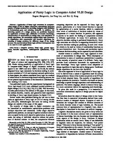
3.8The Resulting PC Architecture A result shown in [6] is that the isolation results cannot be obtained by augmenting the original state set S of the controller with a state that materializes when a VOA occurs. That means the detection must be accomplished by an independent unit. That leads to a architecture with a supervisory level, referred to as the ontological control level, that reads the control action ui,j executed at time t-1 (or t-n for inner state transitions), and the resulting plant formula yk at time t. This information along with state set S is sufficient to determine the de-synchronizations and state transitions. The architecture shown in Figure 3 is based upon the assumption that the state set of the PC is well determined.
3.9Example for an Ontological De-synchronization An example is given below to illustrate the problem of ontological de-synchronization. A position controller has the goal to move a radar antenna into a desired position p. The controller has two inputs: (1) angle φ of the radar antenna given by a mechanical sensor and (2) angle θ of the radar antenna given by an electronic sensor. The measurement of θ is much more accurate than that of φ, however, range ε2 of θ is much smaller than range ε1 of φ. Therefore, the
31
positioning algorithm has two steps: first regulator R1 will bring the radar into the ε2 range of the electronic sensor, then regulator R2 will bring the radar into the desired position p. The position error is ε=q-p, where q can be either φ or θ, depending on the current range. State S1 can be defined as S1=(y1=|εε1 is still satisfied, so the controller will jump again to S7 and the cycle will repeat as predicted by the theory. In order to recover from this situation, a state should be found that corresponds to the current plant situation and which has a control action that can break the cycle. For fuzzy controllers, there can be found recovery solutions by adding extra rules to the rule base [18]. However, for controllers such as PCs that have discrete states, the problem of recovery becomes more difficult since there is no state with acceptable properties in the state space of the controller that can materialize at a VOA. The recovery algorithm proposed in this paper relies on techniques that can accommodate fuzzy states and yet produce crisp outputs for decision making. 4.FSFO-FSM MODEL 4.1Formal Definition The general model of the FSFO-FSM is illustrated in Figure 5, and is given by the formulas:
Z = X o R( y F ) z c = DF ( Z )
(1)
YF = f yF ( X , y F )
where X and Z stand for a finite set of fuzzy inputs and outputs, respectively. R ( y F ) represents the linguistic model of a plant which is now function of the y F present states of the fuzzy state variables and ° is the operator of composition. The zc crisp values of the fuzzy outputs are obtained by computing a DF defuzzification algorithm. Mapping f yF is used to devise the YF
33
next states of the fuzzy state variables from the X fuzzy inputs and the y F present states. Discrete membership functions are assumed. As an initial step to develop the general model of the FSFO-FSM, the concept of the Crisp-StateFuzzy-Output Finite State Machine (CSFO-FSM) model based on two-valued logic was presented in [2]. In the case of the CSFO-FSM, the state set consists of a number of disjoint (crisp) states, and the FSM stays in just one state at a time. The CSFO-FSM model along with State Membership Functions [3] is used to realize the FSFO-FSM model.
An overall linguistic model Rs [3], or a set of linguistic sub-models in the case of multiple-input single-output (MISO) and multiple-input multiple-output (MIMO) systems, repectively, is assigned to each state of the CSFO-FSM. A fuzzy state is defined by a crisp state along with a state membership function:
SFk : Sk , g Sk
where
(2)
S Fk stands for fuzzy state k, Sk represents crisp state k, and g S k is the state membership
function associated with
Sk .
Hence, the FSFO-FSM is represented by the formulas:
34
Z = X o R* R * = G( RS ) z c = DF( Z )
(3)
X B = B( X ) Y = f y ( X B , y)
where R* stands for the composite linguistic model (5), G stands for a matrix of state membership functions (4), XB , Y, and y are two-valued Boolean input and state variables, respectively. B stands for a Fuzzy-to-Boolean transformation algorithm to map a change in the state of a linguistic variable into state changes of a finite set of two-valued variables.
The degree of state membership function is a discrete valued domain set which is typically chosen such that its elements are the same as that of the degrees of membership functions for fuzzy inputs and outputs. A state membership function takes a 1 (full membership) value in just one state of the state set. Let βik denote the degree of state membership to state
S k when the CSFO-FSM is in state
Membership function g Si has a maximum in state Si, hence,
βii
is a maximum (full membership). A graphic interpretation of the state membership function
g Sk is shown in Figure 7. The model of FSFO FSM implemented by CSFO-FSM is shown in Figure 6.
The G matrix of degrees of state membership functions is given by (4).
35
⎡ β 11 ⎢ 2 β1 G=⎢ ⎢ M ⎢ p ⎢⎣β 1
β 12 L β 1p ⎤ ⎥ β 22 L β 2p ⎥ or M
β 2p
L M ⎥ ⎥ L β pp ⎦⎥
⎡ g S1 ⎤ ⎢g ⎥ ⎢ S2 ⎥ ⎢ M ⎥ ⎢g ⎥ ⎢⎣ S p ⎥⎦
(4)
For each fuzzy state of the FSFO-FSM model, a Ri∗ composite linguistic model is created from the finite set of RS i overall linguistic models (i=1,..,p). Let the FSFO-FSM be in fuzzy state S Fk , then
Rk* = max[min(β1k , RS1 ), min(β 2k , RS2 ),..., ..., min(β kk , RSk ),..., min(β kp , RSp )] where
β1k , β 2k ,..., β kp
stand
for
the
degrees
of
state
(5)
membership
function
g S k , and RS1 , RS 2 ,..., RS p are the overall rules in crisp states S1 , S2 ,..., S p , respectively.
With (5), a single-input single-output (SISO) system is assumed. In the case of multiple-input single-output (MISO) and multiple-input multiple-output (MIMO) systems, a set of Rk* composite linguistic models is created analogously with (5), since then each crisp state is represented by a set of overall sub-models [3]. In adaptive systems Rk* is not stored in memory, it is dynamically created by computing (5), instead. By modifying the β degrees of the state membership functions on-line, new R* composite linguistic models can be created under real-time conditions. The switch-over between active R* models is determined by the state transients of the FSFO-FSM. The formulas for linguistic model building and inference computations were given in [3].
36
4.1.1
The B Algorithm
There are two forms of the Fuzzy-to-Boolean Transformation Algorithm, one for fuzzy inputs, and another for fuzzy outputs. Inputs are restricted to fuzzy numbers. Let xc be the average position of the maxima for fuzzy input X that is obtained by applying the Mean of Maxima (MOM) defuzzification algorithm, let k be the number of overlapping linguistic sub-intervals of the universe of discourse (the number of states of a linguistic variable), and let n be the number of non-overlapping, disjoint Boolean sub-intervals. Assuming that the linguistic overlapping factor is 2, then n = 2 k − 1 (for the configuration shown in Figure 8, k=7, n=13). Let X Bi denote the two-valued Boolean input variable which is assigned to disjoint sub-interval i.
X Bi = 1, iff the position of xc falls into Boolean sub-interval i
(i=1,...,n)
and
X Bj = 0 for all j ≠ i ( j = 1,..., n ) . Border points belong to the sub-intervals of lower indices. The leftmost and rightmost positions belong to sub-intervals 1 and n, respectively.
A graphical illustration of the B Algorithm for fuzzy inputs X (1) and X ( 2 ) over a normalized universe of discourse U is given in Figure 8. The same set of linguistic subintervals is assumed for both inputs. Superscripts are omitted for the sake of clarity. Let zc be crisp value of fuzzy output Z (obtained by computing the MOM defuzzification strategy), let λ z denote the height of the maxima and Boolean sub-interval i.
αi
denote the threshold value assigned to
The discrete-valued domain set of α is the same as that of the
membership functions for fuzzy inputs and outputs, respectively.
Let k be the number of
overlapping linguistic sub-intervals of the universe of discourse, and let n be the number of disjoint Boolean sub-intervals (n=2k-1, if the overlap factor is 2). Let Z B i denote the two-valued Boolean output variable which is assigned to disjoint sub-interval I.
37
Z Bi = 1 , iff the zc position falls into Boolean sub-interval i (i=1,...,n) and λ z ≥ α i otherwise
Z Bi = 0.
Z Bj = 0 for all j ≠ i ( j = 1,..., n ) .
A fuzzy output variable is mapped into a finite set of Boolean output variables. In case of MIMO systems, multiple sets of Boolean output variables are created. The state transients of CSFO and FSFO-FSM models, respectively, can be specified in terms of a sequence of changes at the X B Boolean inputs and Z B Boolean outputs. With Boolean outputs, the index of the overall linguistic model by which the fuzzy output is inferred should also be given (e.g.,
).
The two forms of the B algorithm are essentially the same, the one for fuzzy inputs is a special case of the other one for fuzzy outputs, when α i = 0, (i = 1,..., n ) . Using threshold values to evaluate the Z B Boolean outputs allows the tuning of the state transients of the CSFO and FSFO-FSM models.
4.1.2
Specification of the State Transitions
In the further discussion, a SISO model is assumed. The state transitions between dominant states of the FSFO-FSM are specified by means of a sequence of changes in the states of the fuzzy inputs and outputs, respectively. The use of the fuzzy outputs for specifying state transitions is optional. For the sake of clarity, it is assumed the set of states for each fuzzy variable that is used for specifying state transitions of the FSFO-FSM is the same as the one used for model building and inference. First, the mapping of fuzzy states to non-overlapping Boolean sub-intervals for the B algorithm is to be specified. After power up, the FSFO-FSM stays in an initial fuzzy state, say, in S1 with R1* in force. By using the ASM method [23], one can give a condition in terms of the
38
state of fuzzy input X, e.g., being Small, along with the state of inferred fuzzy output Z being Medium to move to fuzzy state S4 in which R4* is in force. The FSFO-FSM stays in state S1, otherwise. By omitting the details of the Fuzzy-to-Boolean transformation, a series of changes in the state of the Boolean variables that result in state transitions can be illustrated as follows: XB3, XB5, XB8, (XB2, ZB7, R4*), XB7, (XB11, R2*), and so on. By specifying Rk* (k = 1,…,p) a state transition from the present state to state Sk will take place. Actually, ZB7 will be considered as an auxiliary input condition. This kind of description can be used to create a source file for a PLD Design language (e.g., XABEL [21]) to design the underlying Boolean finite state machine of the FSFO-FSM. Alternatively, the direct ASM entry format of a professional CAD tool (e.g., Foundation Series by Xilinx Corp. [22]) can be chosen. In either way, the Boolean FSM will be automatically synthesized using contemporary Programmable Logic Devices (FPGAs or CPLDs). In the case of an adaptive fuzzy logic controller based upon the FSFO-FSM model, all α and β values are stored in R/W memory blocks. In addition to tuning the knowledge base, the α and β values can be recomputed and be downloaded into the FLC hardware accelerator.
4.2Outline of the Proposed Recovery Method For the sake of clarity, the use of the FSFO-FSM will be outlined for a single state transition at a VOA. At design time, each plant formula is associated with linguistic intervals. When the state sequence being executed by the PC has arrived at a critical juncture, that is, the next expected state has a set of collateral states associated with it, hence, a VOA might occur. At this point, in order to evaluate the status of the system, and to make a proper decision regarding to the next state of the PC, the Ontological Controller will be downloading the following information to the FSFO-FSM: (i) the fuzzified plant formulas of yi (the last state materialized as expected), of yj
39
(the state with the potential for a VOA), and of the states in K_(Sj), (ii) the overall linguistic models associated with the fuzzy states corresponding to the expected next state, and of the collateral states of the expected next state, (iii) the state membership function degrees for each fuzzy state which are set such that the dominant state is assigned the degree of 1, (iv) the actual mapping scheme between linguistic and Boolean subintervals of the B algorithm. Information (i) will be considered as fuzzy input vector X to the FSFO-FSM, (ii) and (iii) will be used to create the R* composite linguistic model in the next fuzzy state, and (iv) will be used to make a transition to the next fuzzy state. If a VOA has occurred, a fuzzified plant formula in-between the expected next state yj and one of its collateral states will be passed to the FSFO-FSM. There are two main approaches to tackle the problem of recovery from a VOA by using the FSFO FSM. One of them is to deal with it as a condition for state transition to the next fuzzy state. The conditions for state transitions are given in terms of fuzzified plant formulas (i.e., membership functions). If the received actual, fuzzified plant formula is not too far from the one that is specified to make a transient to state yj, then the FSFO-FSM will enter to a fuzzy state that corresponds to yj. The control action inferred from the Rj* composite linguistic model will cause the system to recover from the VOA. Otherwise, the FSFO-FSM will move to one of the states in K_(Sj). That means the PC cannot recover from the VOA, hence, it should be halted. If no VOA has occurred, the FSFO-FSM will move to the expected next state. After a fuzzy state transition has taken place, the FSFO-FSM will pass the inferred (defuzzified) output(s) back to the Ontological Controller that will make the decision on setting the goal path for the PC. In the case of the other approach, the FSFO-FSM will enter a fuzzy state that does not correspond directly to neither yj, nor any state in K_(Sj). The β degree of state membership for yj has a value of less than 1 in that state. On the basis of the information returned by the FSFO- FSM, the
40
Ontological Controller has detected the ontological de-synchronization, and it will attempt to dynamically tune the β degrees of state membership functions using fuzzy set theory methods in order to recover from the VOA. That is, a suitable R* model is to be found such that the inferred control actions will allow the system to break out of the cycle and proceed along a proper goal path. During design time, the intervals used for the plant formulas of the state sets are set, in fact, as crisp, disjoint ones. However, fuzzification makes the boundaries between crisp states of the PC continuous such that a state preserves its properties beyond its Boolean limits. Thus fuzzification balances the fuzzy boundaries of the states against the degree of the ontological violation. It allows to find a control action (if any) to recover from the VOA.
5.SIMULATION OF THE RECOVERY PRINCIPLE A program using C++ has been developed to simulate various fuzzy finite state machine models. This program has been designed to model a HFB-FSM [24] that is an extension of the FSFOFSM architecture. The basic information which the user should provide for the HFB-FSM simulator includes: the number of fuzzy inputs and outputs, the number of Boolean inputs and outputs, the number of fuzzy and crisp states, state membership functions, fuzzy input and output universal sets along with the associated Boolean sub-intervals for the B algorithm, conditions for state transitions, and lastly, the rule sets that model the system’s performance in each crisp state. In the case of the FSFO-FSM, some of these features are not used. The program provides for a choice of six different implication functions. In each crisp state an aggregated rule base is constructed according to the mathematical models of SISO, MISO and MIMO systems [25]. The user can tune the adjustable parameters of the system (e.g., state membership degrees, Boolean
41
sub-intervals and threshold values of the B algorithm) in order to get the desired results. The inferred fuzzy outputs are processed by a defuzzification algorithm selected by the user from a list. Out of the two approaches outlined in Section 4.2, the one that deals with the problem of recovery as a state transition of the FSFO-FSM will be presented in the sequel. It is assumed in this paper that the OC needs just crisp information on the status of the system, e.g., a VOA has occurred but the system can recover from it. Quantifying the strength of the recovery will not be a requirement. Yet to sort out normal system operation from a VOA, the FSFO-FSM should also furnish the OC with the information whether the two measurements are sufficiently aligned, or they are not. A simple way to accomplish that is to reduce the FSFO-FSM to a CSFO-FSM, and to split both states S3 and S7 into two crisp states each. In each of the four crisp states, the linguistic model can be set up such that only one fuzzy output will be inferred in the form of a fuzzy singleton. Hence, no actual defuzzification will be needed. The block diagram used for the simulation of the position controller is shown in Figure 9. For the sake of clarity, only data relevant for this example will be discussed. In Figure 9, φ and θ stand for the angle measurement from the mechanical and the electronic sensor, respectively, φF and θF represent the measurements in fuzzified form, and ZF stands for the fuzzy output provided by the FSFO-FSM for the Ontological Controller (OC). When the state sequence executed by the PC has progressed to state S2 (Figure 4), the OC will send the fuzzified measurement (φF and θF) along with the index of the current fuzzy state (SF2) to the FSFO FSM. In fact, for this example, it will be crisp state S2. Then the FSFO-FSM, on the basis of the fuzzy input data, will make a transition to the next state, and in turn, will also determine whether the two measurements are
42
sufficiently aligned, or they are not. This information will be returned to the OC and the appropriate action will then be taken. To conduct a simulation of the recovery, two fuzzy variables are introduced as follows: the difference of the angle position by the mechanical sensor and the desired angle position (eφ = ⏐φ p⏐), and the difference of the angle by the electronic sensor and the desired angle (eθ = ⏐θ - p⏐). Three linguistic labels have been chosen for each variable as follows:
UR: Under Range, IR:
In-Range, and OR: Over Range, with respect to the work range of the sensors, and regulators R1 and R2, respectively The associated membership functions for these linguistic labels are illustrated in Figure 10. The plant formulas for states S2 and S3 are given such that S2: ⏐φ - p⏐< 16, and S3: ⏐θ - p⏐< 10. For the B algorithm, the universal set of each fuzzy input is mapped to five disjoint sub-intervals as follows: XB1 = [0 , 6) XB2 = [6 , 10) XB3 = [10 , 13) XB4 = [13 , 16) XB5 = [16 , 38) These sub-intervals are used for the B algorithm in order to determine the next state of the FSFOFSM. The state transition graph for the crisp (dominant) states is shown in Figure 11. The OC will evaluate the fuzzy singleton outputs as follows: ZF0 - next state is S3, a VOA has occurred (the two measurements are not aligned) but the system can recover, ZF1 – next state is S3, the status of the system is normal (the two measurements are aligned), ZF2 - next state is S7, a VOA has occurred (the two measurements are not aligned), recovery is not possible, ZF3 - next state is S7, a VOA has occurred (however, the two measurements are aligned). The fourth output can be viewed as a “don’t care” condition in terms of digital system design, that is, it cannot occur. The
43
notation (i-j) refers to the condition that the defuzzified φF and θF values fall into disjoint subintervals ‘i’ and ‘j’, respectively. The simulation results for five different scenarios are illustrated in Figure 12. In the first case, illustrated in Figure 12(a), both measured angles fall into XB4. It means that even after considering uncertainty in measurement, plant formula for S3 is not materialized, hence, the system cannot recover from the VOA. The next state of the FSFO-FSM will be SF7-A. However, the two measurements are sufficiently aligned thus the output returned is ZF3. In Figure 12(b), since the angle value by the electronic sensor falls into XB3, the plant formula for S3 is materialized, hence, the system will recover from the VOA. The FSFO-FSM will move to state SF3-R. The two measurements are not aligned thus the output returned is ZF0. Figure 12 (c) exhibits a big offset between the two measurements. However, the electronic sensor
in this range in considered more accurate than the mechanical one. It is then decided the antenna is not yet in the range for regulator R2, so the next state of the FSFO-FSM will be SF7-NA. It is obvious that the measurements are not aligned, the output will be returned as ZF2. In Figure 12(d) and (e), both measured angles fall into subintervals XB2, or XB3 that is the desired condition for the plant formula in state S3. Figure 12(d) illustrates a recovery from a VOA, while a normal transition to state S3 is shown in Figure 12(e).
6.CONCLUDING REMARKS The use of the FSFO-FSM model proposed in this paper represents a departure from the traditional application of fuzzy logic in controls. Traditionally, the advantage of using fuzzy logic has been associated with properties such as faster execution of the control algorithm, lower memory requirement, and more intuitive representation of the plant. These properties have been
44
favorably compared to performance measures of more traditional methods. In ontological control, the FSFO-FSM approach represents a recovery method for sequential controllers. This method, until now, has no known alternatives. The existence of such a method opens a way to design robust autonomous systems such as unmanned vehicles, complex control systems, and alike that can detect and recover from unexpected changes in their environment. Further research will be done to extend the FSFO-FSM model in order to treat both fuzzy and two-valued inputs and outputs, respectively, within the same architecture. Another research goal is to quantify the strength of the recovery.
7.
ACKNOWLEDGEMENTS
This research was supported by the Michigan Space Grant Consortium (Grant #: 9633401), Western Michigan University, ABB Automation Products AB, Sweden, and The Swedish Research Council for Engineering Sciences (271/96-134).
7.8.
REFERENCES
[1]
D. Driankov, G. Fodor, Ontological Real-Time Control, Proc. and Plenary Talk, First
European Congress on Fuzzy and Intelligent Technologies, Aachen, Germany, Sept. 1993. [2]
J. Grantner, M. Patyra, M. Stachowicz, Intelligent fuzzy controller for event-driven real time systems and its VLSI implementation, in the book Fuzzy Control Systems (Eds. A. Kandel, G. Langholz), pp. 161-179, CRC Press, Boca Raton, FL, USA, 1994.
[3]
J. Grantner, M. Patyra, VLSI implementation of fuzzy logic finite state machines, IFSA ´93 World Congress, Proceedings Vol. II, pp. 781-784, Seoul, Korea, July 4-9, 1993.
45
[4]
Ramadge, P.J.G., Wonham, W. M. The Control of Discrete Event Systems. In Proc. of the IEEE, vol. 77, no. 1, Jan. 1989, pp. 81- 97.
[5]
Eriksen, T.J., Heilmann, S., Holdgaard, M., Ravn A.P. Hybrid Systems: A Real-Time Interface to Control Engineering, Proc. of the 8-th Euromicro Workshop on Real-Time Systems, 1996.
[6]
G. Fodor, Ontologically Controlled Autonomous Systems: Principles, Operations and Architecture, Kluwer Academic Publishers, Boston / Dordrecht / London (1998).
[7]
J. Grantner, Design of event-driven real-time linguistic models based on fuzzy logic finite state machines for high-speed intelligent fuzzy logic controllers, Thesis for the Degree Candidate of Technical Science, Hungarian Academy of Sciences, Hungary (1994).
[8]
A. Sanchez, Formal Specification and Synthesis of Procedural Controllers for Process Systems. Lecture Notes in Control and Information Sciences 212, Springer-Verlag London Limited 1996.
[9]
Benveniste, A., Åström, K. J., Caines, P.E., Cohen, G., Ljung, L., Varaiya, P., Facing the challenge of computer science in the industrial application of control: a joint IEEE CSSIFAC project, in IEEE Transactions on Automatic Control, vol. 38, No.7 July 1993.
[10]
International Electrotechnical Commission, International Standard, Programmable Controllers Part 3: Programming Languages, IEC 1131-3.
[11]
Hatley, J.D., Pirbhai, I.A., Strategies for Real-Time System Specification, Dorst House Publishing, New York, 1987.
[12]
Lin, Jing-Yue, Ionescu, Dan., A generalized temporal logic approach for control problems of a class of non-deterministic discrete event systems, Proc. of the 29-th IEEE Conf., Decision and Control, Honolulu, Hawai, Dec. 5-7, 1990, pp. 3440-3445.
46
[13]
Feng Lin, Analysis and Synthesis of Discrete Event Systems Using Temporal Logic, in the Proceedings of the 1991 IEEE International Symposium on Intelligent Control, 13-15 August 1991, Arlington Virginia, USA.
[14]
Antsaklis, P. et al., Report of the Task Force on Intelligent Control, IEEE Control Systems Society, Dec. 1993.
[15]
René David, Grafcet: A Powerful Tool for Specification of Logic Controllers, in the IEEE Trans. on Control Systems Technology, vol. 3, no. 3, Sept. 1995, pp. 253-268.
[16]
J. Grantner, M. Patyra, Synthesis and analysis of fuzzy logic finite state machine models, WCCI’94, Proceedings the FUZZ-IEEE’94, Vol. I, pp. 205-210, Orlando, FL, June 2629, 1994.
[17]
G. Fodor, Ontological Control: Description, Identification and Recovery from Problematic Control Situations, Ph.D. Thesis, Dept. of Computer Science, University of Linkoeping, Sweden, 1995.
[18]
D. Driankov, G. Fodor, Fuzzy control under violations of ontological assumptions, Invited plenary talk, FLAMOC'96 Proceedings, pp. 109-115, Sydney, Australia, Jan. 1518, 1996.
[19]
G. Fodor, J. L. Grantner, D. Driankov, Modeling the real-time recovery of complex control systems- a fuzzy approach, Proceedings of the IEEE-SMC’97 Conference, Vol. 3, pp. 2163-2168 (Oct. 1997)
[20]
P.J. Antsaklis, K.M. Passino, An Introduction to Intelligent and Autonomous Control, Kluwer Academic Publishers, Boston/Dordrecht/London, 1994.
[21]
Xilinx – ABEL Software Design Reference Manual, 981-0300-002, November 1993.
[22]
Foundation V. 1.5, Xilinx Corp., 1998
47
[23]
C. R. Clare, Designing Logic Systems Using State Machines, McGraw-Hill Book Co., 1973.
[24]
J.L. Grantner, G. Fodor, D. Driankov, Hybrid Fuzzy-Boolean Automata for Ontological Controllers, Proc. of the 1998 World Congress on Computational Intelligence, FUZZIEEE’98/WCCI’98, vol. I, pp. 400-404, Anchorage, Alaska, May 4-9, 1998.
[25]
Janos L. Grantner, Parallel Algorithm for Fuzzy Logic Controller, in the book Fuzzy Logic: Implementation and Applications (Eds.: M. J. Patyra, D. M. Mlynek), John Wiley and Sons, and B. G. Teubner Publishers, 1996, ISBN Wiley: 0 471 95059 9, pp. 177-195.
[26]
Shaoying Liu, A. Jeff Offutt, Chris Ho-Stuart, Yong Sun, Mitsuru Ohba. SOFL: A Formal Engineering Methodology for Industrial Applications, IEEE Transactions on Software Engineering, Vol. 24, No.1, January 1998.
8.FIGURES AND TABLES Table 1 De-synchronization type VOA Unexpected external actions Timing Ill-represented formula
De-synchronized state transition p q Si → Sj p q Si → Sj p q Si → Sj p q Si → Sj
Materialized state after de-synchronization q in K-(Sj ) p in K-(Si ) q in K-(Sj ) not in S
48
p
q
Si
Sj
p,q ui,j
p
(zi, c i )
q j
(zj , c )
ext
u i,k
s
p
Sk
Sn
p,s
u k,n
p
(zk ,c k )
s
(zn ,c n)
Figure 1. State transition due to external action
Si
q
p
(ci ,z
r
Sj p ) i
u
Sk
p,q i,j
q,r
(c j ,z
u j,k
q )j
r
(c k,z k)
u ext j,l t Sl
s Sn
t,v
s,t
(c n,z
s ) n
u n,l
v
Sm
(c l ,z
t ) l
u l,m
Figure 2. Non specific control configuration
v
(cm,z m)
49
external actions
Plant plant output
control actions u i,j
y
k
Programmable Controller S=(yi , ui,j )
Delay
u voa-oc Ontological Controller S
ui,j (t-n)
oc yk (t)
Figure 3. Architecture with Ontological Controller
S0
S tart R 1
S1
R1
S2
A cting
S
R2 A cting
S top R 1 3 S tart R 2
S4
G oal A ction
VOA
disturbance disturbance
S6
S7
Figure 4. The state set of a position controller
S5
50
X
.. .
Z = X o R (y F z c = D F (Z )
. y .. F
. . . ..
)
Y = fy (X ,y ) F F F
. . .
Z zc
YF
F u zzy M em o ry E lem en ts
Figure 5. General model of the FSFO-FSM
Z = X o R* R * = G (Rs ) z c = D F (Z )
X SM F M e m o ry
yF y
X B = B (X ) Y = yf (XB ,y )
Z zc
Y
M e m o ry E le m e n ts
Figure 6. Model of the FSFO-FSM implemented by the CSFO-FSM
51
gs
k
❂ k ❂k - 1
1 0 .8 0 .5 0 .3 0
k k
k ❂k + 1
S 1
2
k - 1
k
k +p 1
Figure 7. Graphic interpretation of state membership function g Sk
X
(1)
or X
(2)
1
U 0 X B1
XB2
X B3
X B4
X
B5
X
B6
X B7
X B8
X B9
X B10 X
B11
X B12
X B13
Figure 8. Fuzzy and Boolean subintervals for fuzzy inputs
52
φ θ
Action
PC
Current State
Next State
OC
φF θF
ZF
FSFO-FSM
Figure 9. OC configuration with the FSFO-FSM
IRφ
URφ
ORφ
1
0
6
URθ
10
30
IRθ
34
38
eφ
38
eθ
ORθ
1
0
4
10
16
Figure 10. Fuzzified membership functions for eϕ and eθ
53
ZF0 SF3-R
(4-3), (4-2), (3-2), (2-3)
SF2
(2-2), (3-3)
ZF1 SF7-N (2-4), (3-4) 1 (4-4)
ZF2
ZF0 ZF1 ZF2 ZF3
SF7-NA
ZF3 SF7-A Figure 11. Fuzzy state transition graph
ZF
54
θF
1
(a)
0
10
0
10
(d)
0
φF
0
6 8
0
12
14
12
1
Next state: SF3-R , ZF0
16
Next state: SF7-NA , ZF2
16
θF
Next state: SF3-R , ZF0
12
φF
8
16
θF
6
1
(e)
14
Next state: SF7-A , ZF3
φF
φF
1
(c)
12
θF
1
(b)
φF
16
θF
10
12 14
Next state: SF3-N , ZF1
16
Figure 12. Simulation results
55
NOMENCLATURE VOA - violation of the ontological assumptions FSFO-FSM – Fuzzy-state fuzzy-output finite state machine plant PC - programmable controller WDSS - well-determined PLD – Programmable Logic Device ASM – Algorithmic State Machine FPGA – Field Programmable Gate Array CPLD – Complex PLD FLC – Fuzzy Logic Controller R/W – Read/Write HFB-FSM – Hybrid Fuzzy-Boolean Finite State Machine