Applications of a semi-dynamic convex hull algorithm - Semantic Scholar

BIT 32 (1992), 249-267.

APPLICATIONS CONVEX

OF A SEMI-DYNAMIC HULL

ALGORITHM

JOHN HERSHBERGER and SUBHASH SURI DEC Systems Research Center, 130 Lytton Avenue, Palo Alto, CA 94301, USA

Bell Communications Research, 445 South Street, Morristown, NJ 07960, USA

Abstract. We obtain new results for manipulating and searching semi-dynamic planar convex hulls (subject to deletions only),and apply them to derive improved bounds for two problems in geometry and scheduling. The new convex hull results are logarithmic time bounds for set splitting and for finding a tangent when the two convex hulls are not linearly separated. Using these results, we solve the followingtwo problems optimally in O(nlogn) time: (1) [matching] given n red points and n blue points in the plane, find a matching of red and blue points (by line segments) in which no two edges cross, and (2) [scheduling] given n jobs with due dates, linear penalties for late completion, and a single machine on which to process them, find a schedule of jobs that minimizes the maximum penalty. CR categories: F.2.2, 1.3.5, E..1. Additional keywords: Convex hull, semi-dynamic algorithm, geometric matching, scheduling.

1. Introduction. The convex hull is a versatile and well-studied structure in c o m p u t a t i o n a l geometry. It has n u m e r o u s applications, including statistical trimming, range searching, and facility-location problems in operational research. N o t surprisingly, computing the convex hull is one of the best-investigated problems in c o m p u t a t i o n a l geometry, In two dimensions, an O(n log n) time algorithm for c o m p u t i n g the convex hull of n points has been k n o w n since 1972 [9] - several other algorithms have been discovered since then; see Preparata and S h a m o s [18] or Edelsbrunner [6] for a survey. A tight b o u n d on the problem was ultimately achieved by Kirkpatrick and Seidel [13], w h o showed that O(n log h) is both an upper and lower b o u n d for the planar convex hull problem, where h denotes the n u m b e r of points on the hull. In m a n y applications, one needs dynamic convex hulls, where points can be inserted or deleted from the set. The best b o u n d currently k n o w n for the dynamic convex hull problem is due to O v e r m a r s and van Leeuwen [16], w h o show that Received January 1991. RevisedOctober 1991.

250

JOHN HERSHBERGER AND SUBHASH SURI

a convex hull can be maintained at a worst-case cost of O(log 2 n) per insertion or deletion. Better results are possible, however, if there are only insertions or only deletions. In the case of insertions, an algorithm due to Preparata [17] can insert a new point and update the convex hull in worst-case time O(log n). The case of deletions is a little more complicated, but it is possible to process a sequence of n deletions in O(log n) amortized time per deletion (see Hershberger and Suri [11]; the same result is also implicit, though not pursued, in the convex layers paper of Chazelle [5]). In this paper, we work with a deletions-only convex hull. Starting with a set of n points, our algorithms perform an online sequence of deletions intermixed with searches and manipulations on the current convex hull. Our applications require two key operations: (1) finding a common tangent of two convex hulls that are not necessarily separated by a line, x and (2) the set-splitting operation, in which we split our data structure in two by a vertical line so that the points to the left of the line go into one structure and the points to the right go into the other. We achieve an O(logn) time bound for both these operations; the bound is amortized for the set-splitting operation. (Overmars and van Leeuwen [ 16] also have an O(log n) time algorithm for finding a common tangent, but their method works only for linearlyseparated convex hulls.) Using these results, we obtain improved algorithms for the following two problems: (Matching)given n red points and n blue points in the plane, find a matching of red and blue points by line segments in which no two segments cross, and (Scheduling)given n jobs with due dates, linear penalties for late completion, and a single machine on which to process them, find a schedule of jobs that minimizes the maximum penalty. We achieve O(nlog n) time for both these problems, which is optimal in the worst case. 2 Our data structure and the accompanying analysis can be applied to achieve an O(log n) time bound per operation for some special cases of intermixed insertions and deletions. These extensions, interesting in their own right, may also be useful for attacking the general problem of maintaining fully dynamic convex hulls. This paper is organized in six sections. In Section 2, we describe our basic data structure for maintaining and searching a deletions-only convex hull. Sections 3 and 4 show how to strengthen this data structure to allow two additional operations: finding common tangents of two deletions-only hulls, and splitting the point-set at a given x-coordinate. Applications are discussed in Section 5. We conclude in Section 6 with some extensions and open problems.

1 A c o m m o n tangent of two convex hulls is a line that touches both hulls but does not intersect the interior of either. 2 A third application, included in the conference version of this paper (SWAT '90, pp. 380-392), is an algorithm for covering a set of n points by two disks of specified radii. Because that algorithm improves a result from the conference version of our paper on tailored partitions (ACM Symp. on CG, 1989, pp. 255-265), we have chosen to omit it from this paper and include it in the journal version of the tailored partitions paper [11].

APPLICATIONS OF A SEMI-DYNAMIC CONVEX HULL ALGORITHM

251

2. The basic data structure.

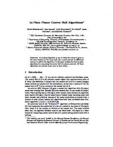
In this section we describe our basic data structure for maintaining and searching the convex hull of a planar set of points during an online sequence of deletions. We are given a fixed set of points S that underlies all the updates, with ISl = n. Starting with a subset P _~ S, we would like to maintain the convex hull of P as points are deleted online from P. For convenience, we split the sequence of convex hull edges at its leftmost and rightmost vertices to obtain an upper hull and a lower hull. We consider only the problem of maintaining the upper hull of P, denoted h(P). Our underlying data structure is a complete binary tree whose leaves correspond to the points of S in x-order; the same basic structure is also used by Chazelle [5] and Overmars and van Leeuwen [ 16]. The tree is the interval tree for S [ 18]; we denote it by 1(S). With every node v ~ I(S), we associate a set S(v) and an x-coordinate x(v): the set S(v) is the subset of S corresponding to the leaves below v, and x(v) is the midpoint of the interval bounded by the rightmost point of S(leftson(v)) and the leftmost point of S(rightson(v)). (If v is a leaf, then x(v) is simply the x-coordinate of the corresponding point.) We represent a subset P ~_ S by an upper portion of the tree I(S), denoted by T(P). This subtree T(P) changes as points are deleted from P, but the interval tree I(S) remains fixed throughout. Let us define P(v) = P c~ S(v). The nodes of T(P) are the leaves of I(S) that contain points of P, along with their ancestors; that is, a node v ~ 1(S) is copied into T(P) if and only if P(v) is nonempty. Refer to Figure 1 for an example. We endow this basic subgraph with additional node-fields to represent the upper hull h(P). We call the full data structure a hull tree. A hull tree node v represents h(P(v)), the upper hull of the points from the leaves below v in T(P). Storing the entire hull h(P(v)) at each node v would be convenient for searching and manipulating h(P), but would unfortunately require a superlinear amount of storage. In order to reduce the space complexity to linear, we store only a portion of h(P(v)) at the node v. To explain what points are stored where, we need the notion of the level of a point, which is also crucial for our amortization arguments. Consider a point p ~ P, and let u be the corresponding leaf of T(P). Now, p is obviously a vertex of the convex hull h(P(u)); it may also belong to hulls represented by ancestors of u. Let v be the highest ancestor of u for which p is a vertex of h(P(v)); node v may be the root of T(P). We define the level of p, written level(p), to be the depth ofv in T(P). The point p e P is stored at node v e T(P) - that is, at the node that gives p its level. It might appear that this storage scheme fragments the hulls rather arbitrarily. However, this is not the case: because the line x = x(v) separates the points associated with the left and right children of v, hull partitioning has a particularly simple form. To illustrate, let I and r denote the left and right children ofv. We determine the hull h(P(v)) by finding the common tangent of h(P(l)) and h(P(r)). Then the portions of h(P(1)) and h(P(r)) hidden by the common tangent are precisely the fragments stored at I and r. The root of T(P) stores the current hull h(P) in its entirety.

252

JOHN HERSHBERGER AND SUBHASH SURI

/

A

2

",X, ,'11 p ffi [] Fig. 1.

/

~

\

F

,'1/ .,'Ak ~

T(P)

\

A

P(v)

T(P) is a subgraph of I(S).

Node v of the hull tree data structure has two fields. The first is a pointer to a doubly-linked list of points, denoted by chain(v), which represents h(P(v)) or the hidden fragment of it mentioned above. The second field, denoted by tan(v), represents the common tangent of h(P(l)) and h(P(r)) by pointers to its endpoints in chain(v). If chain(v) represents h(P(v)), and chain(1) and chain(r) represent the hidden fragments of h(P(l)) and h(P(r)) produced while constructing h(P(v)), then we can use tan(v) to reconstruct h(P(1)) and h(P(r)) from these components in constant time. As T(P) is built, the endpoints of tan(v) may be spliced out of chain(v) and moved to chain(w) for some other node w. However, the pointers in tan(v) are not invalidated by this splicing, and whenever chain(v) is restored to represent h(P(v)), we can use tan(v) to form h(P(1)) and h(P(r)) from h(P(v)) in constant time. With this high-level description of our data structure at hand, we now state several technical lemmas, which together establish our main result in this section (Theorem 2.6). LEMMA2.1. Let P ~_ S be a given set of points on which we perform a sequence of deletions. Then level(p) is nonincreasing during the lifespan of any point p ~ P. PROOF. When a point d is deleted from P, every vertex of h(P) except d remains a vertex of h(P\{d}). This also holds for h(P(v)) for every node v E T(P), which proves the lemma. • This lemma forms a critical part of the analysis of our data structure. The lemma says that when we delete a point from P, other points of P can move only upward in T(P). Since the height of T(P) is ['log2 n], the total number of point-level movements (percolations) is O(n log n). To process each deletion, our algorithm uses the follow-

APPLICATIONS OF A SEMI-DYNAMIC CONVEX HULL ALGORITHM

253

ing lemma, which allows us to perform a deletion in time O(log n + k), where k is the total number of percolations caused by the deletion. We use the notation a . . . b to refer to a convex chain with endpoints a and b. LEMMA2.2. Suppose that L and R are two upper hulls lying to the left and right, respectively, of some vertical line. Let lr be their upper common tangent, with t ~ L and r ~ R. Let p ~ L and q ~ R be two points that lie to the left ofl and r, respectively. Then, given p and q, we can compute I and r in time O(k), where k is the total number of hull vertices in the subchains p . . . I and q . . . r. PROOF. Because Ir is a common tangent of L and R, the two upper hulls have the same slope at I and r. (More precisely, the minimum slope of the edges left of I on L and left of r on R is greater than the maximum slope of the edges right of I and r.) We can find I and r by merging the edge lists of L and R by slope, starting from p and q and stopping when we reach I and r (which we can detect by a purely local test). This'takes constant time per edge examined, or O(k) altogether. • Using the previous two lemmas, we can construct the convex hull of P and then delete points online in 0 (log n) amortized time each. LEMMA2.3. Given a set o f points P ~_ S, IPI = m, we can construct the hull tree T(P) in O(m log n) time. PROOF. The underlying tree of T(P) has O(min(n, IPI log n)) nodes. We build this tree in O(IP) log n) time by copying every node of I(S) for which S(v) n P is nonempty. We fill in the other fields of T(P) by a bottom-up merging process. Initially, we set chain(v) = P(v) for each leaf v. At each merging step, we compute the common tangent of two upper hulls. Suppose we wish to fill in the fields of a node v with children u and w. The chains chain(u) and chain(w) contain the upper hulls of P(u) and P(w). We apply Lemma 2.2 to find the common tangent, taking p and q to be the leftmost vertices of chain(u) and chain(w). We cut the two child chains at the tangent endpoints and link the outer pieces to get the chain for h(P(v)). We store this in chain(v) and leave the inner chain pieces behind in chain(u) and chain(w); the points in those chains have reached their level. We finish by storing pointers to the tangent endpoints in tan(v). The construction takes o(Ie(v)l) time for each node v, or O(IP1) time for each level of T(P). There are flog2 n'] levels, which proves the lemma. • LEMMA2.4. Given T(P), we can delete a point o f P in amortized time O(logn). PROOF. Let d be the point to be deleted from P, and let z be the leaf of T(P) that contains d. We need to update chain(v) and tan(v) for every ancestor v of z. The algorithm to do this is shown below in pseudocode.

254

JOHN HERSHBERGER AND SUBHASH SURI

Procedure Delete (d, v) (* Delete a point d from the subtree of T(P) rooted at v. The left and right children of v are u and w. W L O G assume d e P(w); the other case is symmetric. Let I and r be the endpoints of tan(v). On entry, chain(v) represents h(P(v)). On exit, chain(v) represents h(P(v)\{d}). *) Use tan(v) to restore chain(u) and chain(w), disassembling chain(v). if chain(w) = {d} then (* P(w) = {d} *) Set the right child pointer of v to NIL. Set tan(v) ,,- NIL; chain(v) ~- chain(u); chain(u) ,.- NIL;

else p ~ t; (* now in chain(u) *) if d = r then q ~- left neighbor of d in chain(w); else q *-- r; endif; Call Delete(d, w); (* p and q remain valid after the call *) Use Lemma 2.2 to find the upper common tangent of chain(u) and chain(w). Cut and splice chain(u) and chain(w), creating chain(v) and shortening chain(u) and chain(w). Set tan(v). endif

end Procedure We start the deletion routine by calling Delete(d, root), where root is the root of T(P). Each step of the Delete procedure except the tangent-finding and the recursive call takes only constant time. The number of calls is bounded by the height of T(P), which is O(log n). To bound the tangent-finding time, we relate the points walked over by the algorithm of Le'mma 2.2 to point-level percolations. Ifd ~ r, then tan(v) does not change, and reconfirming it takes O(1) time. If d = r, then the new left endpoint of tan(v) is to the right of the old one, and the right endpoint of tan(v) lies on a subchain ofh(P(w)\{d}) bounded by the old neighbors ofd on h(P(w)). Thus we can apply Lemma 2.2 with p and q as set by the Delete procedure. Let the endpoints of the new tan(v) be l' and r'. On the left side, the vertices of chain(u) between p and l' move from chain(u) up to chain(v). On the right side, the vertices of chain(w) strictly between q and r' were moved from some lower chain up to chain(w) by the deletion of d. Thus the cost of tangent-finding is bounded by the number of percolations at the level ofv and its children. Summed over all the calls needed to delete all the points of P, the total tangent-finding cost is O([Pt log n), or O(log n) per deletion. • Finally, we show that our representation of the convex hull supports the standard repertoire of binary searches. A typical binary search proceeds by performing tests with the tangent edges stored at the nodes of T(P). In an earlier paper 1-11], we

APPLICATIONSOF A SEMI-DYNAMICCONVEXHULL ALGORITHM

255

represented h(P) by a search tree that emulated the hull-chain stored at the root of T(P). The following lemma removes this complication. LEMMA 2.5. Using the tangent edges stored at nodes of T(P), we can perform a binary search on the node-list ofh(P). In particular, the following primitives can be implemented in O(log n) worst-case time: 1. find a tangent to h(P) from a point outside the hull, 2. find an extreme vertex of h(P) in a query direction, 3. find the intersections ofh(P) with a query line, and 4. determine whether or not a point lies inside h(P). In addition, ilL and R are two x-separated subsets of S stored in the hull trees T(L) and T(R), respectively, then we can find the outer common tangents of h(L ) and h(R ) in time O(log n). PROOF. Every edge ofh(P) appears as tan(v) for some node v. The subtree of T(P) rooted at a node v represents h(P(v)) by the tangent edges stored at its nodes. The search algorithms are standard: they look at tan(root), where root is the root of T(P), then recursively search in one of the two subtrees. For example, to find the tangent(s) to h(P) from a point outside it, we look at tan(root), decide whether the point of tangency lies to the left or fight of tan(root) in h(P(root)), and then recursively search in the appropriate tree. A tangent to the selected subchain is also a tangent to h(P). Finding an extreme vertex is the same as finding the tangent through a point at infinity. We determine containment of a point by a recursive search to find an edge of h(P) whose projection on the x-axis contains the projection of the point. We find intersections with a line by searching for the left and right intersections separately, which makes this search fit the given framework. We can find the outer common tangents of h(L) and h(R) in O(log n) time using the algorithm of Overmars and van Leeuwen [16]. [] The main result of this section is summarized in the following theorem. THEOREM 2.6. Let S be a fixed set of points, [St = n, and let P ~_ S be a subset, IPI = m. In O(m log n) preprocessing time, we can build a data structure representing the convex hull of P such that the data structure (1) uses O(min(n, m log n)) space, (2) supports the search queries of Lemma 2.5, and (3) allows online deletion of points from P in O(log n) amortized time per deletion. Our data structure as described so far is quite similar to, although a bit simpler than, the one we used for circular hulls in our paper on tailored partitions [11]. We extend this basic structure to allow more general types of search and manipulation in the next two sections.

256

JOHN HERSHBERGERAND SUBHASHSURI

3. Searching on two convex hulls. Let R (red) and B (blue) be two disjoint sets of points in the plane, where tRI and tBI are O(n). We wish to maintain the (upper) convex hulls of R and B, allowing deletions, such that at any time a common tangent of h(R) and h(B) can be computed in logarithmic time. Recall that Theorem 2.6 allows us to maintain the two hulls, h(R) and h(B), at an amortized cost of O(log n) per deletion. The tangent-finding problem, however, can be tricky: given two arbitrary convex polygons of n vertices each, we need t2(n) time in the worst case to find a common tangent. The lower bound is easily illustrated by the following example: if we have two nested polygons, with the inner polygon protruding one of its vertices slightly across an edge of the outer polygon, an algorithm will be forced to examine all the vertices of both polygons. In general two convex hulls may have a linear number of common tangents between them, but we are content with finding just one. In view of the lower bound mentioned above, we clearly need some additional information about the two hulls to speed up the tangent-finding operation. Overmars and van Leeuwen have shown that if we know a line that is guaranteed to cut the tangent, then the tangent can be found in O(log n) time [16]. Our method also uses this fact, but the difficulty in our case stems from not knowing such a line a priori. (In Overmars and van Leeuwen's case, the existence of such a line is trivially guaranteed, since their two hulls are always separated by a vertical line.) Indeed, most of our effort is spent in determining a line that is guaranteed to cut the tangent. Once such a line is found, we invoke the tangent-finding method of Overmars and van Leeuwen [16]. In what follows, we say that the x-interval of a point set is the interval defined by the minimum and maximum x-coordinates of the points in the set. Our main result in this section is this: given two sets of points R and B, we can maintain their upper convex hulls with deletions so that at any instant if the x-intervals of the two sets do not nest (neither contains the other), then we can find an upper common tangent in logarithmic time. It is crucial for the logarithmic bound that we know R u B in advance; if R and B are not preprocessed together (for example, if the upper hulls of R and B are stored in separate x-ordered arrays without any additional data structures), then f2(log 2 n) time is a lower bound for finding a tangent [10]. Our approach is similar to that used by Guibas, Hershberger, and Snoeyink [ 10]. Rather than finding an upper common tangent of h(R) and h(B) directly, we work on the "dual" problem, which is to find an intersection point of the two hulls. That is, we maintain the upper convex hulls of R and B, so that whenever their x-intervals overlap without nesting, we can find an intersection point of the hulls in logarithmic time. Given an intersection point, we can use Overmars and van Leeuwen's algorithm to find a tangent - a vertical line through the intersection point cuts the tangent edge. In the following discussion, it is convenient to assume that an upper convex hull begins and ends with vertical rays to - oo. We denote these extended

APPLICATIONS OF A SEMI-DYNAMIC CONVEX HULL ALGORITHM

257

hulls also by h(R) and h(B), respectively. Observe that if the x-intervals of R and B overlap but do not nest, then their vertical rays alternate along the x axis. 3 If the x-intervals are disjoint, we can apply Lemma 2.5 to find a tangent directly. We use the following two observations in the proof of the next lemma. First, T(R) and T(B) are subgraphs of a common interval tree I(S). Second, if the tan fields of the root node and some of its descendants in T(R) are NIL, then exactly one child of each such node v is not NIL, and R lies to the non-NIL side of x(v). The same holds for

T(B). LEMMA 3.1. Let R and B be two disjoint subsets of S that are stored in the hull trees T(R) and T(B), respectively. If the x-intervals of R and B overlap but do not nest, then we can find a point of intersection between h(R) and h(B) in worst-case time 0 (log n). PROOF. Without loss of generality, assume that the teftmost point of R u B is in R and the rightmost point is in B; that is, the vertical rays of the two hulls are ordered (red, blue, red, blue) from left to right. If any of the vertical rays intersects the other hull, then we can find the intersection in O(log n) time (cf. Lemma 2.5). Thus, we can safely assume in the following that no vertical ray intersects a hull, and hence all intersections are between proper hull edges. To find such an intersection point, we perform binary search, guided by the underlying tree I(S). The algorithm traces a root-to-leaf path in the interval tree I(S). At each path node v, we evaluate a continuous function f(x(v)), defined to be the difference in the y-coordinates of h(R) and h(B) at x(v). The search branches to the left or the right child of v depending on the sign of f(x(v)). When f(x(v)) is undefined because x(v) is outside the x-interval of R or B, the search branches toward the overlap of the x-intervals. The non-nesting assumption on R and B guarantees that the function f(x) has opposite signs at the two extreme x-values. Therefore, by the mean-value theorem, we can find a zero of f(x), which obviously indicates an intersection of h(R) and h(B). To prove the time complexity, we show that f can be computed along a root-to-leaf path in O(1) time per node; this suffices since the height of I(S) is O(log n). We focus on computing the y-coordinate of h(R) at x(v) for nodes on a root-to-leaf path. Denote this function by y(v). Let vl be the first node of the path for which x(vl) is in the x-interval of R. Then y(vl) is given by the intersection of x = x(vl) with tan(vO. To determine y(v) for v a descendant of v~, we introduce the notion of the cover edge, denoted by e(v), which is the edge of h(R) intersected by x = x(v). This edge is tan(w) for some ancestor w of v (possibly w = v). Our problem therefore reduces to computing the cover edge of each node as we walk down a root-to-leaf path. A node v and its descendants lie on a fixed side, either right or left, of each ancestor of v. This means that although f2(log n) ancestors of v may have tan edges on h(R), only the (at most) two such edges closest to x(v) may be 3 This also ensures that the intersectionh(R)r~h(B)is nonempty.

258

JOHN HERSHBERGER AND SUBHASH SURI

cover edges for v and its descendants. As we walk down from the root of T(R), we remember the (at most two) cover edges seen so far that are closest in x-coordinate to the current node. Let these edges be el and er. Suppose that v is the next node to be visited. If x(v) lies outside the x-interval spanned by R, then e(v) is NIL, and the search branches toward R. Otherwise, either one of et and e, is above all of tan(v) Of tan(v) = NIL, el or er spans x(v)), or the x-projection of tan(v) is disjoint from theirs. We have e(v) e {el, e,} in the former case, and e(v) = tan(v) in the latter case. In both cases, the new cover edge is found in constant time. This proves that we can compute the y-coordinates of the hulls h(R) and h(B) along a root-to-leaf path of I(S) in constant time per node. The same time bound clearly holds for computing f as well. Therefore, we can localize a zero of f to an x-interval between two consecutive nodes of I(S) in symmetric order. We can then find an intersection of h(R) and h(B) in constant time by intersecting the two hull edges that overlap the interval. This completes the proof of the lemma. II In view of the earlier discussion, we have established the following theorem. THEOREM 3.2. Let R and B be two disjoint subsets of S that are stored in the hull trees T(R) and T(B), respectively. I f the x-intervals of R and B do not nest, then we can find an upper common tangent of h(R) and h(B) in worst-case time O(log n).

4. Set splitting. In this section we show how to split our convex hull data structure in two along a vertical line. We get an O (log n) amortized splitting bound by charging the splitting cost to percolations, as in the deletion algorithm of Section 2. Suppose that we want to split P at x = Xsput to get two sets L and R. From the point of view of L, the result of splitting is the same as if all the points of R had been deleted individually. Changes in the structure of T(L) are due to percolations of points of L. Instead of deleting the points of R piecemeal, our algorithm batches all the (apparent) deletions into one operation with O(log n) overhead. This produces T(L) in O(log n + k) time, where k is the number of percolations in L. The algorithm simultaneously performs a symmetric operation to produce T(R). The proof of the following theorem describes the algorithm in detail. THEOREM4.1. Given T(P) and a vertical line that separates P into L and R, we can build T(L) and T(R) in O(log n) amortized time and O(log n) additional storage. PROOF. Without loss of generality assume that the vertical separating line has x-coordinate equal to x(z) for some internal node z ~ T(P). The splitting algorithm copies the nodes on the path from the root of T(P) to z, putting one copy of each in T(L) and one in T(R). Only these path nodes have both L(v) and R(v) nonempty. All

APPLICATIONS OF A SEMI-DYNAMIC CONVEX HULL ALGORITHM

259

', x(z) i i i

1 = l'

',

I i

I L(u)

=

PCu)

I

L(w)

! I PCw)

Fig. 2. The new endpoint r' lies on the shaded chain.

other nodes belong to exactly one of T(L) and T(R). Tangent edges along the path are recomputed in each tree by bottom-up merging; no other tangent edges are affected. By using the old tangent endpoints as hints for finding the new tangent edges, the algorithm bounds the splitting time by O(log n + ( # of percolations)). The algorithm for splitting T(P) appears in pseudocode form below. For simplicity, the pseudocode builds only T(L); a real program would build T(L) and T(R) simultaneously. The pseudocode also ignores storage allocation. We focus on L to discuss tangent-finding. Only nodes on the path from root to z need to have tan(v) updated. If tan(v) changes, then chain(w) also changes for each child w of v. Thus we need to update tan(v) and chain(v) for each node on the path, and chain(w) for each child w of a path node. How do the fields change for a node v on the path? There are two cases, depending on where z lies with respect to v. If z is equal to v or lies to its left, then tan(v) does not exist in T(L). The right child pointer ofv is set to NIL, as is tan(v). Because P(v) = P(u), where u is the left child of v, chain(v) is set to chain(u) and chain(u) is set to NIL. If z lies to the right of v, then tan(v) may need to be recomputed. If the old tan(v) does not cross x(z) (has both endpoints in L), then it belongs to T(L) as well as T(P). On the other hand, if tan(v) crosses x(z), it must be recomputed. Let u and w be the left and right children of v, and suppose that chain(u) and chain(w) have been restored to represent the upper hulls of L(u) and L(w). Let I and r be the endpoints of the old tan(v), and let l' and r' be the endpoints of the new tan(v) to be computed. The point I belongs to the new hull h(L(v)), and so l' lies to its right. Because x(r) > x(z), the point r' must lie on the Chain of h(L(w)) that does not appear in h(P(w)), the old right subhull. See Figure 2. Ife is the edge ofh(P(w)) that crosses x(z), then r' is at or to the right of the left endpoint ofe on h(L(w)). Thus we can apply the algorithm of Lemma 2.2 to compute the new tan(v), using p = I and q equal to the left endpoint of e.

260

JOHN I-IERSHBERGER AND SUBHASH SURI

Procedure M a k e L (v, z) (* Split the subtree of T(P) rooted at v at x(z), retaining only the portion left of x(z); z is a descendant of v. The left and right children of v are u and w, and I is the left endpoint of the old tan(v). We use z < v (z > v) to mean "z is left (right) of v." On entry, chain(v) represents h(P(v)). On exit, chain(v) represents h(L(v)), and next_q is the left endpoint of the edge of h(P(v)) that crosses x = x(z). *) Use tan(v) ro restore chain(u) and chain(w). if z < v then MakeL(u) else if z > v then MakeL(w); (* sets next_q for h(L(w)) *) if z < v then if tan(v) crosses x(z) then next_q ,,- l; (* in chain(u) *) Set the right child pointer of v to NIL; Set chain(v) ~- chain(u); chain(u) ,.- NIL; tan(v) ,.- NIL; else (* z > v *) if tan(O crosses x(z) then p ~ l; (* in chain(u) *) q ~ nextq; (* set above by MakeL(w) *)

next_q ,- l; Use p, q, and Lemma 2.2 to find the new tan(v); endif Cut and splice to form chain(v), chain(u), and chain(w). endif end Procedure The cost of recomputing tan(v) is proportional to the number of hull vertices on p . . . l' and q... r'. As in the proof of Lemma 2.4, the internal vertices o f p . . , l' appear on h(L(v)) but were not on h(P(v)), and the internal vertices o f q . . , r' appear on h(L(w)) but were not on h(P(w)). Thus the cost of finding tan(v) is constant plus a term proportional to the number of percolations at the level of v and its children. If we can find the left end of e in constant time, then we will achieve the desired splitting cost of O(log n + ( # of percolations)). It is not hard to find e, the edge of h(P(w)) that crosses x(z). This edge is stored as tan(t) for some node t on the path from w to z, inclusive; it is the edge that crosses x(z) and is stored highest on the path. T o have the edge available when needed, the algorithm maintains the highest edge that spans x(z) as it walks up the path. •

5. Applications.

This section applies the convex hull data structure to find a non-intersecting matching of n red and n blue points in the plane, and to minimize the maximum

A P P L I C A T I O N S OF A S E M I - D Y N A M I C CONVEX H U L L A L G O R I T H M

261

weighted tardiness in a single-machine scheduling problem. In both cases we use previously known algorithms but improve their performance by implementing them using the data structures developed in this paper. Our algorithms run in optimal time O(n log n), an improvement over the previous best results by a factor of log n. 5.1. A matching problem. Let R and B be two planar sets of points in general position, where IRI = IBI = n. We refer to the members of R and B, respectively, as red and blue points. A matching of R and B is a collection of n straight line segments linking red and blue points, no two of which share an endpoint. We want to find a matching of R and B in which no two edges intersect. That there always exists a non-intersecting matching of R and B is a celebrated Putnam Competition problem (see [14]). There are several ways to prove this result. We can take, for instance, a matching that minimizes the sum of the lengths of all the line segments. By the triangle inequality, no two segments in this matching can intersect. Another proof follows from the Ham-Sandwich Theorem, which asserts the existence of a line simultaneously bisecting R and B - recursively solving the two problems on each side of the line yields a non-intersecting matching. A generalization of this result to arbitrary dimensions is given by Akiyama and Alon [1]. Our interest in the matching problem is purely algorithmic. The best algorithm previously known for this problem runs in O(n log 2 n) time and is due to Atallah [2]. Our result is an optimal O(n log n) time algorithm; a simple reduction from sorting provides a matching lower bound. 5.1.1. Lower bound. We show a reduction from sorting, as follows. Let al, a2 . . . . . an be n (unordered) numbers that need to be sorted. Without loss of generality, assume that the a~'s are between 1 and n; this is easily accomplished by suitable scaling and shifting. Let the b~'s be n blue points on the x-axis, with coordinates (i, 0), for i = 1, 2 ..... n. Let the r~'s be n red points on the line y = 1, with coordinates (a~, 1). It is easy to see that the only non-intersecting matching of red and blue points is the one that matches b~ and rj if and only if aj has rank i in the set {al, a2 .... , a,}. Thus, given a non-intersecting matching, we can deduce the ranks of the a~'s (and hence their sorted order) in linear time. Finally, imposing the restriction of general position is easy. Instead of placing the b~'s and r~'s on straight lines, we place them on the top and bottom sides of an ellipse that stretches from x = 0 to x = n + 1. This establishes an f2(n log n) lower bound for the matching problem in any model of computation that has a similar lower bound for sorting n numbers, for example the algebraic computation tree model of Ben-Or [3]. The next section presents a matching upper bound using the real RAM model of computation [18]. The algorithm does not exploit any special properties of the

262

JOHN HERSHBERGERAND SUBHASHSURI

RAM (it performs no coercions from reals to integers, and no bitwise operations, for example), and so Ben-Or's lower bound applies. 5.1.2. Upper bound. We use an algorithm, described below in pseudocode, whose high-level structure is due to Atallah [2-1. The algorithm consists of a procedure Match that takes two parameters R and B, which are the input sets of points, and returns a non-intersecting matching of R and B. We use H(~) to denote the dosed left halfplane defined by the vertical line x = ~. Procedure Match (R, B) while R and B are non-empty do if the x-intervals of R and B are non-nesting then Compute an upper common tangent rb of h(R) and h(B); Delete r from R and b from B else Find an x-value ~2such that the sets R1 = R n H(~) and B1 = B n H(~) have the same number of points and R1 # R, B1 ~ B; Call Mateh(R 1, B 1) and Match(R\R 1, B\B1); endif end while end Procedure CORRECTNESS. We now establish the correctness of this algorithm. It is easy to verify that no two matching edges found by the algorithm intersect. Whenever IRI = IBI = 1, the procedure finds a matching edge. Further, the procedure must terminate, since each set-splitting operation (in the else clause) decreases the sizes of R and B for subsequent calls to Match. We need to show that whenever the x-intervals of R and B nest, the desired partitions can be found. The claim is easily proved using the mean-value theorem, as follows. Suppose that the x-interval of R contains the x-interval of B. Let xmin and x . . . . respectively, denote the minimum and the maximum x-coordinate of any point of R. For any x, let f(x) denote the number of red points minus the number of blue points lying in H(x). The function f is well defined, integer-valued, changes by unit steps on the interval (xmin,Xmax), and satisfies f(x,~in + e) = 1 and f(xmax - e) = - 1, for all sufficiently small e > 0. By the mean-value theorem, f must cross the x-axis at some point in between. Let Xo be such a point, and let R1 = R c~H(xo) and L1 = L n H(xo). Then one easily verifies that IRll = IBll, and that IRd < IRI. This proves the correctness of the algorithm. TIME COMPLEXITY. To bound the running time of the algorithm, we use results from the previous sections on maintaining and searching convex hulls. We claim

APPLICATIONS OF A SEMI-DYNAMIC CONVEX HULL ALGORITHM

263

that the running time of the algorithm is dominated by n tangent-finding steps, 2n deletions, and at most n - 1 set-splitting operations. This follows since each tangent-finding operation results in the deletion of two points, one each from R and B, and each set-splitting step partitions R and B into strict subsets. We implement the algorithm by organizing our points into the hull trees T(R) and T(B). The initial construction of these trees takes O(n log n) time, and by Theorems 2.6 and 3.2, each tangent-finding and deletion operation can be performed in logarithmic amortized time. We show that the set-splitting operation can also be implemented in O (log n) amortized time. To find a partition of R and B, we perform a tree search using the function f(x) defined above, as in the proof of Lemma 3.1. We search T(R) and T(B) in tandem, at each step visiting two copies of the same node of I(S). Whenever the current node is outside the x-interval of B, the search branches toward B. Otherwise, the search branches to the side where a zero of f(x) lies (branch left if f(x(v)) < 0, right if f(x(v)) > 0, stop if f(x(v)) = 0). We must show that at each step, f(x(v)) can be evaluated in constant time. The function f(x) is the difference of IR n H(x)l and IB n H(x)l. We focus on computing the first term; the second is similar. For each node v in T(R), we maintain the value IR(v)t, thereby increasing the cost of deletions and splits by a constant factor. For any internal node v, the points of R n H(x(v)) lie strictly to the left of the path from the root to v. As the search descends, it maintains a running sum of jR(z)l for all z that are left of the path and children of path nodes. Using this sum for R and for B, the search can evaluate f(x(v)) in constant time, and hence can find a splitting value of x in O(log n) time. Given a splitting value x = Xo, Theorem 4.1 says that we can in amortized O(logn) time split R into R l = R n H ( x o ) and R 2 = R \ R 1 , split B into B~ = B n H(xo) and B2 = B\B1, and build the corresponding hull trees. In summary, all three operations required by algorithm Match (point-deletion, tangentfinding, and set-splitting) take amortized time O(log n), which proves the O(n log n) bound on the running time of the algorithm. Except for the extra O(log n) storage used for each set-splitting operation, the space complexity is linear. If we are careful to recurse on the smaller of(R1, BI) and (R\RI, B\B1), the call stack will have depth O(log n), and set-splitting will add only O(log2 n) = o(n) extra storage. THEOREM 5.1. Let R and B be two planar sets of points in general position, with IRI = IBI = n. We can find a matching of R and B in which no two edges intersect in O(n log n) time and linear space. These bounds are asymptotically optimal. 5.2. A scheduling problem. We present an optimal O(n log n) time algorithm for the problem of minimizing the maximum weighted tardiness for a set of n jobs. The problem belongs in the area of machine scheduling and is formulated as follows.

264

JOHN HERSHBERGER AND SUBHASH SURI

Suppose that n distinct jobs need to be scheduled on a single machine. Job i has length Pi, due date di, and a weight w~, which are all assumed to be nonnegative. Under a given schedule (ordering) of the jobs, let J~ be the finish time of job i. The weighted tardiness of job i is max (0, w~(J;- d~)}. The maximum weighted tardiness problem is to find a schedule that minimizes the maximum weighted tardiness of any job. This basic problem has been extended and generalized in many directions. One may, for instance, allow precedence constraints, whereby certain other constraints of the type "job i must precede job j " are also specified. The tardiness also can be defined as a more complicated function of w~ and ~, instead of the linear function used above. An O(n 2) time algorithm for the maximum weight tardiness problem was proposed by Lawler [15]. His algorithm allows precedence constraints as well as arbitrary weight functions. Quite recently, Hochbaum and Shamir [12] showed that if the weight functions are linear, then Lawler's algorithm can be implemented in O(n log 2 n) time; they do not consider precedence constraints. Our result in this section is an O(n log n) time algorithm for the maximum weighted tardiness problem with linear weight function. This time bound is easily shown to be optimal by a reduction from sorting. Recently, and independently of us, Fields and Frederickson [7] also have obtained the same result; their algorithm uses Chazelle's [5] deletion method. If there are m precedence constraints, then our algorithm finds an optimal schedule in time O(m + n log n). Our algorithm can also handle concave piecewise linear weight functions within a similar time bound. Our method is similar to that of Hochbaum and Shamir [12], which in turn is based on Lawler's original algorithm. Lawler's algorithm uses the following"greedy backwards" method: find the job with least cost at the current endpoint of the schedule, place it last in the schedule, and remove it from the list of jobs. Geometrically, we want to maintain the "lower envelope" of n lines so that at any time we can determine which line is lowest at, say, x = £. This can be viewed, via a familiar point-line duality, as a problem of maintaining convex hulls. Hochbaum and Shamir [12] use a data structure due to Overmars and van Leeuwen.[ 16] that allows them to insert and delete points from the convex hull in 0 (log 2 n) time each. We show in the following that by using our hull tree in place of Overmars and van Leeuwen's data structure, one can solve the maximum weighted tardiness problem in optimal O(n log n) time. 5.2.1. An O(nlogn) algorithm. We use the duality transform T, which maps a point p: (a, b) to a line Tp: y = ax + b and a line l:y = cx + d to a point Tz:(-c,d). The transform T has the important property of preserving vertical distances - the vertical distance between a point p and line I in the primal plane is the same as the vertical distance between the point T~and the line Tp in the dual plane; one can easily verify this by simple algebra [4].

APPLICATIONS OF A SEMI-DYNAMIC CONVEX HULL ALGORITHM

265

What does this transform do for our scheduling problem? It maps the set of linear constraints (y = wix - wide) to a set of points S, and maps the current schedule endpoint (~, 0) to a line f: y = x~2. Because T preserves vertical distances, the constraint whose cost is minimized at ~ in primal maps to the point whose vertical distance to the line f: y = x~ is minimum in the dual plane. Finding this point is easy: it is one of the extreme vertices of the convex hull of S in the direction normal to/'. In short, the following three operations suffice to implement Lawler's "greedy backwards" method: 1. Compute the convex hull of a set of points S, where ISl = n. 2. Find an extreme point of the convex hull of S in a given direction. 3. Delete a point from S, and update the convex hull. By Theorem 2.6, after spending O(n log n) time to construct the convex hull of S, we can implement the other two operations in amortized time O(log n) each. Thus, we can solve the maximum weighted tardiness problem for n jobs in time O(n log n) and space O(n). This method works even with precedence constraints, as follows. We maintain a precedence graph, where jobs are vertices and there is a directed edge from i t o j if i must precede j. The precedence count for a job i at any time is the number of jobs that must precede i and that are unfinished. Whenever our algorithm selects a job i for scheduling, we first check if the precedence count of i is zero. If so, we schedule it, and subtract one from the precedence count of allj that have an incoming edge from i. Otherwise we place the job i on a waiting-list and schedule it as soon as its precedence count becomes zero. If there are m precedence constraints, then our algorithm requires O(m + n log n) time. Finally, we note that our algorithm also works for concave piecewise linear weight functions. Our system of constraints consists of the linear extensions of all the line segments of all the weight functions. If the total number of line segments in all the weight functions is s, then our algorithm runs in O(s log s) time. We have established the following theorem. THEOREM 5.2. Given n jobs with linear weight functions, we can find an optimal schedule for the maximum weighted tardiness problem in O(n log n) time. I f m precedence constraints are additionally specified, our algorithm requires O(m + n log n) time. I f the weight functions are concave piecewise linear, consisting of s line segments altogether, then our algorithm works in time O(s log s). The space requirement is linear in all cases. Observe that Q(n log n) is a lower bound for the n-job scheduling problem with linear weight functions. The reduction is from sorting: when all the due dates are equal to zero, an optimal schedule requires ordering the n weights.

266

JOHN HERSHBERGERAND SUBHASHSURI

6. Extensions and open problems. The major open problem in planar convex hull maintenance is that of supporting fully dynamic point sets in O(log n) time per operation. The best general-purpose data structure supports intermixed insertions and deletions in O (log 2 n) time apiece [ 16]. Data structures with faster update times all have some restrictions: they allow insertions only [17], deletions and x-splits only [this work], or insertions and deletions at the ends of a simple path (also splits or joins on the path) [8]. Our data structure achieves the 0 (log n) bound per deletion by amortizing the total number of percolations (i.e., point-level movements) over a sequence of deletions. We showed that, during an online sequence of n deletions, there are O(nlog n) percolations. In the deletions-only case, the bound on the total number of percolations was derived by using the fact that a point always moves up in the hull tree, never down. Since the tree has height O(log n), each point can contribute just that many percolations. This analysis works for any set of operations that causes O(nlog n) percolations altogether. To what extent can we push this analysis to accommodate both insertions and deletions? The difficulty with arbitrary insertions is that a single new point can cause almost all other points of P to move down in the tree, thus increasing their level. The repeated insertion and deletion of a "bad" point can therefore kill the amortization argument. But what if the insertions have some special form? We describe a few instances where our data structure can process insertions and deletions in O(log n) amortized time per operation. Suppose we are given a set S of n points in the plane. We want to maintain the convex hull of those points of S that fall inside a rectangular window whose sides are parallel to the coordinate axes and that is moving from left to right. (Think of a camera scanning a scene.) In this case, a point is inserted (resp. deleted) when it hits the right (resp. left) wall of the window. Our hull tree data structure can maintain the convex hull inside the window in O (log n) amortized time per insertion/deletion. The proof shows that the level of a point moves up and down only a constant number of times. Next, consider a wedge having a fixed angle 0 < zr, rotating around a fixed center O. We want to maintain the convex hull of points of S that are in the wedge. A transformation to the (r, 0) coordinate system reduces this problem to the one of a moving window in the Cartesian coordinate system, and hence we obtain the same result. Finally, we can extend the moving slab (window) idea to allow some insertions in the middle of the slab, as follows. (The deletions still occur when a point hits the left boundary of the slab.) We require that all new insertions are at least a constant fraction of the points away from the left boundary of the slab; that is, if a point p is inserted when the number of points in the slab is k, then there are at least 0~kpoints in the slab to the left o f p (for some ~ > 0). Then our data structure achieves O(logn) amortized cost per insertion and deletion.

APPLICATIONS OF A SEMI-DYNAMIC CONVEX HULL ALGORITHM

267

In terms of the open problems, of course, the most outstanding one is to achieve an O(log n) bound, amortized or worst-case, for maintaining the convex hulls during an arbitrary sequence of insertions and deletions. There are other, possibly easier, instances of intermixed insertions and deletions where we do not know how to beat the O(log2n) bound. For example, in the machine-scheduling problem, if the weight functions are convex piecewise linear, then implementing Lawler's algorithm requires both the insertion and the deletion of linear functions. When phrased as a convex hull maintenance problem, the deletions and insertions have a very special form, as follows. Each convex piecewise linear function dualizes to a convex chain. At each step, we need to maintain only the convex hull of the leftmost points of all the chains. Whenever we delete the leftmost point of a chain, its successor is inserted in our convex hull. Is it possible to achieve an O(log n) bound per insertion and deletion in this case?

REFERENCES 1. J. Akiyama and N. Alon. Disjoint simplices and geometric hypergraphs. Annals New York Academy of Science, pages 1-3, 1989. 2. M. Atallah. A matching problem in the plane. Journal of Computer and System Sciences, 31: 63-70, 1985. 3. M. Ben-Or. Lower bounds for algebraic computation trees. In Proceedings of the 15th ACM Symposium on Theory of Computing, pages 80-86, 1983. 4. K.Q. Brown. Geometric Transforms for Fast Geometric Algorithms. PhD thesis, Carnegie-Mellon University, 1980. 5. B. Chazelle. On the convex layers of a planar set. IEEE Transactions on Information Theory, IT-31 (4): 509-517, July 1985. 6. H. Edelsbrunner. Algorithms in Combinatorial Geometry, volume 10 of EATCS Monographs on Theoretical Computer Science. Springer-Verlag, 1987. 7. M. Fields and G. Frederickson. A faster algorithm for the maximum weighted tardiness problem. Manuscript, 1989. 8. J. Friedman•J. Hershb•rger and J. Sn•eyink. C•mpliant m•ti•n in a simple p•lyg•n. In Pr•ceedings •f the 5th ACM Symposium on Computational Geometry, pages 175-186, 1989. 9. R. Graham. An efficient algorithm for determining the convex hull of a finite planar set. Information Processing Letters, 1: 132-133, 1972. 10. L. Guibas, J. Hershberger and J. Snoeyink. Compact interval trees: A data structure for convex hulls. International Journal of Computational Geometry & Applications, 1 (1): 1-22, 1991. 11. J. Hershberger and S. Suri. Finding tailored partitions. Journal of Algorithms, 12 (3): 431-463, September 1991. 12. D. H~ch~aum and R. Shamir. An ~(n l~g2 n) alg~rithm f~r the maximum weighted tardiness pr~blem~ Information Processing Letters, 31: 215-219, 1989. 13. D. Kirkpatrick and R. Seidel. The ultimate planar convex hull algorithm? SIAM Journal on Computing, 15: 287-299, 1986. 14. L. C. Larson. Problem-Solving Through Problems. Springer-Verlag, New York, 1983. 15. E. L. Lawl•r• •ptimal sequencing •f a s•ngle machine subject t• precedence c•nstraints. Manag•ment Science, 19: 544-546, 1973. 16. M. Overmars and J. van Leeuwen. Maintenance of configurations in the plane. Journal of Computer and System Sciences, 23: 166-204, 1981. 17. F. P. Preparata. An •ptimal real time alg•rithm f•r planar c•nvex hulls. C•mmunicati•ns •f the ACM• 22: 402-405, 1979. 18. F. P. Preparata and M. I. Shamos. Computational Geometry. Springer-Verlag, New York, 1985.