Aug 7, 2009 - (SV) method which relies upon Markov Chain Monte Carlo (MCMC) ..... models, and most concentrate on the estimation of phenomena such as stock .... the Generalized Method of Moments (GMM) by Melino and Turnball [32], ...
APPLICATIONS OF EFFICIENT IMPORTANCE SAMPLING TO STOCHASTIC VOLATILITY MODELS
by Serda Selin Ozturk BSc in Economics, Istanbul Bilgi University, 2004 BSc in Economics, London School of Economics (External Program), 2004
Submitted to the Graduate Faculty of the Department of Economics in partial ful…llment of the requirements for the degree of Doctor of Philosophy
University of Pittsburgh 2009
UNIVERSITY OF PITTSBURGH ECONOMICS DEPARTMENT
This dissertation was presented by
Serda Selin Ozturk
It was defended on August 7th 2009 and approved by Jean-Francois Richard, Department of Economics David N. Dejong, Department of Economics Irina Murtazashvili, Department of Economics Roman Liesenfeld, Universitat Kiel Dissertation Director: Jean-Francois Richard, Department of Economics
ii
APPLICATIONS OF EFFICIENT IMPORTANCE SAMPLING TO STOCHASTIC VOLATILITY MODELS Serda Selin Ozturk, PhD University of Pittsburgh, 2009
First chapter of my dissertation uses an EGARCH method and a Stochastic Volatility (SV) method which relies upon Markov Chain Monte Carlo (MCMC) framework based on E¢ cient Importance Sampling (EIS) to model in‡ation volatility of Turkey. The strength of SV model lies in its success in explaining time varying and persistence volatility. This chapter uses the CPI index of Turkey as the in‡ation measure. The in‡ation series su¤er from four exchange rate crisis in Turkey during this period. Therefore two di¤erent models are estimated for both EGARCH and SV models; with crisis dummies and without dummies. Comparison of di¤erent model results for EGARCH and SV models indicate the robustness problem for EGARCH and that SV model is far more robust than EGARCH. Stochastic Volatility (SV) models typically exhibit short-term dynamics with high persistence. It follows that volatility is conceptually predictable. Since, however, it is not observable; the validation of SV forecasts raises non-trivial issues. In second chapter I propose a new test statistics to evaluate the validity of one-step-ahead forecasts of returns unconditionally on volatility. Speci…cally, I construct a Kolmogorov-Smirnov test statistic for the null hypothesis that the predicted cumulative distribution of return evaluated at observed values is uniform. Estimation of the SV model is based upon an E¢ cient Importance Sampling procedure. Applications of this test statistic to quarterly data for in‡ation in the U.S. and Turkey fully support the validity of one-step-ahead SV forecasts of in‡ation. The basic SV model assumes that volatility is just explained by its …rst order lag. In iii
the last chapter of my dissertation (coauthored with Jean-Francois Richard) we show that the di¤erence between return and monthly moving average do granger-cause volatility. 35 S&P500 stock return applications from six di¤erent industries show that the di¤erence parameter is both signi…cant and addition of this variable to volatility equation a¤ects both the persistence parameter and the standard deviation of volatility. Persistence increases with the inclusion of di¤erence variable. Furthermore standard deviation of volatility decreases which is the indication of Granger-Causality. Likelihood-ratio (LR) test results also prove that the model improves when the di¤erence variable is added.
iv
TABLE OF CONTENTS
PREFACE . . . . . . . . . . . . . . . . . . . . . . . . . . . . . . . . . . . . . . . . .
x
1.0 MODELLING INFLATION OF TURKEY: A COMPARISON OF EGARCH AND STOCHASTIC VOLATILITY MODELS . . . . . . . . . . . . . . .
1
1.1 Introduction . . . . . . . . . . . . . . . . . . . . . . . . . . . . . . . . . . .
1
1.2 Insights of The Data . . . . . . . . . . . . . . . . . . . . . . . . . . . . . . .
3
1.3 EGARCH . . . . . . . . . . . . . . . . . . . . . . . . . . . . . . . . . . . . .
4
1.3.1 The Model . . . . . . . . . . . . . . . . . . . . . . . . . . . . . . . . .
4
1.3.2 The Results . . . . . . . . . . . . . . . . . . . . . . . . . . . . . . . .
5
1.4 Stochastic Volatility . . . . . . . . . . . . . . . . . . . . . . . . . . . . . . .
7
1.4.1 The Model . . . . . . . . . . . . . . . . . . . . . . . . . . . . . . . . .
7
1.4.2 The Results . . . . . . . . . . . . . . . . . . . . . . . . . . . . . . . .
10
1.5 Conclusion . . . . . . . . . . . . . . . . . . . . . . . . . . . . . . . . . . . .
12
2.0 FORECASTING INFLATION VOLATILITY: A STOCHASTIC VOLATILITY APPROACH . . . . . . . . . . . . . . . . . . . . . . . . . . . . . . . . .
14
2.1 Introduction . . . . . . . . . . . . . . . . . . . . . . . . . . . . . . . . . . .
14
2.1.1 Stochastic Volatility and EIS . . . . . . . . . . . . . . . . . . . . . . .
18
2.1.2 One Step Ahead Forecasting Method . . . . . . . . . . . . . . . . . .
22
2.2 U.S. In‡ation . . . . . . . . . . . . . . . . . . . . . . . . . . . . . . . . . . .
24
2.2.1 Data . . . . . . . . . . . . . . . . . . . . . . . . . . . . . . . . . . . .
24
2.2.2 Results . . . . . . . . . . . . . . . . . . . . . . . . . . . . . . . . . . .
24
2.3 Turkish In‡ation . . . . . . . . . . . . . . . . . . . . . . . . . . . . . . . . .
25
2.3.1 Data . . . . . . . . . . . . . . . . . . . . . . . . . . . . . . . . . . . .
25
v
2.3.2 Results . . . . . . . . . . . . . . . . . . . . . . . . . . . . . . . . . . .
28
2.3.3 Conclusion . . . . . . . . . . . . . . . . . . . . . . . . . . . . . . . . .
29
3.0 DO RETURNS GRANGER-CAUSE VOLATILITY? . . . . . . . . . . .
31
3.1 Introduction . . . . . . . . . . . . . . . . . . . . . . . . . . . . . . . . . . .
31
3.2 Stochastic Volatility Model and Methodology . . . . . . . . . . . . . . . . .
33
3.2.1 The Model . . . . . . . . . . . . . . . . . . . . . . . . . . . . . . . . .
33
3.2.2 E¢ cient Importance Sampling . . . . . . . . . . . . . . . . . . . . . .
34
3.2.3 The Return Variable
. . . . . . . . . . . . . . . . . . . . . . . . . . .
37
3.3 Applications . . . . . . . . . . . . . . . . . . . . . . . . . . . . . . . . . . .
38
3.4 Conclusion . . . . . . . . . . . . . . . . . . . . . . . . . . . . . . . . . . . .
41
BIBLIOGRAPHY . . . . . . . . . . . . . . . . . . . . . . . . . . . . . . . . . . . .
43
APPENDIX A. IMPLEMENTATION OF EIS FOR STOCHASTIC VOLATILITY MODEL WITH DIFFERENCE PARAMETER . . . . . . . . . . .
47
APPENDIX B. FIGURES AND TABLES OF CHAPTER 1 . . . . . . . . .
50
APPENDIX C. FIGURES AND TABLES OF CHAPTER 2 . . . . . . . . .
60
APPENDIX D. FIGURES AND TABLES OF CHAPTER 3 . . . . . . . . .
68
vi
LIST OF TABLES
1
Regression of Turkey’s In‡ation on Monthly Dummies before Seasonal Adjustment . . . . . . . . . . . . . . . . . . . . . . . . . . . . . . . . . . . . . . . .
2
54
Regression of In‡ation Series of Turkey on Monthly Dummies after Seasonal Adjustment . . . . . . . . . . . . . . . . . . . . . . . . . . . . . . . . . . . . .
55
3
EGARCH (GED) Results without Dummy Variables . . . . . . . . . . . . . .
56
4
EGARCH (GED)Results with Dummy Variables . . . . . . . . . . . . . . . .
56
5
EGARCH Results without Dummy Variables . . . . . . . . . . . . . . . . . .
57
6
EGARCH Results with Dummy Variables . . . . . . . . . . . . . . . . . . . .
57
7
SV Model Results without Dummy Variables . . . . . . . . . . . . . . . . . .
58
8
SV Model Results with Dummy Variables . . . . . . . . . . . . . . . . . . . .
58
9
Results for Diagnostic Checks . . . . . . . . . . . . . . . . . . . . . . . . . . .
59
10 Initial SV Model Estimation Results for U.S . . . . . . . . . . . . . . . . . .
64
11 Final SV Model Estimation Results for U.S . . . . . . . . . . . . . . . . . . .
65
12 Regression of Turkey’s In‡ation on Monthly Dummies before Seasonal Adjustment . . . . . . . . . . . . . . . . . . . . . . . . . . . . . . . . . . . . . . . .
65
13 Regression of Turkey’s In‡ation on Monthly Dummies after Seasonal Adjustment 66 14 Intial SV Model Estimation Results for Turkey . . . . . . . . . . . . . . . . .
66
15 Final SV Model Estimation Results for Turkey . . . . . . . . . . . . . . . . .
67
16 Estimation Results of Residual Regression for CocaCola . . . . . . . . . . . .
69
17 Estimation Results of Residual Regression for American Express . . . . . . .
70
18 Estimation Results of Residual Regression for Bristol-Squibb-Myers . . . . . .
70
19 Estimation Results for Consumer Staples Sector . . . . . . . . . . . . . . . .
70
vii
20 Estimation Results for Energy Sector . . . . . . . . . . . . . . . . . . . . . .
71
21 Estimation Results for Finance Sector . . . . . . . . . . . . . . . . . . . . . .
71
22 Estimation Results for Health Sector . . . . . . . . . . . . . . . . . . . . . . .
72
23 Estimation Results for Industrials Sector . . . . . . . . . . . . . . . . . . . .
73
24 Estimation Results for Information Technology Sector . . . . . . . . . . . . .
74
25 Log-likelihood Values for Consumer Staples Sector . . . . . . . . . . . . . . .
74
26 Log-likelihood Values for Energy Sector . . . . . . . . . . . . . . . . . . . . .
75
27 Log-likelihood Values for Finance Sector . . . . . . . . . . . . . . . . . . . . .
75
28 Log-likelihood Values for Health Sector . . . . . . . . . . . . . . . . . . . . .
75
29 Log-likelihood Values for Industrials Sector . . . . . . . . . . . . . . . . . . .
76
30 Log-likelihood Values for Information Technology Sector . . . . . . . . . . . .
76
31 Variance-Covariance Matrix of Model Parameters . . . . . . . . . . . . . . . .
77
viii
LIST OF FIGURES
1
In‡ation Series of Turkey . . . . . . . . . . . . . . . . . . . . . . . . . . . . .
50
2
The Detrended and Deseasonalized In‡ation Series of Turkey. . . . . . . . . .
51
3
Filtered Volatilities from EGARCH Model (GED) without Dummies . . . . .
51
4
Filtered Volatilities tiwh EGARCH Model without dummies . . . . . . . . . .
52
5
Filtered Volatilities with SV Model without Dummies . . . . . . . . . . . . .
52
6
Filtered Volatilitilies from EGARCH (GED) Model with Dummies . . . . . .
53
7
Filtered Volatilities from EGARCH Model with Dummies . . . . . . . . . . .
53
8
Filtered Volatilities from SV Model with Dummies . . . . . . . . . . . . . . .
54
9
U.S In‡ation Series . . . . . . . . . . . . . . . . . . . . . . . . . . . . . . . .
60
10 Final Graph of U.S In‡ation Series . . . . . . . . . . . . . . . . . . . . . . . .
61
11 Cumulative Empricial Distribution Graph for U.S. . . . . . . . . . . . . . . .
61
12 In‡ation Series of Turkey . . . . . . . . . . . . . . . . . . . . . . . . . . . . .
62
13 The Detrended In‡ation Series of Turkey . . . . . . . . . . . . . . . . . . . .
62
14 In‡ation Series of Turkey after Seasonal Adjustment . . . . . . . . . . . . . .
63
15 Final Graph of In‡ation Series of Turkey . . . . . . . . . . . . . . . . . . . .
63
16 Cumulative Empricial Distribution Graph for Turkey. . . . . . . . . . . . . .
64
17 Cumluatie Distribution Graph for Simulated Series . . . . . . . . . . . . . . .
64
18 Filtered Volatility Series for CocaCola . . . . . . . . . . . . . . . . . . . . . .
68
19 Filtered Volatility Series for Bristol-Squibb-Myers. . . . . . . . . . . . . . . .
69
20 Bivariate Plot of Delta and Beta for 35 Stocks . . . . . . . . . . . . . . . . .
69
ix
PREFACE
I am deeply grateful to my advisor Jean-Francois Richard for his guidance and encouragement throughout my graduate career. His assistance went beyond providing the advice usually associated with dissertation advisors. He provided all the support and guidance that enabled me to complete my dissertation. He taught me everything that I learned through my graduate carrer. He answered all my endless questions. He also suggested ideas for my dissertation which led to my graduation. He was always and still is more than an advisor. He still continues to support me. I am also thankful for all the advice and help I have received from Roman Liesenfeld. He also gave me the Gauss codes which he had written for his own research. Whenever I had problems with these codes he patiently answered my questions. Thanks to him I learned to program complex algorithms in Gauss. I am grateful for all his help and support. I would also like to thank David N. Dejong and Irina Murtazashvili, other committee members, for their very valuable intellectual inputs at various stages of writing this dissertation. I am grateful for all their critics and inputs on my dissertation. I also thank all University of Pittsburgh Department of Economics administrative sta¤ and the rest of this family who o¤ered more than administrative support and helped me to complete my dissertation in a timely manner. Finally I would also like to thank my whole family, especially my mother Nihal Ozturk and my father Necdet Ozturk, for their support and deepest patience towards me throughout my life. It was impossible to be at this point without their love and support. They always provided me everything I need to become successful in my education. Furthermore, I am also grateful for the support from my other family, which I have been a member of at the …rst minute I arrived Pittsburgh. Two special people of this family, my husband Ali Ozuer and x
my other mother Tulin Ayla, I will have the deepest gratitude and love for you throughout my whole life.
The least I can do, I want to dedicate this dissertation to everyone who has been a part of my life and provided me the support and love which have made it more joyful.
x
1.0
MODELLING INFLATION OF TURKEY: A COMPARISON OF EGARCH AND STOCHASTIC VOLATILITY MODELS
1.1
INTRODUCTION
Financial econometricians have shown increasing interest in the study of volatility models during the last two decades. Many papers compare the performance of di¤erent volatility models, and most concentrate on the estimation of phenomena such as stock returns, exchange rates, or interest rates. In this paper I compare the performance of EGARCH and SV models on the estimation of in‡ation volatility, using the case of Turkey. Turkey provides a case study that is well suited to a comparison of the performance of EGARCH and SV models because the researcher can examine the Turkish economy’s long horizon of high and variable in‡ation rates. Moreover, Turkey’s four major exchange rate crises caused big jumps in the in‡ation rate. Within those events, a researcher can expect to …nd several outliers in the data set that will a¤ect estimation results. The comparison of EGARCH and SV models on the in‡ation volatility of Turkey thus enables the researcher to examine the robustness of both models against outliers. Policymakers generally agree that in‡ation is detrimental to economic growth. Friedman [17]states that in‡ation-uncertainty distorts relative prices and risks in nominal contracts. As in‡ation volatility becomes more unpredictable, investment and economic growth slow down. Because of such harmful e¤ects, the estimating of in‡ation volatility is very important to the creation and implementation of government economic policies. The original ARCH work by Nobel Laureate Robert Engel [14] concentrated on the estimation of in‡ation volatility in the United Kingdom. Researchers have also examined in‡ation volatility in order to understand the relationship between in‡ation and in‡ation 1
uncertainty. Engel [15], Baillie et al. [3] and Berument and Dincer [5] all conducted notable studies of in‡ation uncertainty. Moreover, most research on in‡ation volatility explores a relationship between in‡ation and other economic phenomena such as labor market variables, output, or growth. For example, Rich and Tracy [34] examine the e¤ect of in‡ation volatility on labor contracts. Nonetheless, even among the many studies focused on in‡ation uncertainty, research on the estimation of pure in‡ation volatility is limited. Thus, while examining the comparative strengths of leading methods of modeling in‡ation, this paper also o¤ers a contribution to the literature on in‡ation volatility. The key di¤erence between the EGARCH and SV models is that the EGARCH model presents volatility as a deterministic process while SV models volatility as a random process. In the presence of outliers, EGARCH must adjust the coe¢ cients to produce larger variances while the SV model needs only to increase the variance of errors in the volatility equation. Hence, it is easier for the SV model to deal with outliers. Even so, the estimation of the stochastic volatility model is not straightforward because volatility enters the in‡ation equation nonlinearly. It needs to be integrated from the likelihood function. This problem can easily be solved by using highly developed integrating techniques. In this paper, I use E¢ cient Importance Sampling, which was developed by Richard and Zhang [37]. I use two di¤erent model speci…cations for both EGARCH and SV models in order to examine the e¤ects of outliers on estimation: a model with crisis dummies in the in‡ation equation as well as a model without crisis dummies. Research that compares EGARCH and SV models shows that results from the two models in the absence of outliers are similar. In this paper, I investigate whether this similarity of results remains true when outliers occur in the data set. Comparison of results for each model under di¤erent speci…cations enables us to determine which model is more robust against outliers. Results from EGARCH model with Generalized Error Distribution (GED) of Nelson [33] indicates that there is a robustness problem for the EGARCH model when outliers occur. Based on these results, I also estimate EGARCH by using Student-t for error terms. Student-t distribution has fat tails, and fat tails provide greater ‡exibility in handling outliers. For these reasons, I compare SV to EGARCH with Student-t distribution when outliers are suspected. Although student-t distribution deals with outliers more successfully, 2
the results still suggest that SV is more robust against outliers than the EGARCH model. I organize this paper as follows. Section II presents the insights of the data. Section III, describes the EGARCH model. Section IV discusses estimation results for the EGARCH model. Section V introduces the SV model. Section VI presents estimation results for the SV model. Finally, Section VII concludes the discussion of the research for this paper.
1.2
INSIGHTS OF THE DATA
I use Turkey’s monthly CPI index for the period from February 1982 to August 2005. The in‡ation series are obtained by using ln(cpit =cpit 1 ). Figure 1 in the Appendix B presents the in‡ation series. The graph indicates that the data set su¤ers from a trend problem. I also test for seasonality before eliminating the trend component. I do this by regressing the in‡ation series on its …rst order lag and 12 monthly dummies. Table 1 in Appendix B represents the estimation results for the seasonality test. Estimation results indicate that monthly dummies for January, May, June, July, September and October are signi…cant at the 1% level. These results are reasonable and re‡ect the Turkish government’s pattern of policy-making. The government launches its economic program in January. Announcements of agricultural sector prices are made in June and July. Finally, the government announces increases in spending for education in September and October. In order to eliminate both the trend component and the seasonality factor, I use the following procedure. I let x = t=T so that x lies in (0; 1) interval. The trend polynomial phi(l)requires the properties of two extremums in (0; 1) bound to capture an initial small positive trend followed by a small negative trend, then a positive trend, and …nally a negative trend as well as a smooth landing for x = 1, which requires phi(l) = phi(l)0 = 0. One such polynomial is the …fth degree detrending polynomial, phi(x) = a (x 1)2 +b (x 1)3 +c (x 1)4 +d (x 1)5 . Therefore, in order to eliminate both the trend component and seasonality, I regress the in‡ation series on twelve monthly dummies and (x 1)2 ; (x 1)3 ; (x 1)4 ; (x 1)5 . The estimation results are given in Table 2 in Appendix B. Figure 2 also represents the …nal series after trend and seasonality are eliminated. Four peak points remain in the data set: April 1984, December 1987, April 1994, and 3
March 2001. These peak points correspond to large increases in in‡ation caused by Turkey’s four major exchange rate crises. In order to represent the e¤ects of these peak points on EGARCH and SV model estimation, two models; one with crisis dummies in in‡ation equation and on without crisis dummies will be estimated. As we shall see, EGARCH model appears to be sensitive to these outliers when errors are assumed to be GED. On the other hand, SV model is more robust against outliers.
1.3
1.3.1
EGARCH
The Model
The EGARCH model, proposed by Nelson [33], allows for asymmetry in the responsiveness of in‡ation to in‡ation shocks and does not impose any non-negativity constraints. The basic EGARCH model is formulated as follows:
ln(ht ) = ! +
q X
ig
(zt i ) +
i=1
p X
j
ln(ht j )
(1.1)
j=1
where
zt + [jzt j "t = p ht
g(zt ) = zt
E jzt j]
(1.2)
In this model ht is the conditional variance and "t is the error term. EGARCH models are commonly used in the literature to explain the volatility dynamics of interest rates, stock returns and exchange rates. Some well known papers are Brunner and Simon [9], Hu, Jiang and Tsoukalas [25] and Tse and Booth [42]. In this paper, in order to capture the e¤ect outliers in the in‡ation series of Turkey, I use two di¤erent formulations for the in‡ation equation. In the …rst model in‡ation is explained by its …rst order lag. t
=
n X
i t i
i=1
4
+ "t
(1.3)
where
t
is the in‡ation at time t and "t is the error term at time t; t : 1 ! T . First-order
lag is chosen based on Akaike Information Criterion (AIC). In the second model, in‡ation is explained by its …rst order lag and four crisis dummies which is given by
t
=
n X
i t i
+
1 DU M M Y
1+
2 DU M M Y
2+
3 DU M M Y
(1.4)
3
i=1
+ 4 DU M M Y 4 + "t where DUMMY1 represents the dummy variable for the crisis in April 1984, DUMMY2 is the dummy variable for the crisis in December 1987, DUMMY3 is the dummy variable for the crisis in April 1994, and DUMMY4 is the dummy variable for the crisis in March 2001. I assume two di¤erent distributions for "t . Following Nelson [33], the …rst distribution is a general error distribution (GED) with mean zero and variance ht 2 . Because there are four outliers in the data set and fat tail distributions deal with the outliers more successfully, I also use a Student-t distribution with 3 degrees of freedom. The speci…c conditional version of Equation (1) for both models is given by ln(h2t ) = In this speci…cation
0
4
+
1
j"t 1 j + ht 1
2
j"t 2 j + ht 2
3
"t ht
1 1
+
4
ln(h2t 1 )
represents the persistence parameter. Furthermore,
(1.5)
3
is the
leverage parameter. If it is signi…cant, its sign characterizes the asymmetry of the conditional variance of in‡ation.
1.3.2
The Results
Two di¤erent sets of results are obtained for the EGARCH model. The …rst set represents the results under GED speci…cation for the error term, "t . Table 3 in Appendix B presents the results for EGARCH(2,1) model without crisis dummies under GED speci…cation. A second-order GARCH component and a …rst-order moving average ARCH term are chosen based on ARCH-LM statistics. The results show that the persistence parameter,
4,
is signi…cant at the 1% signi…cance
level and equal to 0.891. This indicates that volatility is highly persistent. Furthermore, the 5
leverage parameter,
3,
is not signi…cant, and this re‡ects the absence of asymmetry in the
conditional variance of in‡ation. All other volatility equation parameters except
1
are not
signi…cant.
Table 4 in Appendix B represents the results for the EGARCH model with crisis dummies under GED speci…cation for "t . Results suggest that crisis dummies for April 1994, and March 2001 are signi…cant at the 1% signi…cance level. On the other hand, estimation results for volatility-equation parameters indicate a robustness problem for the EGARCH model against outliers. The persistence parameter of the EGARCH model with crisis dummies is negative and not signi…cant. Furthermore, all other volatility equation parameters are insigni…cant when crisis dummies are added to the model. Comparison of log-likelihood values from both models (with and without crisis dummies) shows that adding crisis dummies improves the model.
The second sets of results for EGARCH(2,1) model is obtained by assuming a Student-t distribution with 3 degrees of freedom for the error term. Table 5 in Appendix B presents the results for the model without crisis dummies. Based on the results, the persistence parameter is equal to 0.888 and signi…cant at the 1% signi…cance level. Furthermore, the leverage parameter,
3,
is not signi…cant. All other parameters except
1
are insigni…cant.
The log-likelihood value is larger than the log-likelihood value of EGARCH model without crisis dummies under GED assumption.
Table 6 in Appendix B represents the results for the model with crisis dummies. Estimation results indicate that all crisis dummies, except March 2001, are signi…cant at the 5%-signi…cance level. Moreover, the persistence parameter increases to 0.908 when crisis dummies are added to the model. However,
1
becomes insigni…cant when in‡ation is also
a function of crisis dummies. In terms of log-likelihood values, the model improves when crisis dummies are added to the in‡ation equation. Because this distribution has fat tails and deals with outliers more successfully, these results show that EGARCH is more robust against outliers when we assume Student-t distribution for error term. 6
1.4
1.4.1
STOCHASTIC VOLATILITY
The Model
The SV model was …rst introduced by Taylor [40], [41]. It arises from the mixture-ofdistributions hypothesis in which it is assumed that the unobservable ‡ow of price-relevant information drives volatility. Stochastic Volatility models account for time-varying and persistent volatility as well as for leptokurtosis in …nancial-return analysis. On the other hand, e¢ cient estimation is less straightforward because of the nonlinearity of the latent-volatility process. The literature examines a variety of estimation procedures, including among others the Generalized Method of Moments (GMM) by Melino and Turnball [32], Quasi Maximum Likelihood (QML) by Harvey et al. [22], Markov Chain Monte Carlo (MCMC) by Jacquier et al. [26]. The basic SV model is given by rt = exp t
=
+
t
2 t 1
(1.6)
"t +
t
where rt is return on day t : 1 ! T: The f"t g and f t g are mutually independent iid. Gaussian random variables with mean zero and unit variances. f ; ; g are parameters to be estimated.
is the persistence of the log volatility and if j j < 1, we say that the returns
are strictly stationary. The
parameter is the standard deviation of the volatility shocks.
A second model for SV is also estimated by adding the crisis dummies into the in‡ation equation. The model is given by
rt =
1 DU M M Y
+ exp t
where f
1;
= 2;
+ 3;
4g
t
2 t 1
+
1+
2 DU M M Y
2+
3 DU M M Y
"t t
are coe¢ cients of dummy variables. 7
3+
4 DU M M Y
4
(1.7)
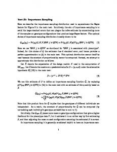
In order to deal with the nonlinearity of the model and its serial dependence, I used the E¢ cient Importance Sampling (hereafter EIS) procedure proposed by Richard and Zhang [37]. The EIS procedure is a Monte Carlo (MC) technique used for the evaluation of highdimensional integrals. It relies upon a sequence of low-dimensional regressions to construct an auxiliary MC sampler, which produces highly accurate MC estimates of the likelihood. I programmed the same procedure that Liesenfeld and Richard [31] used to estimate the SV model for daily data of IBM stock prices, S&P 500 price indexes, and the exchange rate for the US Dollar and the Deutsche Mark. The procedure is summarized below. Let rt ; t : 1 ! T is an n-dimensional vector of observable random variables and
t
is
a q-dimensional vector of latent variables. The ML procedure is based on the marginalized likelihood function L( ; R) = where R = frt gTt=1 ,
= f t gTt=1 and
Z
(1.8)
f (R; ; )d
is an unknown parameter vector. Equation (8) can
be factorized as follows Z Y T L( ; R) = f (rt ;
t
t=1
where Rt = fr gt =1 and of
t 1
t
=f
j
t 1 ; Rt 1 ;
gt =1 .The model implicitly assumes that rt is independent
conditional on ( t ; Rt 1 ) with a density of g(rt j
conditional density of p(
t
j
(1.9)
)d
t 1 ; Rt 1 ;
Z Y T L( ; R) = g(rt j
t ; Rt 1 ;
) and that
t
has the
). Whence, the likelihood can be written as t ; Rt 1 ;
)p(
t=1
t
j
t 1 ; Rt 1 ;
(1.10)
)d
The EIS procedure constructs a sequence of samplers that exploits the sample information on the
0 ts
as conveyed by rt0 s. Let, fm(
t
j
t 1 ; at )g
denotes such a sequence of (i)
auxiliary samplers indexed by the auxiliary parameters A = fat gTt=1 . Let f notes a trajectory drawn from the sequence of auxiliary samplers. Let a(t
1)
t
(at )gTt=1 de-
= fas gts=11 : The
corresponding MC estimate of the likelihood can be written as 8 (i) T >
> :t=1
fit (j) (ait )
(j)
(j) rit ; fit (ait )jRit 1 ; ] it 1 (ait 1 );
i
(j)
(j) m fit (ait )j ] it 1 (ait 1 ); ait
T
9 > > =
(3.8)
> > ;
denotes a trajectory drawn from the auxiliary samplers m ( ) :
t=1
EIS aims at selecting values of fait gTt=1 which provides a good match between the denominator and nominator in Equation 7 which will minimize the MC sampling variance of Lf N . To achieve the minimization, EIS constructs a functional approximation k ( for the conditional joint density which is analytically integrable with respect to it j
m(
it 1 ; ait )
(
Then
is given by
m( where
it :
it ; ait )
it 1 ; ait )
=
R
k(
it j
it 1 ; ait )
it ; ait ) d it .
=
Since
(
k ( it ; ait ) ( it 1 ; ait ) it 1 ; ait )
(3.9)
does not depend on
it
it can be
transferred back into the period t-1 minimization subproblem. Therefore, the problem turns back into solving a simple back-recursive sequence of low-dimensional least squares problem of the form
abt ( ) = arg min at
:
for t : T ! 1, with
(
N X
[(ln f
j=1
(j)
fit ; b ait+1 ]
iT ; aiT +1 )
(j)
(j)
rit ; fit ( )jRit 1 ; ] it 1 ( ); cit
i
(3.10)
(j) ln k fit ; b ait )2
1 and cit ’s are unknown constants to be estimated jointly
with the ait ’s. Nevertheless, in order to produce maximally e¢ cient importance samplers just a small number of EIS iterations is required. To provide the convergence of auxiliary parameters b ait ,
we apply Common Random Numbers (CRNs) technique. Finally, the ML-EIS estimates of
are obtained by maximizing Equation 7 with respect
to : 36
A detailed implementation of EIS for the SV model in Section 4 is given in Appendix.
3.2.3
The Return Variable
As mentioned earlier, in this paper we use 35 di¤erent S&P 500 stock returns from six di¤erent sectors. We investigated the e¤ect of lagged values of di¤erent return variables on volatility. For example, we tried the …rst lag of the deviation of return from its mean to the volatility equation. Moreover, we tried using the deviation of return from its monthly moving average as well as its absolute value. To compare the e¤ect of these variables on the model, we utilized the following procedures for each di¤erent extra variable candidate 1) We regress the …ltered volatilities of an individual stock return on its …rst-order lag and calculated the residuals for this estimation. 2) We regress the …rst lag-of-return variable on the …rst-order lag of the …ltered volatilities and calculated the residuals from this regression. 3) We regress the residuals from the …rst estimation on the residuals from the second regression. These estimation results could provide the coe¢ cients of the di¤erence parameter. However, they would be based on a mis-speci…ed model because the …ltered volatilities are obtained by using the standard SV model. The comparison of these estimation results for di¤erent return-variable candidates suggests that the deviation of return from its monthly moving average, which we call the di¤erence variable, has the highest e¤ect on volatility. Tables 16, 17 and 18 show the estimation results of the …nal regression of residuals for Coca-Cola, American Express, and BristolMyers Squibb. Regression results represent that estimated coe¢ cients of …nal regression are signi…cant. This indicates a relationship between the di¤erence variable and the volatility. Furthermore, if we compare these initial results with the results of ML estimation, we see that the results are close to each other in the standard deviations as well as the point estimates. Therefore, these initial estimation results were useful to the investigation before I ran the full EIS-ML. Furthermore, this similarity between initial estimation and …nal EIS-ML results is true for all 35 stocks. 37
Next, we formulate the return variable before adding it to the volatility equation. This return variable is formulated as
xit = rit
rit
(3.11)
where rit is stock return i : 1 ! 35 and t : 1 ! T: rit represents the monthly moving average of return i at time t:We do not calculate the moving averages by using the standard moving average calculation which uses observations from t 11 to t+11. Because our moving average should depend on past values, we use observations from t-22 up to t. Furthermore, by using the moving instead of the mean average (which is used in the standard GARCH(1,1) model), we allow the mean to vary over time. Because we also tested the deviation of return from its mean when choosing the return variable, the comparison of the deviation of return from both its mean and its monthly moving average, as additional variables to the volatility equation, suggests that deviation from the monthly moving average has a stronger impact on volatility.
3.3
APPLICATIONS
For the application of the model, we use 35 di¤erent daily S&P 500 stock prices form six di¤erent sectors between January 2nd 1990 and October 31st 2008. The model is estimated for Coca-Cola, Hershey, Proctor & Gamble and Walmart from the consumer staples sector; Chevron, Sunoco, ConocoPhillips and Exxon from the energy sector; American Express, Bank of America, CitiBank, JP Morgan and Wells Fargo from the …nance sector; Abbott, Amgen, Bristol-Myers Squibb, Johnson & Johnson, Merck, P…zer, Schering & Plough and Wyeth from the health sector; 3M, Boeing, Caterpillar, GE, Masco and Southwest Airlines from the industrials sector; and Apple, Hewlett Packard, Intel, IBM, Micron, Motorola, Oracle and Java from the information technologies sector. Stock returns are calculated by using formula
rit = 100: ln(sit =sit 1 ) 38
(3.12)
where sit is daily stock return for return i : 1 ! 35 andt : 1 ! 4750. Table 19 through 24 in Appendix C presents the estimation results under the standard SV model and SV model with the di¤erence variable for each industry. Numbers in parentheses represent the asymptotic standard deviations. Mean and standard deviation are the parameters’means and standard deviations respectively. For the consumer staples sector, the
parameter changes between -0.02 and -0.073 and
is signi…cant for all stock returns except Hershey. Furthermore, persistence parameter increases and the standard deviation of volatility
decreases when the di¤erence variable is
added and signi…cant. For the energy sector, the di¤erence parameter changes between -0.043 and -0.102. It is signi…cant for all returns. Persistence parameter volatility
increases and standard deviation of
decreases under the proposed model.
For the …nance sector, the di¤erence parameter
has the range of (-0.048,-0.068) and is
signi…cant for all returns. In terms of the persistence parameter and the standard deviation of volatility respectively, results again indicate increase and decrease. For the health sector, the range of di¤erence parameter is similar to the energy sector, which is between -0.027 and -0.110. The di¤erence parameter is signi…cant for all stocks. The persistence parameter increases when the di¤erence variable is added. In terms of the standard deviation of volatility, there is a decrease, except in the case of Merck. For the industrials sector, the di¤erence parameter range is again similar to the energy and health sectors. It changes between -0.019 and -0.110. This sector has two stocks with insigni…cant di¤erence parameters, 3M and Masco. The persistence parameter and the standard deviation of volatility
increases
decreases when the di¤erence variable is added for
all stocks except Masco. Finally, among all sectors, the information technology sector has the widest di¤erence in parameter range. The
parameter changes between -0.004 and -0.135 and it is not signi…cant
for Apple. Furthermore, adding the di¤erence variable into the volatility equation causes an increase and decrease in the persistence parameter and standard deviation of volatility, respectively. Almost all individual estimation results indicate that the di¤erence parameter is signif39
icant, which shows that return does “Granger-cause” volatility. Moreover, when we add the di¤erence variable into the volatility equation, persistence increases and the standard deviation of volatility decreases. To represent the e¤ect of new variables on persistence, we draw the …ltered volatility graphs of Coca-Cola and Bristol-Myers Squibb. They are obtained by standard SV model estimation and the SV model with the di¤erence variable estimation (for a small period after we observe a large xt 1 , which is the di¤erence variable). Filtered volatility is the mean of volatility at time t computed by using information available on the returns up to time t-1. For Coca-Cola we observe that the 145th observation is large enough to examine the di¤erence between two …ltered volatility series from the two models. Figure 17 in Appendix D shows the …ltered volatility series of 14 points after the large di¤erence variable is observed at 145th point for Coca-Cola. For Bristol-Squibb-Myers we observe the large xt
1
at the
1892nd observation. Figure 18 in Appendix D also represents the …ltered volatility series of 13 points after the 1892nd point by using respectively the standard SV model and the SV model with the di¤erence variable for Bristol- Myers Squibb.. Since the coe¢ cient of di¤erence variable is negative when there is a large positive xt
1
we
should expect that …ltered volatilities from the SV model with the di¤erence variable should be lower than …ltered volatilities from the standard SV model. As noted for Coca-Cola, we observe a large positive xt
1
at the 145th and the 1892nd observations for Bristol-Squibb-
Myers. Starting one point ahead of these observation points, the …ltered volatilities graphs clearly represent that …ltered volatilities are lower when the di¤erence variable is added to the model. In order to summarize the e¤ects of the di¤erence variable on volatility, we compare likelihood values under two di¤erent models for each return series as a …nal test. We use a LR-test to examine if there is an improvement in the model when we add the di¤erence variable to the volatility equation. Tables 25 through 30 in Appendix D represent the likelihood values for each return series among sectors for the two models and the LR-test results. The results suggest that the model is improved and that there is causality between return and volatility except for those stocks with an insigni…cant di¤erence parameter. Table 31 in Appendix D shows the variance-covariance structure between parameters 40
among the returns for all 35 stocks. This table represents the common feedback structure of SV model parameters among 35 stocks. Furthermore, the bivariate plot of and , Figure 19 in Appendix D, also re‡ects that, when the di¤erence parameter parameter
is added, the persistence
increases.
The …nal step of this paper is a joint EIS-ML estimation. Here the parameters for each stock are assumed to be iid draws from a common four-dimensional distribution. We introduce a re-parameterization in order to avoid the problem of ’s being no larger than one, produce a more reasonable joint distribution, simplify the correlation structure, and produce neater bivariate graphs. This re-parametrization is given by
=
(3.13)
1
= ln(
1
)
= = p
1
2
As we noted above, this re-parameterization will simplify the correlation structure and simplify the common four-dimensional distribution
3.4
CONCLUSION
The standard SV model assumes that volatility is explained only by its …rst order lag. This paper presents research focused on examining the causality between return and volatility in the SV model. The causality is given by adding a return variable to the equation, which modi…es the volatility equation in the standard SV model. The choice of this return variable is carried out by examining the partial correlation between the …rst-order lag of …ltered volatilities and …rst-order lag of return variables. The examination of di¤erent return variables suggests that using the …rst-order lag of the di¤erence between return and its past monthly moving average as the return variable provides the greatest improvement in the model. 41
After analyzing 35 di¤erent S&P 500 stock returns from six di¤erent sectors (consumer staples, …nance, energy, health, industrials, and information technology), the empirical results obtained in this paper can be summarized as follows: First, the estimation results indicate that for more than 30 stocks, the di¤erence parameter is signi…cant. Furthermore, when the di¤erence variable is added to the volatility equation, the persistence parameter increases and, more importantly, the standard deviation of volatility decreases. The reduction in the standard deviation of volatility and the signi…cant di¤erence parameter together prove the existence of Granger-causality between return and volatility. Second, the examination of …ltered volatility graphs from the SV model with the di¤erence variable also shows that …ltered volatilities decrease after a high and positive observation for the di¤erence variable. Finally, the LR-test results represent that the model is improved for stocks except Hershey, 3M, Masco, P…zer, and Apple. The …nal investigation will also be done by a joint EIS-ML estimation, where the parameters for each stock are assumed to be iid draws from a common four-dimensional distribution. In order to simplify the correlation structure between parameters, a re-parameterization will be introduced.
42
BIBLIOGRAPHY
[1] Akgiray, V., "Conditional heteroscedasticity in time series of stock returns: evidence and forecasts", Journal of Business and Economic Statistics, 1989, 7, 85-93 [2] Andersen, T., Chung, H. and Sørensen, B.E., "E¢ cient method of moments estimation of a stochastic volatility model: a Monte Carlo study", Journal of Econometrics, 1999, 91, 61–87 [3] Baillie, Richard T., Bollerslev, Tim and Mikkelsen, Hans Ole, "Fractionally integrated generalized autoregressive conditional heteroskedasticity," Journal of Econometrics, Elsevier, 1996 vol. 74(1), 3-30, September [4] Berument, H., "The impact of in‡ation uncertainty on interest rates in the UK", Scottish Journal of Political Economy", 1999, 46(20), 207-18. [5] Berument, H. and Dincer,N. Nergiz, "The e¤ects of exchange rate risk on economic performance: the Turkish experience," Applied Economics, Taylor and Francis Journals, 2005, vol. 36(21), pages 2429-2441, December [6] Berument, H., Metin-Ozcan, K. and Neyapti, B., "Modelling in‡ation uncertainty using EGARCH: an application to Turkey", 2001 [7] Bluhm, H. and Yu, J., "Forecasting volatility: evidence from the German stock market", University of Auckland, 2000, working paper [8] Bollerslev, T., "Generalized autoregressive conditional heteroscedasticity", Journal of Econometrics, 1986, 31, 307-327 [9] Brunner, A.D. and Simon, D.P. , "Excess returns and risk at the long end of the treasury market: an EGARCH-M approach", The Journal of Financial Research, 1986, 14(1), 443-457 [10] Cumby, R., Figlewski, S. and Hasbrouck, J., "Forecasting volatility and correlations with EGARCH models", Journal of Derivatives1, 1993, Winter, 51-63 [11] Danielsson, Jon, "Stochastic volatility in asset prices estimation with simulated maximum likelihood," Journal of Econometrics, Elsevier, 1994, vol. 64(1-2), 375-400 43
[12] Day, T. E. and Lewis, C.M., "Stock market volatility and the information content of stock index options", Journal of Econometrics, 1992, 52, 267-287 [13] Dunis, C. L., Gavridis, M., Harris, A., Leong, S. and Nacaskul, P., "An application of genetic algorithms to high frequency trade models: a case study", Nonlinear Modelling of High Frequency Time Series (ed. C. Dunis and B. Zhou), Chichester:Wiley, 1998 [14] Engel, R. F., "Dynamic conditional correlation - a simple class of multivariate GARCH models", University of California at San Diego, Economics Working Paper Series, 200009 [15] Engel, R. F., "Autoregressive conditional heteroscedasticity with estimates of the variance of United Kingdom in‡ation", Econometrica, 1982, 50, 987-1007 [16] Fleming, J., "The quality of market volatility forecasts implied by S&P 100 index option prices", Journal of Empirical Finance, 1998, 5, 317–345 [17] Friedman, M., "Nobel lecture: in‡ation and unemployment", Journal of Political Economy, 1977, 85, 451-472 [18] Gallant, A.R., Hsieh, D. and Tauchen, G., "Estimation of stochastic volatility models with diagnostics", Journal of Econometrics, 1997, 81 (1), 159–192 [19] Geweke, J., "Comment on Bayesian analysis of stochastic volatility", Journal of Business and Economics Statistics, 1994c, 12 (4), 371–417 [20] Ghysels, E., Harvey, A.C. and Renault, E., "Stochastic Volatility", In: Maddala, G., Rao, C.R. (Eds.), Handbook of Statistics, 1996, vol. 14. Elsevier Sciences, Amsterdam. [21] Giordani, P. and Söderlind, P., "Is there evidence of pessimism and doubt in subjective distributions? A comment on abel", SIFR Research Report Series 19, Swedish Institute for Financial Research, 2003 [22] Harvey, A.C., Ruiz, E. and Shephard, N., "Multivariate stochastic variance models", Review of Economics Studies, 1994, 61, 247-264 [23] Heynen, R. C. and Kat, H.M., "Volatility prediction: a comparison of stochastic volatility, GARCH(1,1) and EGARCH(1,1) models", Journal of Derivatives 2, 1994, Summer, 50-65 [24] Hol, E. and Koopman, S. J., "Stock index volatility forecasting with high frequency data", Tinbergen Institute Discussion Papers, 2002, 02-068/4, Tinbergen Institute [25] Hu, M.Y., Jiang, C.X. and Tsoukalas, C., "The European exchange rates before and after the establishment of the European monetary system", Journal of International Financial Markets, Institutions and Money, 11997, 7, 235-253 44
[26] Jacquier, E., Polson, N.G. and Rossi, P.E., "Bayesian analysis of stochastic volatility models (with discussion)", Journal of Business and Economic Statistics, 1994, 12, 371389 [27] Jorion, P., "Predicting volatility in the foreign exchange market", Journal of Finance, 1995, 50, 507-528 [28] Kim, S., Shephard, N. and Chib, S., "Stochastic volatility: likelihood inference and comparison with ARCH models", Review of Economic Studies, 1998, 65, 361-393 [29] Krichene, N., "Modelling Stochastic Volatility with applications to stock returns", IMF Woking Paper, 2003, 03/125 [30] Liesenfeld, R. and Richard, J.F., "Classical and Bayesian analysis of univariate and multivariate stochastic volatility models", Economic Reviews, 2007, 25, 335-360 [31] Liesenfeld, R. and Richard, J.F., "Univariate and multivariate stochastic volatility models: estimation and diagnostics", Journal of Empirical Finance, 2003, 10, 505-531 [32] Melino, A. and Turnball, S.M., "Pricing foreign currency options with stochastic volatility", Journal of Econometrics, 1990, 45, 239-265 [33] Nelson, D.B., "Conditional heteroscedasticity in asset returns: a new approach", Econometrica, 1991, 59, 347-370 [34] Rich, R. and Tracy, J., "Uncertainty and labor contract durations", Review of Economics and Statistics, 2004, 86, 270-287 [35] Richard, J.F. and Zhang, W., "Econometric modeling of UK house prices using accelerated importance sampling", Oxford Bulletin of Economics and Statistics, 1996, 58, 601-613 [36] Richard, J.F. and Zhang, W., "Accelerated Monte Carlo integration: an application to dynamic latent variable models", In: Mariano, R., Weeks, M., Schuermann, T. (Eds.), "Simulation Based Inference Econometrics: Model and Application", Cambridge University Press, 1997, 47-70 [37] Richard, J.F. and Zhang, W., "E¢ cient high dimensional Monte Carlo importance sampling", Journal of Econometrics, 2007, 141, 1385-1411 [38] Takahashi, M., Omori, Y. and Watanabe, T., "Estimating stochastic volatility models using daily returns and realized volatility simultaneously", Computational Statistics&Data Analysis, 2009, 53-6, 2404-2426 [39] Taylor, S.J., "Financial returns modelled by the product of two stochastic processes-a study of daily sugar prices", In: Anderson, O.D. (Ed.), Time Series Analysis: Theory and Practice 1, North Holland, Amsterdam, 1982, 203-226 45
[40] Taylor, S.J., "Modelling Financial Time Series", Chichester:Wiley, 1986 [41] Taylor, S. J., "Modeling stochastic volatility: A review and comparative study", Mathematical Finance, 1994, 4, 183-204 [42] Tse, Y. and Booth, G.G., "Common volatility and volatility spillovers between U.S. and Eurodollar interest rates: evidence from the futures market", Journal of Economics and Business, 1996, 48, 299-312
46
APPENDIX A
IMPLEMENTATION OF EIS FOR STOCHASTIC VOLATILITY MODEL WITH DIFFERENCE PARAMETER
This appendix represents the functional forms of EIS implementation for the SV model with extra di¤erence parameter in the volatility equation given by Equation .(4): Let the integrating constant of kt (
t+1
(
ait+1 ) it ; b
it ;
= exp
ait ) it 1 ; b
1 (pit+1 2
w.r.t.
2 it
it
2qit+1
be formulated as
it
+ rit+1 )
(A.1)
where (pt+1 ; qt+1 ; rt+1 ) are the appropriate functions of the EIS auxiliary parameter b ait+1 which will be obtained by backward recursions.
= 1; values of pi ; qi and ri at T + 1
T +1
are equal to 0. Let the EIS approximation for the product of density function of return be denoted as:
kt1 (
ait ) it ; b
1 b (bit 2
= exp
2 it
2b cit
(A.2)
it )
The EIS auxiliary parameter b ait is describes as b ait = bbit ; b cit . Then the EIS kernel can
be represented as
kt (
it ;
it 1 ; ait )
= kt1 (
ait )p ( it j it ; b
it 1 ; Rit 1 ; i )
t+1
(
ait+1 ) it ; b
(A.3)
Furthermore, the conditional densities for return and volatility are de…ned as:
g (rit j
it ; Rit 1 ; i )
exp 47
1 2
it
+ rit2 exp(
it )
(A.5)
p(
it j
it 1 ; Rit 1 ; i )
1 =p exp 2vi
1 ( 2
it
2 i xit 1 )
i it 1
i
=
2 i
(A.6)
If we combine together,A.1, A.2. and A.5. we have
2 ln kt1 (
it ;
ait ) it 1 ; b
=
2 it
bbit + 1=
+(
2 i
+2
i
2 i
2 2 i it 1
+
2
2 it
2 2 i xit 1
+
+2
i
+
+
2 i xit 1 )= i (A.7)
i i
+
i i xit 1 )
2 2 i it 1
+
2 2 i xit 1 )
it 1
(
i it 1
2 i
ixit 1 )=
+pit+1
b cit + (
it
2qit+1
it
+ rit+1
I we rewrite the equation as follows
2 ln kt1 (
it ;
ait ) it 1 ; b
2 it Ait
=
2
it 1
+2
2 i i xit 1 )= i
i i
2 it
Bit = b cit + (
i
+
+
i it 1
2 i
+
it
+ rit+1
2 i
+
It immediately follows that the EIS sampler for
(A.9)
2 i xit 1 )= i it j it 1
(A.10)
is given by
N Ait 1 Bit ; Ait 1
ait ) it j it 1 ; b
(A.8)
i i xit 1 )
2qit+1
Ait = bbit + 1=
mt (
+(
+2
+pit+1
(
it Bit
(A.11)
We can obtain the log-integrating constant by re-grouping all the remaining factors in A.5 and is therefore in form introduced in A.1 together with
pit =
2 2 i= i
48
Ait
2
(A.12)
qit = (
+
i i
2 i
rit = (
2 i i xit 1 ) = i
+2
i i xit 1
(b cit +
i
+
+
Ait (b cit +
i
+
(A.13)
i xit 1 )
2 2 2 i xit 1 )= i
cit i xit 1 )Ait (b
+
(A.14) i
+
i xit 1 )
Hence equations (A.9)-(A.10) and (A.12)-(A.14) fully characterize the EIS recursion whereby the coe¢ cients (pt+1 ; qt+1 ; rt+1 ) are combined with the period t EIS coe¢ cients bbit ; b cit in order to produce (back recursively) the coe¢ cients (Ait ; Bit ) characterizing the
EIS-sampling densities.
Based on these the EIS steps can be described as follows: Step 1. Generate N independent trajectories from the initial sampler m
(0) it j it 1 ; at
Such a sequence can be found by e.g. using a Taylor Series Approximation (TSA) in
it
.
for
conditional density of return around its mean which is equal to zero. Replacing the resulting TSA values with bbit ; b cit in equations (A.9) and (A.10) provides the initial samplers together
with the recursions described above.
Step 2. Now we can use these trajectories for solving the back recursive LS problem de…ned in Equation 12. This requires to run for each period t the following linear regression
where
(i) it
ln g rit j fit
(i)
= constant
represents the regression error term.
(i) 1 e(i)2 bit it + cit eit + 2
(i) it
(15)
Step 3. Use the LS estimates bbit and b cit obtained in Step 2 to construct back-recursively
the sequence of EIS-sampling densities as given by Equation (A.11) together with the recursions (A.9)-(A.10) and (A.12)-(A.14).
Step 4. Use N independent trajectories from auxiliary samplers constructed in Step 3 and then repeat Step 2 and 3 to compute EIS-MC estimate of the likelihood function. 49
APPENDIX B
FIGURES AND TABLES OF CHAPTER 1
Turkey's Inflation 30
Inflation Rate
25 20 15 10 5 0 -5
1
18 35 52 69 86 103 120 137 154 171 188 205 222 239 256 273 Number of Observations
Figure 1: In‡ation Series of Turkey
50
Detrended Turkey's Inflation 25
Inflation Rate
20 15 10 5 0 -5
1
20 39
58 77 96 115 134 153 172 191 210 229 248 267
-10 Nmber of Observ ations
Figure 2: The Detrended and Deseasonalized In‡ation Series of Turkey.
Figure 3: Filtered Volatilities from EGARCH Model (GED) without Dummies
51
Figure 4: Filtered Volatilities tiwh EGARCH Model without dummies
Figure 5: Filtered Volatilities with SV Model without Dummies
52
Figure 6: Filtered Volatilitilies from EGARCH (GED) Model with Dummies
Figure 7: Filtered Volatilities from EGARCH Model with Dummies
53
Figure 8: Filtered Volatilities from SV Model with Dummies
Coe¢ cients t-statistics P-value In‡ation(-1) 0:341
7:720
0:000
1:146
3:966
0:000
January February
0:694
2:376
0:018
March
0:161
0:571
0:568
April
0:445
1:542
0:124
May
0:994
3:452
0:000
June
1:775
6:358
0:000
July
1:061
3:589
0:000
August
0:324
1:108
0:268
September
1:546
5:296
0:000
October
1:471
5:011
0:000
November
0:023
0:076
0:939
December R-squared
0:584
2:014
0:045
0:623
Table 1: Regression of Turkey’s In‡ation on Monthly Dummies before Seasonal Adjustment
54
Coe¢ cients t-statistics P-value In‡ation(-1) 0:361
8:344
0:000
January
0:093
0:348
0:727
February
0:325
1:215
0:225
March
0:141
0:539
0:590
April
0:187
0:698
0:485
May
0:293
1:108
0:268
June
0:134
0:511
0:609
July
0:111
0:423
0:672
August
0:052
0:198
0:842
September
0:081
0:304
0:761
October
0:011
0:042
0:966
November
0:112
0:418
0:675
December
0:369
R-squared
0:510
1:377
0:169
Table 2: Regression of In‡ation Series of Turkey on Monthly Dummies after Seasonal Adjustment
55
Coe¢ cients P-value In‡ation(-1) 0 1
0:4716 0:1888 0:5083
0:000 0:071 0:018
2
0:1452
0:042
3
0:0902
0:043
4
Log-likelihood
0:8912
0:000
441:27
Table 3: EGARCH (GED) Results without Dummy Variables
Coe¢ cients P-value In‡ation(-1)
0:319
0:000
DUMMY1
4:608
0:625
DUMMY2
8:009
0:033
DUMMY3
18:515
0:000
DUMMY4
1:514
0:010
0
0:032
0:917
1
0:257
0:182
2
0:082
0:708
3
0:191
0:112
4
Log-likelihood
0:497
0:230
413:03
Table 4: EGARCH (GED)Results with Dummy Variables
56
Coe¢ cients P-value In‡ation(-1) 0 1
0:4818 0:1610 0:4530
0:000 0:070 0:012
2
0:1094
0:511
3
0:0753
0:396
4
Log-likelihood
0:8883
0:000
436:56
Table 5: EGARCH Results without Dummy Variables
Coe¢ cients P-value In‡ation(-1)
0:392
0:000
DUMMY1
4:848
0:007
DUMMY2
7:820
0:041
DUMMY3
18:797
0:000
DUMMY4
3:387
0:069
0
1
0:076 0:324
0:427 0:153
2
0:110
0:640
3
0:105
0:290
4
Log-likelihood
0:908
0:000
396:02
Table 6: EGARCH Results with Dummy Variables
57
Coe¢ cients Asympt. stand. err. MC stand. err. 0:0465
Log-likelihood
0:03
0:0005
0:8160
0:05
0:0007
0:4506
0:09
0:0023
380:53
0:0640
Table 7: SV Model Results without Dummy Variables
Coe¢ cients Asympt stand. err. MC stand. err. 1
3:8465
1:05
0:0002
2
0:1554
0:82
0:0002
3
0:0859
1:26
0:0001
4
2:2106
0:87
0:0004
0:0569
Log-likelihood
0:05
0:0005
0:8531
0:85
0:0006
0:4357
0:43
0:0021
374:95
0:053
Table 8: SV Model Results with Dummy Variables
58
In‡ation Skewness 0:3486 Kurtosis
3:1956
KS(z )
0:0505
Q30 (z )
183:56
Q30 (z)
160:13
(0:23)
(0:00)
(0:00)
2
Q30 (z )
3:15
(1:00)
Q30 (z 2 )
26:226 (0:66)
Table 9: Results for Diagnostic Checks
59
APPENDIX C
FIGURES AND TABLES OF CHAPTER 2
US Inflation 0.3 0.25
Inflation Rate
0.2 0.15 0.1 0.05
0 -0.05 1
90
179 268 357 446
535 624 713 802 891 980 1069
-0.1 -0.15 -0.2 Number of Observations
Figure 9: U.S. In‡ation Series
60
US Inflation After AR(1) 0.08
Inflation Rate
0.06 0.04 0.02 0
-0.02
1
75
149 223 297 371 445 519 593 667 741 815 889 963 1037 1111
-0.04 -0.06 Number of Observations
Figure 10: Graph of U.S In‡ation Series after Autocorrelation is Eliminated
Cumulative Distribution for US
Probability
1 0.9 0.8 0.7 0.6 0.5 0.4 0.3 0.2 0.1 0 1 16 31 46 61 76 91 106 121 136 151 166 181 196 211 226 241 256 271 286 301 316 Number of Observations
Figure 11: Cumulative Empricial Distribution Graph for U.S.
61
Turkey's Inflation 30 25
Inflation Rate
20 15 10 5 0 -5
1
18 35 52 69 86 103 120 137 154 171 188 205 222 239 256 273 Number of Observations
Figure 12: In‡ation Series of Turkey
Detrended Turkey's Inflation 25
Inflation Rate
20 15 10 5 0 -5
1
20 39
58 77 96 115 134 153 172 191 210 229 248 267
-10 Nmber of Observ ations
Figure 13: The Detrended In‡ation Series of Turkey.
62
After Seasonal Adjusment 20
Inflation Rate
15 10 5 0 1
21
41
61
81 101 121 141 161 181 201 221 241 261 281
-5 -10 Number of Observ ations
Figure 14: In‡ation Series of Turkey after Seasonal Adjustment.
Turkey's Inflation After AR(1) 4 3
Inflation Rate
2 1
0 -1 1
15 29 43 57 71 85 99 113 127 141 155 169 183 197 211 225 239 253 267 281
-2 -3 -4 -5 Number of Observations
Figure 15: In‡ation Series of Turkey after Autocorrelation is Eliminated.
63
Cumulative Distribution for Turkey 1.2
Probability
1 0.8 0.6 0.4 0.2 0 1 4 7 10 13 16 19 22 25 28 31 34 37 40 43 46 49 52 55 58 61 64 67 70 73 76 79 82 Number of Observations
Figure 16: Cumulative Empricial Distribution Graph for Turkey.
Student-t distribution 1
Probabilitity
0.9 0.8 0.7 0.6 0.5 0.4 0.3 0.2 0.1 0 1
5
9 13 17 21 25 29 33 37 41 45 49 53 57 61 65 69 73 77 81 Number of observations
Figure 17: Cumulative Distribution Graph for the First Simulated Series by Using Student-t Distribution.
Coe¢ cients Asymptotic Std. Err. MC Std. Err. 0:0012
0:004
0:0001
0:9911
0:005
0:0004
0:1986
0:042
0:0021
Table 10: Initial SV Model Estimation Results for U.S
64
Coe¢ cients Asymptotic Std. Err. MC Std. Err. 0:0007
0:003
0:0001
0:9918
0:004
0:0003
0:2108
0:035
0:0018
Table 11: Final SV Model Estimation Results for U.S
Coe¢ cients t-statistics p-value In‡ation(-1) 0:357
6:290
0:000
1:173
3:118
0:002
January February
0:691
1:816
0:070
March
0:210
0:572
0:567
April
1:283
3:490
0:000
May
0:972
2:591
0:013
June
1:726
4:679
0:000
July
0:990
2:583
0:000
August
0:258
0:679
0:497
September
1:587
4:184
0:000
October
1:476
3:861
0:000
November
0:016
0:040
0:967
December R-squared
0:573
1:518
0:130
0:369
Table 12: Regression of Turkey’s In‡ation on Monthly Dummies before Seasonal Adjustment
65
Coe¢ cients t-statistics p-value In‡ation(-1) 0:101
1:682
0:093
January
0:071
0:178
0:858
February
0:280
0:699
0:485
0:126
0:899
March
0:050
April
0:021
May
0:054
0:510
1:302
0:956 0:194
June
0:000
0:000
0:999
July
0:050
0:128
0:897
August
0:855
2:184
0:029
September
0:004
0:011
0:091
October
0:094
0:234
0:814
November
0:704
1:760
0:79
December R-squared
0:321
0:803
0:422
0:045
Table 13: Regression of Turkey’s In‡ation on Monthly Dummies after Seasonal Adjustment
Coe¢ cients Asymptotic Std. Err. MC Std. Err. 0:0402
0:031
0:0007
0:7655
0:052
0:0009
0:4939
0:091
0:0035
Table 14: Intial SV Model Estimation Results for Turkey
66
Coe¢ cients Asymptotic Std. Err. MC Std. Err. 0:0572
0:025
0:0006
0:8792
0:036
0:0007
0:4457
0:077
0:0031
Table 15: Final SV Model Estimation Results for Turkey
67
APPENDIX D
FIGURES AND TABLES OF CHAPTER 3
CocaCola Filtered Volatility
1.6 1.4 1.2 1 0.8 0.6 0.4 0.2 0 1
2
3
4
5
6
7
8
9
10
11
12
13
14
Number of Data point SV with diff.param.
Standard SV
Figure 18: Filtered Volatility Series for CocaCola
68
Bristol&Squibb&Myers 0.8
Filtered Volatility
0.6 0.4 0.2 0 -0.2
1
2
3
4
5
6
7
8
9
10
11
12
13
-0.4 -0.6 Num ber of Data Standard SV
SV w ith diff. param.
Figure 19: Filtered Volatility Series for Bristol-Squibb-Myers.
Bivariate Plot of Delta and Beta 1.2 1
Delta
0.8 0.6 0.4 0.2 0 -0.15
-0.1
-0.05
0
Beta
Figure 20: Bivariate Plot of Delta and Beta for 35 Stocks
Results for Final Regression Coe¢ cient Standard Dev. residuals-reg2 R-squared
0:021
0:003
0:153
Table 16: Estimation Results of Residual Regression for CocaCola
69
Results for Final Regression Coe¢ cient Standard Dev. residuals-reg2 R-squared
0:010
0:002
0:181
Table 17: Estimation Results of Residual Regression for American Express
Results for Final Regression Coe¢ cient Standard Dev. residuals-reg2 R-squared
0:019
0:004
0:194
Table 18: Estimation Results of Residual Regression for Bristol-Squibb-Myers
Standard SV Model
SV Model with Di¤erence Var.
Stocks CocaCola
0:009 (0:003)
Hershey
0:057 (0:011)
Proctor & Gamble
0:015 (0:004)
Walmart
0:001 (0:001)
Mean Standard Deviation
0:020 0:025
0:982
(0:0045)
0:904
(0:0152)
0:973
(0:0064)
0:990
0:166
(0:0176)
0:381
(0:0325)
0:196
(0:0215)
0:104
(0:0031)
(0:0142)
0:962
0:212
0:039
0:119
0:007 (0:0030)
0:058 (0:0108)
0:014 (0:0049)
0:000
(0:0013)
0:020 0:026
0:986
(0:0041)
0:904
(0:0152)
0:976
(0:0066)
0:993
(0:0025)
0:965 0:039
0:073 (0:0126)
0:020 (0:0182)
0:059 (0:0149)
0:054 (0:0101)
0:062 0:020
Table 19: Estimation Results for Consumer Staples Sector
70
0:146
(0:0175)
0:382
(00319)
0:182
(0:0240)
0:089
(0:0123)
0:199 0:119
Standard SV Model
SV Model with Di¤erence Var.
Stocks Chevron
0:015 (0:0050)
Sunoco
0:009 (0:0039)
ConocoPhillips
0:012 (0:0041)
Exxon
0:014
0:980
(0:0058)
0:966
(0:0086)
0:973
(0:0086)
0:983
0:126
(0:0159)
0:192
(0:0252)
0:137
(0:0187)
0:129
0:012 (0:0041)
0:007 (0:0034)
0:010 (0:0035)
0:011
0:984
(0:0047)
0:973
(0:0077)
0:976
(0:0063)
0:986
(0:0049)
(0:0050)
(0:0161)
Mean
-0:020
0:962
0:211
0:019
0:980
Standard Deviation
0:025
0:039
0:119
0:026
0:006
(0:0041)
(0:0042)
0:096 (0:0141)
0:043 (0:0121)
0:067 (0:0126)
0:102 (0:0145)
0:077 0:027
0:107
(0:0137)
0:170
(0:0250)
0:125
(0:0162)
0:113
(0:0142)
0:129 0:028
Table 20: Estimation Results for Energy Sector
Standard SV Model
SV Model with Di¤erence Var.
Stocks American Express
0:003 (0:0024)
Bank of America
0:006 (0:0030)
CitiBank
0:006 (0:0028)
JP Morgan
0:003 (0:0022)
Wells Fargo
0:000
0:986
(0:0034)
0:986
(0:0035)
0:989
(0:0031)
0:988
(0:0033)
0:993
0:154
(0:0164)
0:178
(0:0166)
0:147
(0:0157)
0:155
(0:0167)
0:124
0:002 (0:0022)
0:005 (0:0032)
0:002 (0:0018)
0:001 (0:0022)
0:000
0:989
(0:0031)
0:989
(0:0036)
0:995
(0:0010)
0:992
(0:0032)
0:996
(0:0015)
(0:0026)
(0:0140)
(0:0012)
(0:0012)
Mean
0:004
0:988
0:152
0:002
0:992
Standard Deviation
0:003
0:003
0:019
0:002
0:003
Table 21: Estimation Results for Finance Sector
71
0:053 (0:0115)
0:050 (0:0104)
0:069 (0:0127)
0:049 (0:0099)
0:052 (0:0098)
0:054 0:008
0:138
(0:0158)
0:167
(0:0166)
0:122
(0:0145)
0:139
(0:0159)
0:110
(0:0119)
0:135 0:021
Standard SV Model
SV Model with Di¤erence Var.
Stocks Abbott
0:019 (0:0054)
Amgen
0:004
(0:0034)
Bristol&Squibb&Myers
0:018 (0:0052)
Johnson&Johnson
0:017 (0:0049)
Merck
0:072 (0:0140)
P…zer
0:002 (0:0026)
Schering&Plough
0:011 (0:0041)
Wyeth
0:018 (0:0051)
0:968
(0:0079)
0:965
(0:0069)
0:970
(0:0062)
0:980
(0:0045)
0:874
(0:0201)
0:970
(0:0063)
0:963
(0:0074)
0:968
0:182
(0:0222)
0:227
(0:0210)
0:213
(0:0207)
0:165
(0:0167)
0:392
(0:0322)
0:178
(0:0182)
0:226
(0:0216)
0:231
(0:0069)
(0:0235)
Mean
0:019
0:957
0:226
Standard Deviation
0:023
0:034
0:071
0:017 (0:0054)
0:001
(0:0037)
0:017 (0:0052)
0:014 (0:0046)
0:072 (0:0013)
0:001 (0:0027)
0:010 (0:0043)
0:015 (0:0051)
0:018 0:023
0:969
(0:0076)
0:966
(0:0066)
0:972
(0:0063)
0:985
(0:0040)
0:875
(0:0178)
0:972
(0:0064)
0:966
(0:0074)
0:971
(0:0067)
0:048 (0:0117)
0:062 (0:0159)
0:110 (0:0158)
0:038 (0:0173)
0:028 (0:0119)
0:046 (0:0131)
0:047 (0:0151)
0:179
(0:0220)
0:224
(0:0205)
0:207
(0:0215)
0:147
(0:0159)
0:392
(0:0318)
0:174
(0:0186)
0:216
(0:0236)
0:223
(0:0237)
0:960
0:053
0:220
0:035
0:048
0:075
Table 22: Estimation Results for Health Sector
72
0:045 (0:0159)
Standard SV Model
SV Model with Di¤erence Var..
Stocks 3M
0:092 (0:0173)
Boeing
0:022 (0:0066)
Caterpillar
0:028 (0:0073)
GE
0:073 (0:0064)
Masco
0:031 (0:0084)
Southwest Airlines Mean Standard Deviation
0:007
0:906
(0:0161)
0:946
(0:0109)
0:903
(0:0174)
0:991
(0:0071)
0:913
(0:0154)
0:933
0:348
(0:0330)
0:262
(0:0293)
0:313
(0:0320)
0:134
(0:0150)
0:363
(0:0340)
0:262
(0:0037)
(0:0119)
(0:0262)
0:040
0:932
0:280
0:033
0:083
0:036
0:089 (0:0164)
0:018 (0:0062)
0:026 (0:0068)
0:004 (0:0023)
0:031 (0:0079)
0:006
(0:0040)
0:027 0:033
0:909
(0:0154)
0:956
(0:0108)
0:911
(0:0172)
0:994
(0:0023)
0:913
(0:0137)
0:934
(0:0122)
0:936 0:034
Table 23: Estimation Results for Industrials Sector
73
0:027 (0:0226)
0:059 (0:0142)
0:036 (0:0151)
0:110 (0:0128)
0:020 (0:0158)
0:041 (0:0124)
0:049 0:033
0:343
(0:0312)
0:233
(0:0293)
0:300
(0:0303)
0:096
(0:0124)
0:364
(0:0335)
0:260
(0:0260)
0:266 0:097
Standard SV Model
SV Model with Di¤erence Var.
Stocks Apple
0:083 (0:0158)
Hewlett Packard
0:055 (0:0110)
Intel
0:014 (0:0042)
IBM
0:055 (0:0119)
Micron
0:001 (0:0012)
Motorola
0:041 (0:0091)
Oracle
0:009 (0:0041)
Java
0:013 (0:0050)
Mean Standard Deviation
0:034 0:029
0:831
(0:0260)
0:941
(0:0102)
0:982
(0:0050)
0:964
(0:0072)
0:992
(0:0011)
0:950
(0:0094)
0:974
(0:0060)
0:948
0:460
(0:0411)
0:298
(0:0264)
0:143
(0:0175)
0:242
(0:0229)
0:121
(0:0213)
0:278
(0:0258)
0:222
(0:0227)
0:258
(0:0104)
(0:0275)
0:948
0:253
0:050
0:104
0:083 (0:0154)
0:054 (0:0104)
0:011 (0:0038)
0:045 (0:0106)
0:000
(0:0012)
0:038 (0:0083)
0:007 (0:0036)
0:011 (0:0048)
0:031 0:029
0:830
(0:0232)
0:943
(0:0093)
0:984
(0:0044)
0:970
(0:0063)
0:994
(0:0024)
0:953
(0:0086)
0:980
(0:0051)
0:953
(0:0099)
0:951 0:052
0:004 (0:0172)
0:061 (0:0206)
0:075 (0:0144)
0:136 (0:0236)
0:018 (0:0089)
0:064 (0:0181)
0:084 (0:0132)
0:042 (0:0141)
0:060 0:041
0:461
(0:0339)
0:294
(0:0243)
0:130
(0:0168)
0:222
(0:0217)
0:081
(0:0118)
0:269
(0:0246)
0:193
(0:0217)
0:245
(0:0262)
0:237 0:115
Table 24: Estimation Results for Information Technology Sector
Stocks
LL-standard SV LL-SV with di¤. variable. LR-test
CocaCola
5702:28
5686:27
32:02
Hershey
5707:99
5707:82
0:34
Proctor & Gamble
5569:58
5561:93
15:30
Walmart
6676:04
6661:91
28:26
Table 25: Log-likelihood Values for Consumer Staples Sector
74
Stocks
LL-standard SV LL-SV with di¤. variable LR-test
Chevron
4995:70
4976:32
38:76
Sunoco
6309:99
6304:99
10:00
ConocoPhillips
5794:81
5780:93
27:76
Exxon
4800:30
4783:99
32:62
Table 26: Log-likelihood Values for Energy Sector
Stocks
LL-standard SV LL-SV with di¤. variable LR-test
American Express
6315:69
6305:30
20:78
Bank of America
5741:38
5731:06
20:64
CitiBank
5380:22
5365:51
29:42
JP Morgan
6496:49
6484:86
23:26
Wells Fargo
6373:22
6359:97
26:50
Table 27: Log-likelihood Values for Finance Sector
Stocks
LL-standard SV LL-SV with di¤. variable LR-test
Abbott
5589:03
5576:97
24:12
Amgen
7105:79
7089:53
32:52
Bristol-Squibb-Myers
5488:35
5480:90
14:9
Johnson & Johnson
4739:49
4718:44
42:1
Merck
5757:24
5745:73
23:02
P…zer
6770:65
6769:82
1:66
Schering & Plough
6276:21
6267:47
17:48
Wyeth
5735:63
5729:87
11:52
Table 28: Log-likelihood Values for Health Sector
75
Stocks
LL-standard SV LL-SV with di¤. variable LR-test
3M
4760:24
4760:26
0:04
Boeing
6020:08
6011:91
16:34
Caterpillar
6356:55
6344:68
23:74
GE
5083:66
5050:75
65:82
Masco
6287:67
6287:64
0:06
Southwest Airlines
7232:27
7225:22
14:1
Table 29: Log-likelihood Values for Industrials Sector
Stocks
LL-standard SV LL-SV with di¤. variable LR-test
Apple
6018:50
6018:76
0:52
Hewlett Packard
4826:30
4822:72
7:16
Intel
5154:83
5146:88
15:9
IBM
3351:23
3338:70
25:06
Micron
7021:04
7001:44
39:2
Motorola
5126:90
5120:51
12:78
Oracle
6098:83
6080:89
35:88
Java
6437:10
6424:80
24:6
Table 30: Log-likelihood Values for Information Technology Sector
76
0:00065 0:00065
0:00140
0:00011
0:00058 0:00079
0:00158
0:00335 0:00137 0:00889
Table 31: Variance-Covariance Matrix of Model Parameters
77