APPLYING MACHINE LEARNING ALGORITHMS IN SOFTWARE DEVELOPMENT Du Zhang Department of Computer Science California State University Sacramento, CA 95819-6021
[email protected] Abstract Machine learning deals with the issue of how to build programs that improve their performance at some task through experience. Machine learning algorithms have proven to be of great practical value in a variety of application domains. They are particularly useful for (a) poorly understood problem domains where little knowledge exists for the humans to develop effective algorithms; (b) domains where there are large databases containing valuable implicit regularities to be discovered; or (c) domains where programs must adapt to changing conditions. Not surprisingly, the field of software engineering turns out to be a fertile ground where many software development tasks could be formulated as learning problems and approached in terms of learning algorithms. In this paper, we first take a look at the characteristics and applicability of some frequently utilized machine learning algorithms. We then provide formulations of some software development tasks using learning algorithms. Finally, a brief summary is given of the existing work. Keywords: machine learning, software engineering, learning algorithms. 1.
The Challenge
The challenge of modeling software system structures in a fastly moving scenario gives rise to a number of demanding situations. First situation is where software systems must dynamically adapt to changing conditions. The second one is where the domains involved may be poorly understood. And the last but not the least is one where there may be no knowledge (though there may be raw data available) to develop effective algorithmic solutions. To answer the challenge, a number of approaches can be utilized [1,12]. One such approach is the transformational programming. Under the transformational programming, software is developed, modified, and maintained at specification level, and then automatically transformed into production-quality software through automatic program synthesis [5]. This software development paradigm will enable software engineering to become the discipline of capturing and automating currently undocumented domain and design knowledge [10]. Software engineers will deliver knowledge-based application generators rather than unmodifiable application programs. In order to realize its full potential, there are tools and methodologies needed for the various tasks inherent to the transformational programming. In this paper, we take a look at how machine learning (ML) algorithms can be used to build tools for software development and maintenance tasks. The rest of the paper is organized as follows. Section 2 provides an overview of machine learning and frequently used learning algorithms. Some of the software development and maintenance tasks for which learning algorithms are applicable are given in Section 3. Formulations of those tasks in terms of the learning
algorithms are discussed in Section 4. Section 5 describes some of the existing work. Finally in Section 6, we conclude the paper with remarks on future work. 2.
Machine Learning Algorithms
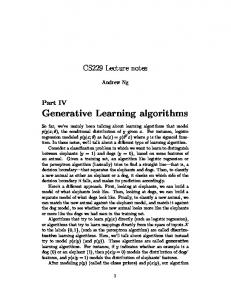
Machine learning deals with the issue of how to build computer programs that improve their performance at some task through experience [11]. Machine learning algorithms have been utilized in: (1) data mining problems where large databases may contain valuable implicit regularities that can be discovered automatically; (2) poorly understood domains where humans might not have the knowledge needed to develop effective algorithms; and (3) domains where programs must dynamically adapt to changing conditions [11]. Learning a target function from training data involves many issues (function representation, how and when to generate the function, with what given input, how to evaluate the performance of generated function, and so forth). Figure 1 describes the dimensions of the target function learning. Major types of learning include: concept learning (CL), decision trees (DT), artificial neural networks (ANN), Bayesian belief networks (BBN), reinforcement learning (RL), genetic algorithms (GA) and genetic programming (GP), instance-based learning (IBL), inductive logic programming (ILP), and analytical learning (AL). Table 1 summarizes the main properties of different types of learning. Not surprisingly, machine learning methods can be (and some have already been) used in developing better tools or software products. Our preliminary study identifies the software development and maintenance tasks in the following areas to be appropriate for machine learning applications: requirement engineering (knowledge elicitation, prototyping); software reuse (application generators); testing and validation; maintenance (software understanding); project management (cost, effort, or defect prediction or estimation). 3.
Software Engineering Tasks
Table 2 contains a list of software engineering tasks for which ML methods are applicable. Those tasks belong to different life-cycle processes of requirement specification, design, implementation, testing and maintenance. This list is by no means a complete one. It only serves as a harbinger of what may become a fertile ground for some exciting research on applying ML techniques in software development and maintenance. One of the attractive aspects of ML techniques is the fact that they offer an invaluable complement to the existing repertoire of tools so as to make it easier to rise to the challenge of the aforementioned demanding situations. 4.
Applying ML Algorithms to SE Tasks
In this section, we formulate the identified software development and maintenance tasks as learning problems and approach the tasks using machine learning algorithms. Component reuse Component retrieval from a software repository is an important issue in supporting software reuse. This task can be formulated into an instance-based learning problem as follows:
convergence
conditions
settings
feasibility
evaluating hypotheses
hypotheses comparison
confidence intervals knowledge compilation
local minima
training data property
random error
global
local
approximation
noisy/accurate
rote
justification
probabilistic
logical
generalization time
valuation
vector value
real value
discrete value
Horn clauses
propositions
linear functions
bayesian networks
decision trees
ANN
bit string/programs
attribute constraints
formalism
eager
lazy
implicit
explicit
representation
statistical
unsupervised
supervised
supervision
B + small set clauses
FOIL_gain
similarity to NN
small/large
D+B
cases
fitness
small trees
c contained in H
inductive bias
Figure 1. Dimensions of learning.
crowding
dimensionality
curse of
practical problem
augmentation
overfitting
no explicit search
randomized beam
knowledge
m-esti. accuracy
form of learning
mistake bound
analysis framework
(sample/true error)
PAC
(inductive+analytic)
hybrid
relat. frequency
simpleTocomplex deductive
-subset of
-all cases
D alone
domain theory
greedy (hill clim.)
generate/test
generalTospecific
search in H
cumulat. reward
fitness
gradient desce.
distance metric
info. gain
VS
guiding factor for search
instance-based (CBR)
reinforcement
GA/GP
decision trees
Bayesian BN
ILP
ANN
analytic (EBL)
hypothesis accuracy
changing conditions in domains
poorly understood domains
data mining
application types
learning types
target function learning
Table 1. Major types of learning methods1.
1 2 3
Type
Target function
Target function generation2
Search
Inductive bias
Algorithm3
AL
Horn clauses
Eager, supervised, D+B
Deductive reasoning
B + set of Horn clauses
Prolog-EBG
ANN
ANN
Eager, supervised, D (global)
Gradient descent guided
Smooth interpolation between data points
Backpropagation
BBN
Bayesian network
Eager, supervised, D (global), explicit or implicit
Probabilistic, no explicit search
Minimum description length
MAP, BOC, Gibbs, NBC
CL
Conjunction of attribute constraints
Eager, supervised, D (global)
Version Space (VS) guided
c∈H
Candidate_ elimination
DT
Decision trees
Eager, supervised, D (global)
Information gain (entropy)
Preference for small trees
ID3, C4.5, Assistant
GA GP
Bit strings, program trees
Eager, unsupervised, no D
Hill climbing (simulated evolution)
Fitness-driven
Prototypical GA/GP algorithms
IBL
Not explicitly defined
Lazy, supervised, D (local)
Statistical reasoning
Similarity to NN
K-NN, LWR, CBR
ILP
If-then rules
Eager, supervised, D (global)
Statistical, general-tospecific
Rule accuracy, FOIL-gain, shorter clauses
SCA, FOIL, inverse resolution
RL
Control strategy π*
Eager, unsupervised, no D
Through training episodes
Actions with max. Q value
Q, TD
The classification here is based on materials in [11]. The sets D and B refer to training data and domain theory, respectively. The algorithms listed are only representatives from different types of learning.
Table 2. SE tasks and applicable ML methods. SE tasks
Applicable type(s) of learning
Requirement engineering
AL, BBN, LL, DT, ILP
Rapid prototyping
GP
Component reuse
IBL (CBR4)
Cost/effort prediction
IBL (CBR), DT, BBN, ANN
Defect prediction
BBN
Test oracle generation
AL (EBL5)
Test data adequacy
CL
Validation
AL
Reverse engineering
CL
1. Components in a software repository are represented as points in the n-dimensional Euclidean space (or cases in a case base). 2. Information in a component can be divided into indexed and unindexed information (attributes). Indexed information is used for retrieval purpose and unindexed information is used for contextual purpose. Because of the curse of dimensionality problem [11], the choice of indexed attributes must be judicious. 3. Queries to the repository for desirable components can be represented as constraints on indexable attributes. 4. Similarity measures for the nearest neighbors of the desirable component can be based on the standard Euclidean distance, distance-weighted measure, or symbolic measure. 5. The possible retrieval methods include: K-Nearest Neighbor, inductive retrieval, Locally Weighted Regression. 6. The adaptation of the retrieved component for the task at hand can be structural (applying adaptation rules directly to the retrieved component), or derivational (reusing adaptation rules that generated the original solution to produce a new solution). Rapid prototyping Rapid prototyping is an important tool for understanding and validating software requirements. In addition, software prototypes can be used for other purposes such as user training and system testing [18]. Different prototyping techniques have been developed for evolutionary and throw-away prototypings. The existing techniques can be augmented by including a machine learning approach, i.e., the use of genetic programming. In GP, a computer program is often represented as a program tree where the internal nodes correspond to a set of functions used in the program and the external nodes (terminals) indicate variables and constants used as input to functions. For a given problem, GP starts with an initial population of randomly generated computer programs. The evolution process of generating a final computer program that solves the given problem hinges on some sort of fitness evaluation and probabilistically reproducing the next generation of the 4 5
CBR stands for case-based reasoning. EBL refers to explanation-based learning.
program population through some genetic operations. Given a GP development environment such as the one in [8], the framework of a GP-based rapid prototyping process can be described as follows: 1. Define sets of functions and terminals to be used in the developed (prototype) systems. 2. Define a fitness function to be used in evaluating the worthiness of a generated program. Test data (input values and expected output) may be needed in assisting the evaluation. 3. Generate the initial program population. 4. Determine selection strategies for programs in the current generation to be included in the next generation population. 5. Decide how the genetic operations (crossover and mutation) are carried out during each generation and how often these operations are performed. 6. Specify the terminating criteria for the evolution process and the way of checking for termination. 7. Translate the returned program into a desired programming language format. Requirement engineering Requirement engineering refers to the process of establishing the services a system should provide and the constraints under which it must operate [18]. A requirement may be functional or non-functional. A functional requirement describes a system service or function, whereas a non-functional requirement represents a constraint imposed on the system. How to obtain functional requirements of a system is the focus here. The situation in which ML algorithms will be particularly useful is when there exist empirical data from the problem domain that describe how the system should react to certain inputs. Under this circumstance, functional requirements can be “learned” from the data through some learning algorithm. 1. Let X and C be the domain and the co-domain of a system function f to be learned. The data set D is defined as: D = {| xi ∈ X ∧ ck ∈ C}. 2. The target functions f to be learned is such that ∀xi ∈ X and ∀ck ∈ C, f(xi) = ck . 3. The learning methods applicable here have to be of supervised type. Depending on the nature of the data set D, different learning algorithms (in AL, BBN, CL, DT, ILP) can be utilized to capture (learn) a system’s functional requirements. Reverse engineering Legacy systems are old systems that are critical to the operation of an organization which uses them and that must still be maintained. Most legacy systems were developed before software engineering techniques were widely used. Thus they may be poorly structured and their documentation may be either out-of-date or non-existent. In order to bring to bear the legacy system maintenance, the first task is to recover the design or specification of a legacy system from its source or executable code (hence, the term of reverse engineering, or program comprehension and understanding). Below we describe a framework for deriving functional specification of a legacy software system from its executable code. 1. Given the executable code p and its input data set X, and output set C, the training data set D is defined as: D = {< xi, p(xi )>| xi ∈ X ∧ p(xi) ∈ C}. 2. The process of deriving the functional specification f for p can be described as a learning problem in which f is learned through some ML algorithm such that ∀xi ∈ X [ f(xi) = p(xi)]. 3. Many supervised learning methods can be used here (e.g., CL).
Validation Verification and validation are important checking processes to make sure that implemented software system conforms to its specification. To check a software implementation against its specification, we assume the availability of both a specification and an executable code. This checking process can be performed as an analytic learning task as follows: 1. Let X and C be the domain and co-domain of the implementation (executable code) p, which is defined as: p: X → C. 2. The training set D is defined as: D = {| xi ∈ X }. 3. The specification for p is denoted as B, which corresponds to the domain theory in the analytic learning. 4. The validation checking is defined to be: p is valid if ∀ ∈ D [B ∧ xi p(xi)]. 5. Explanation-based learning algorithms can be utilized to carry out the checking process. Test oracle generation Functional testing involves executing a program under test and examining the output from the program. An oracle is needed in functional testing in order to determine if the output from a program is correct. The oracle can be a human or a software one [13]. The approach we propose here allows a test oracle to be learned as a function from the specification and a small set of training data. The learned test oracle can then be used for the functional testing purpose. 1. Let X and C be the domain and co-domain of the program p to be tested. Let B be the specification for p. 2. Define a small training set D as: D = {| xi ∈ X’ ∧ X’ ⊂ X ∧ p(xi) ∈ C}. 3. Use the explanation-based learning (EBL) to generate a test oracle Θ (Θ: X → C) for p from B and D. 4. Use Θ for the functional testing: ∀xi ∈ X [output of p is correct if p(xi) = Θ(xi)]. Test adequacy criteria Software test data adequacy criteria are rules that determine if a software product has been adequately tested [21]. A test data adequacy criterion ζ is a function: ζ: P × S × T → {true, false} where P is a set of programs, S a set of specifications and T the class of test sets. ζ(p, s, t) = true means that t is adequate for testing program p against specification s according to criterion ζ. Since ζ is essentially a Boolean function, we can use a strategy such as CL to learn the test data adequacy criteria. 1. Define the instance space X as: X = { | pi ∈ P ∧ sj ∈ S ∧ tk ∈ T}. 2. Define the training data set D as: D = {| x ∈ X ∧ ζ(x) ∈ V}, where V is defined as: V = {true, false}. 3. Use the concept of version space and the candidate-elimination algorithm in CL to learn the definition of ζ. Software defect prediction Software defect prediction is a very useful and important tool to gauge the likely delivered quality and maintenance effort before software systems are deployed [4]. Predicting defects requires a holistic model rather than a single-issue model that hinges on either size, or complexity, or testing metrics, or process quality data alone. It is argued in [4] that all
these factors must be taken into consideration in order for the defect prediction to be successful. Bayesian Belief Networks (BBN) prove to be a very useful approach to the software defect prediction problem. A BBN represents the joint probability distribution for a set of variables. This is accomplished by specifying (a) a directed acyclic graph (DAG) where nodes represent variables and arcs correspond to conditional independence assumptions (causal knowledge about the problem domain), and (b) a set of local conditional probability tables (one for each variable) [7, 11]. A BBN can be used to infer the probability distribution for a target variable (e.g., “Defects Detected”), which specifies the probability that the variable will take on each of its possible values (e.g., “very low”, “low”, “medium”, “high”, or “very high” for the variable “Defects Detected”) given the observed values of the other variables. In general, a BBN can be used to compute the probability distribution for any subset of variables given the values or distributions for any subset of the remaining variables. When using a BBN for a decision support system such as software defect prediction, the steps below should be followed. 1. Identify variables in the BBN. Variables can be: (a) hypothesis variables for which the user would like to find out their probability distributions (hypothesis variable are either unobservable or too costly to observe), (b) information variables that can be observed, or (c) mediating variables that are introduced for certain purpose (help reflect independence properties, facilitate acquisition of conditional probabilities, and so forth). Variables should be defined to reflect the life-cycle activities (specification, design, implementation, and testing) and capture the multi-facet nature of software defects (perspectives from size, testing metrics and process quality). Variables are denoted as nodes in the DAG. 2. Define the proper causal relationships among variables. These relationships also should capture and reflect the causality exhibited in the software life-cycle processes. They will be represented as arcs in the corresponding DAG. 3. Acquire a probability distribution for each variable in the BBN. Theoretically wellfounded probabilities, or frequencies, or subjective estimates can all be used in the BBN. The result is a set of conditional probability tables one for each variable. The full joint probability distribution for all the defect-centric variables is embodied in the DAG structure and the set of conditional probability tables. Project effort (cost) prediction How to estimate the cost for a software project is a very important issue in the software project management. Most of the existing work is based on algorithmic models of effort [17]. A viable alternative approach to the project effort prediction is instance-based learning. IBL yields very good performance for situations where an algorithmic model for the prediction is not possible. In the framework of IBL, the prediction process can be carried out as follows. 1. Introduce a set of features or attributes (e.g., number of interfaces, size of functional requirements, development tools and methods, and so forth) to characterize projects. The decision on the number of features has to be judicious, as this may become the cause of the curse of dimensionality problem that will affect the prediction accuracy. 2. Collect data on completed projects and store them as instances in the case base. 3. Define similarity or distance between instances in the case base according to the symbolic representations of instances (e.g., Euclidean distance in an n-dimensional space where n is the number of features used). To overcome the potential curse of
dimensionality problem, features may be weighed differently when calculating the distance (or similarity) between two instances. 4. Given a query for predicting the effort of a new project, use an algorithm such as KNearest Neighbor, or, Locally Weighted Regression to retrieve similar projects and use them as the basis for returning the prediction result. 5.
Existing Work
Several areas in software development have already witnessed the use of machine learning methods. In this section, we take a look at some reported results. The list is definitely not a complete one. It only serves as an indication that people realize the potential of ML techniques and begin to reap the benefits from applying them in software development and maintenance. Scenario-based requirement engineering The work reported in [9] describes a formal method for supporting the process of inferring specifications of system goals and requirements inductively from interaction scenarios provided by stakeholders. The method is based on a learning algorithm that takes scenarios as examples and counter-examples (positive and negative scenarios) and generates goal specifications as temporal rules. A related work in [6] presents a scenarios-based elicitation and validation assistant that helps requirements engineers acquire and maintain a specification consistent with scenarios provided. The system relies on explanation-based learning (EBL) to generalize scenarios to state and prove validation lemmas. Software project effort estimation Instance-based learning techniques are used in [17] for predicting the software project effort for new projects. The empirical results obtained (from nine different industrial data sets totaling 275 projects) indicate that cased-based reasoning offers a viable complement to the existing prediction and estimations techniques. A related CBR application in software effort estimation is given in [20]. Decision trees (DT) and artificial neural networks (ANN) are used in [19] to help predict software development effort. The results were competitive with conventional methods such as COCOMO and function points. The main advantage of DT and ANN based estimation systems is that they are adaptable and nonparametric. The result reported in [3] indicates that the improved predictive performance can be obtained through the use of Bayesian analysis. Additional research on ML based software effort estimation can be found in [2,14,15,16]. Software defect prediction Bayesian belief networks are used in [4] to predict software defects. Though the system reported is only a prototype, it shows the potential BBN has in incorporating multiple perspectives on defect prediction into a single, unified model. Variables in the prototype BBN system [4] are chosen to represent the life-cycle processes of specification, design and implementation, and testing (Problem-Complexity, DesignEffort, Design-Size, Defects-Introduced, Testing-Effort, Defects-Detected, DefectsDensity-At-Testing, Residual-Defect-Count, and Residual-Defect-Density). The proper causal relationships among those software life-cycle processes are then captured and reflected as arcs connecting the variables.
A tool is then used with regard to the BBN model in the following manner. For given facts about Design-Effort and Design-Size as input, the tool will use Bayesian inference to derive the probability distributions for Defects-Introduced, Defects-Detected and DefectDensity. 6.
Concluding Remarks
In this paper, we show how ML algorithms can be used in tackling software engineering problems. ML algorithms not only can be used to build tools for software development and maintenance tasks, but also can be incorporated into software products to make them adaptive and self-configuring. A maturing software engineering discipline will definitely be able to benefit from the utility of ML techniques. What lies ahead is the issue of realizing the promise and potential ML techniques have to offer in the circumstances as discussed in Section 4. In addition, expanding the frontier of ML application in software engineering is another direction worth pursuing. References 1. B. Boehm, “Requirements that handle IKIWISI, COTS, and rapid change,” IEEE Computer, Vol. 33, No. 7, July 2000, pp.99-102. 2. L. Briand, V. Basili and W. Thomas, “A pattern recognition approach for software engineering data analysis,” IEEE Trans. SE, Vol. 18, No. 11, November 1992, pp. 931-942. 3. S. Chulani, B. Boehm and B. Steece, “Bayesian analysis of empirical software engineering cost models,” IEEE Trans. SE, Vol. 25, No. 4, July 1999, pp. 573-583. 4. N. Fenton and M. Neil, “A critique of software defect prediction models,” IEEE Trans. SE, Vol. 25, No. 5, Sept. 1999, pp. 675-689. 5. C. Green et al, “Report on a knowledge-based software assistant, In Readings in Artificial Intelligence and Software Engineering, eds. C. Rich and R.C. Waters, Morgan Kaufmann, 1986, pp.377-428. 6. R.J. Hall, “Systematic incremental validation of reactive systems via sound scenario generalization,” Automatic Software Eng., Vol.2, pp.131-166, 1995. 7. F.V. Jensen, An Introduction to Bayesian Networks, Springer, 1996. 8. M. Kramer, and D. Zhang, “Gaps: a genetic programming system,” Proc. of IEEE International Conference on Computer Software and Applications (COMPSAC 2000). 9. van Lamsweerde and L. Willemet, “Inferring declarative requirements specification from operational scenarios,” IEEE Trans. SE, Vol. 24, No. 12, Dec. 1998, pp.10891114. 10. M. Lowry, “Software engineering in the twenty first century”, AI Magazine, Vol.14, No.3, Fall 1992, pp.71-87. 11. T. Mitchell, Machine Learning, McGraw-Hill, 1997. 12. D. Parnas, “Designing software for ease of extension and contraction,” IEEE Trans. SE, Vol. 5, No. 3, March 1979, pp. 128-137. 13. D. Peters and D. Parnas, “Using test oracles generated from program documentation,” IEEE Trans. SE, Vol. 24, No. 3, March 1998, pp. 161-173. 14. A. Porter and R. Selby, “Empirically-guided software development using metric-based classification trees,” IEEE Software, Vol. 7, March 1990, pp. 46-54.
15. A. Porter and R. Selby, “Evaluating techniques for generating metric-based classification trees,” J. Systems Software, Vol. 12, July 1990, pp. 209-218. 16. R. Selby and A. Porter, “Learning from examples: generation and evaluation of decision trees for software resource analysis,” IEEE Trans. SE, Vol. 14, 1988, pp.1743-1757. 17. M. Shepperd and C. Schofield, “Estimating software project effort using analogies”, IEEE Trans. SE, Vol. 23, No.12, November 1997, pp. 736-743. 18. I. Sommerville, Software Engineering, Addison-Wesley, 1996. 19. K. Srinivasan and D. Fisher, “Machine learning approaches to estimating software development effort,” IEEE Trans. SE, Vol. 21, No. 2, Feb. 1995, pp. 126-137. 20. S. Vicinanza, M.J. Prietulla, and T. Mukhopadhyay, “Case-based reasoning in software effort estimation,” Proc. 11th Int’l. Conf. On Information Systems, 1990, pp.149-158. 21. H. Zhu, “A formal analysis of the subsume relation between software test adequacy criteria,” IEEE Trans. SE, Vol.22, No.4, April 1996, pp.248-255.