Approximate and Incremental Network Function Placement

1

Approximate and Incremental Network Function Placement Tam´as Lukovszki

arXiv:1706.06496v1 [cs.NI] 20 Jun 2017

E¨otv¨os Lor´and University, Hungary

Matthias Rost TU Berlin, Germany

Abstract—The virtualization and softwarization of modern computer networks introduces interesting new opportunities for a more flexible placement of network functions and middleboxes (firewalls, proxies, traffic optimizers, virtual switches, etc.). This paper studies approximation algorithms for the incremental deployment of a minimum number of middleboxes at optimal locations, such that capacity constraints at the middleboxes and length constraints on the communication routes are respected. Our main contribution is a new, purely combinatorial and rigorous proof for the submodularity of the function maximizing the number of communication requests that can be served by a given set of middleboxes. Our proof allows us to devise a deterministic approximation algorithm which uses an augmenting path approach to compute the submodular function. This algorithm does not require any changes to the locations of existing middleboxes or the preemption of previously served communication pairs when additional middleboxes are deployed, previously accepted communication pairs just can be handed over to another middlebox. It is hence particularly attractive for incremental deployments. We prove that the achieved polynomialtime approximation bound is optimal, unless P = NP . This paper also initiates the study of a weighted problem variant, in which entire groups of nodes need to communicate via a middlebox (e.g., a multiplexer or a shared object), possibly at different rates. We present an LP relaxation and randomized rounding algorithm for this problem, leveraging an interesting connection to scheduling.

I. I NTRODUCTION Middleboxes are ubiquitous in modern computer networks and provide a wide spectrum of in-network functions related to security, performance, and policy compliance. It has recently been reported that the number of middleboxes in enterprise networks can be of the same order of magnitude as the number of routers [38]. While in-network functions were traditionally implemented in specialized hardware appliances and middleboxes, computer networks in general and middleboxes in particular become more and more software-defined and virtualized [18]: network functions can be implemented in software and deployed fast and flexibly on the virtualized network nodes, e.g., running in a virtual machine on a commodity x86 server. Modern computer networks also offer new flexibilities in terms of how traffic can be routed through middleboxes and virtualized data plane appliances (often called Virtual Network Functions, short VNFs) [36]. In particular, the advent of Software-Defined Network (SDN) technology allows network operators to steer traffic through middleboxes (or chains of middleboxes) using arbitrary routes, i.e., along routes which are not necessarily shortest paths, or not even loop-free [3], [34], [13], [33].

Stefan Schmid Aalborg University, Denmark

In fact, OpenFlow, the standard SDN protocol today, not only introduces a more flexible routing, but itself allows to implement basic middlebox functionality, on the switches [14]: an OpenFlow switch can match, and perform actions upon, not only layer-2, but also layer-3 and layer-4 header fields. However, not much is known today about how to exploit these flexibilities algorithmically. A particularly interesting problem regards the question of where to deploy a minimum number of middleboxes such that basic routing and capacity constraints are fulfilled. Intuitively, the smaller the number of deployed network functions, the longer the routes via these functions, and a good tradeoff between deployment costs and additional latency must be found. Moreover, ideally, middleboxes should be incrementally deployable: when additional middleboxes are deployed, existing placements do not have to be changed. This is desirable especially in deployment scenarios with budget constraints, where an existing deployment has to be extended by new middleboxes. A. Our Contributions We initiate the study of the natural problem of (incrementally) placing a minimum number of middleboxes or network functions. Our main technical result is a deterministic and greedy (polynomial-time) O(log (min{κ, n}))-approximation algorithm for the (incremental) middlebox placement problem in n-node networks where capacities are bounded by κ. The algorithm is attractive for incremental deployments: it does not require any changes to the locations of existing middleboxes or the preemption of previously served communication pairs when additional middleboxes are deployed. At the heart of our algorithm lies a new and purely combinatorial proof of the submodularity of the function maximizing the number of pairs that can be served by a given set of middleboxes. The submodularity proof directly implies a deterministic approximation algorithm for the minimum middlebox deployment problem. We show that the derived approximation bound is asympotically optimal in the class of all polynomial-time algorithms, unless P = NP. This paper also initiates the discussion of two generalizations of the network function placement problem: (1) a model where not only node pairs but entire node groups need to be routed via certain network functions (e.g., a multiplexer or a shared object in a distributed cloud), and (2) a weighted model where nodes have arbitrary resource requirements. By leveraging a connection to scheduling, we show that these problems can also be approximated efficiently.

2

We believe that our model and approach has ramifications beyond middlebox deployment. For instance, our model also captures fundamental problems arising in the context of incremental SDN deployment (solving an open problem in [9], [29]) or distributed cloud computing where resources need to be allocated for large user groups. We also initiate the study of a weighted problem variant, where entire groups of nodes need to communicate via a shared network function (e.g., a multiplexer of a multi-media conference application or a shared object), possibly at different rates. We present an LP relaxation and randomized rounding algorithm for this problem, establishing an interesting connection to scheduling. B. Novelty and Related Work In this paper we are interested in algorithms which provide formal approximation guarantees. In contrast to classic covering problems [8], [15], [40]: (1) we are interested in the distance between communicating pairs, via the covering nodes, and not to the covering nodes; (2) we aim to support incremental deployments: middlebox locations selected earlier in time as well as the supported communication pairs should not have to be changed when deploying additional middleboxes; (3) we consider a capacitated setting where the number of items which can be assigned to a node is bounded by κ. To the best of our knowledge, so far, only heuristics or informal studies without complete or combinatorial proofs of the approximability [2], [25], [30], [38] as well as algorithms with an exponential runtime in the worst-case [20], [25], of the (incremental and non-incremental) middlebox deployment problem have been presented in the literature. Our work also differs from function chain embedding problems [12], [27], [11] which often revolve around other objectives such as maximum request admission or minimum link load. Nevertheless, we in this paper show that we can build upon hardness results on uncapacitated covering problems [28] as well as Wolsey’s study of vertex and set covering problems with hard capacities [40]. An elegant alternative proof to Wolsey’s dual fitting approach, based on combinatorial arguments, is due to Chuzhoy and Naor [7]. In [7] the authors also show that using LP-relaxation approaches is generally difficult, as the integrality gap of a natural linear program for the weighted and capacitated vertex and set covering problems is unbounded. Bibliographic Note. A preliminary version of this paper appeared in CCR [26]. C. Putting Things into Perspective Our problem is a natural one and, as mentioned, features some interesting connections to and has implications for classic (capacitated) problems. To make things more clear and put things into perspective, in the following, we will elaborate more on this relationship. The generalized dominating set problem [4] asks for a set of dominating nodes of minimal cardinality, such that the distance from any network node to a dominator is at most `. In the capacitated version of the problem, the number of

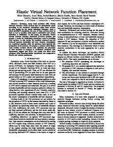
t3

t1

s3 m

s2

s1

t2 Fig. 1: Example: A minimum cardinality dominating set (three nodes, in light grey) is a bad approximation for the middlebox deployment problem (one node in center, in darker grey).

network nodes which can be dominated by a node is limited. Similarly, capacitated facility location problems [1], [5] ask for locations to deploy facilities, subject to capacity constraints, such that the number of facilities as well as the distance to the facilities are jointly optimized. In contrast to these problems where the distance to a dominator or facility from a given node is measured, in our middlebox deployment problem, we are interested in the distance (resp. stretch) between node pairs, via the middlebox. At first sight, one may intuitively expect that optimal solutions to dominating set or facility location problems are also good approximations for the middlebox deployment problem. However, this is not the case, as we illustrate in the following. Consider an optimal solution to the distance `/2 dominating set problem: since the distance to any dominator is at most `/2, the locations of the dominators are also feasible locations for the middleboxes: the route between two nodes via the dominator is at most `/2 + `/2 = `. However, the number of dominators in this solution can be much larger than the number of required middleboxes. Consider the example in Figure 1: in a star network where communicating node pairs are located at the leaves, at depth 1 and `−1, and where node capacities are sufficiently high such that they do not constitute a bottleneck, a single middlebox m in the center is sufficient. However, the stricter requirement that dominating nodes must be at distance at most `/2, results in a dominating set of cardinality Ω(n/`), i.e., Ω(n) for constant `. While our discussion revolved around constraints on the length `, similar arguments and bounds also apply to the stretch, the main focus of this paper: the ratio of the length of the path through a middlebox, and the length of the shortest path between the communicating pair. To see this, simply modify the example in Figure 1 by adding a direct edge between each communicating pair si and ti . Let c = `. Then the length of the shortest path between each pair is one. The dominating nodes must be at distance at most c/2 from the communicating nodes. Consequently, the cardinality of the dominating set is Ω(n/c), i.e., Ω(n) for constant c; deploying one single middlebox m at the center and routing the communication between each pair through m results in

3

t1 s4

s2

t3 m4

m2

m1

s1

g2

t2

t4

g1

m3

g3

s 3 f2

approach supports many alternative constraints, e.g., on the maximal route length. 3) Capacities are respected: at most κ node pairs can be served by any middlebox instance. Our objective is to minimize the number of required middlebox instances, subject to the above constraints. In this paper, we will also initiate the study of a weighted model, where different communication pairs have different demands, as well as a group model, where network functions need to serve entire groups of communication partners. See Figure 2 for an example. B. Use Cases

Fig. 2: Example: The communication between node pairs (si , ti ), for i ∈ {1, 2, 3, 4}, as well as between the group of nodes {g1 , g2 , g3 } needs to be routed via a network function resp. middlebox M . Due to capacity constraints and constraints on the route length, M is instantiated at four locations {m1 , m2 , m3 , m4 } in this example. paths of stretch c. D. Organization The remainder of this paper is organized as follows. Section II introduces our model and discusses different use cases. In Section III we present our approximation algorithm together with its analysis. Section IV extends our study to weighted and group models. After reporting on our simulation results in Section V, we conclude our contribution in Section VI. II. M ODEL AND U SE C ASES A. Formal Model We model the computer network as a graph connecting a set V of n = |V | nodes. The input to our problem is a set of communicating node pairs P : the route of each node pair (s, t) ∈ P needs to traverse an instance of a middlebox resp. network function (e.g., a firewall). Node pairs do not have to be disjoint: nodes can participate in many communications simultaneously. For the sake of generality, we assume that middleboxes can only be installed on a subset of nodes U ⊆ V . We will refer to the set of middleboxes locations (and equivalently, the set of middleboxes instances) by M , and we are interested in deploying a minimal number of middleboxes at legal locations M ⊆ U such that: 1) Each pair p = (s, t) ∈ P is assigned to an instance m ∈ M , denoted by m = µ(p). 2) For each pair p = (s, t) ∈ P , there is a route from s via m = µ(p) to t of length at most ρ · d(s, t), i.e., d(s, m) + d(m, t) ≤ ρ · d(s, t), where d(u, v) denotes the length of the shortest path between nodes u, v ∈ V in the network G, and where ρ ≥ 1 is called the stretch. For example, a stretch ρ = 1.2 implies that the distance (and the latency accordingly) when routing via a middlebox is at most 20% more than the distance (and the latency accordingly) when connecting directly. Our

Let us give three concrete examples motivating our formal model. Middlebox Deployment. Our model is mainly motivated by the middlebox placement flexibilities introduced in network function virtualized and software-defined networks. Deploying additional middleboxes, network processors or so-called “universal nodes” can be costly, and a good tradeoff should be found between deployment cost and routing efficiency. For example, today, network policies can often be defined in terms of adjacency matrices or big switch abstractions, specifying which traffic is allowed between an ingress port s and an outgress network port t. In order to enforce such a policy, traffic from s to t needs to traverse a middlebox instance inspecting and classifying the flows. The location of every middlebox can be optimized, but is subject to the constraint that the route from s to t via the middlebox should not be much longer than the shortest path from s to t. Deploying Hybrid Software-Defined Networks. There is a wide consensus that the transition of existing networks to SDN will not be instantaneous, and that SDN technology will be deployed incrementally, for cost reasons and to gain confidence. The incremental OpenFlow switch deployment problem can be solved using waypointing (routing flows via OpenFlow switches); our paper solves the algorithmic problem in the Panopticon [25] system. Distributed Cloud Computing. The first two use cases discussed above come with per-pair requirements: each communicating pair must traverse at least one function. However, there are also scenarios where entire groups Gi of nodes need to share a waypoint: for example, a multiplexer of a group communication (a multi-media conference) or a shared object in a distributed system, e.g., a shared and collaborative editor: An example could be a distributed cloud application: imagine a set of users Gi who would like to use a collaborative editor application a` la Google Docs. The application should be hosted on a server which is located close to the users, i.e., minimizing the latency between user pairs. III. A PPROXIMATION A LGORITHM A. Overview This section presents a deterministic and polynomial-time O(log(min{n, κ}))-approximation algorithm for the middlebox deployment problem. Our algorithm is based on an efficient computation of a certain submodular set function: it

4

defines the maximum number of pairs which can be covered by a given set of middleboxes. In a nutshell, the submodular function is computed efficiently using an augmenting path method on a certain bipartite graph, which also determines the corresponding assignment of communication pairs to the middleboxes. The augmenting path algorithm is based on a simple, linear-time breadth-first graph traversal. The augmenting path method is attractive and may be of independent interest: similarly to the flow-based approaches in the literature [6], it does not require changes to previously deployed middleboxes, but removes the disadvantage of [6] that the set of served communication pairs changes over time: an attractive property for incremental deployments. Our solution with augmenting paths results (theoretically and practically) in significantly faster computations of the submodular function value as well as of the corresponding assignment compared to the flow based approach. p In fact, computing all augmenting paths takes O(|E| min{ |V |, κ}) by using the p Hopcroft-Karp algorithm [21] performing at most O(min{ |V |, κ}) breadth-first search and depth-first search traversals of the graph. Computing a maximum flow takes O(|V ||E|2 ) time by the Edmonds-Karp algorithm [10], O(|V |3 ) time by the push-relabel algorithm of Goldberg and Tarjan [19], and O(|V ||E|) time by the algorithm of Orlin [31] (see [19] for an overview on efficient maximum flow algorithms). Concretely, we can start with an empty set of middlebox locations M = ∅, and in each step, we add a middlebox at location m to M , which maximizes the number of totally covered (by middleboxes at locations M ∪ {m}) communicating pairs, without violating capacity and route stretch constraints. The algorithm terminates, when all pairs were successfully assigned to middlebox instances in M . More precisely, for any set of middlebox instances M ⊆ U , we define φ(M ) to be the maximum number of communication pairs that can be assigned to M , given the capacity constraints at the nodes and the route stretch constraints. We show that φ is non-decreasing and submodular, and φ(M ) – and the corresponding assignment of pairs to middlebox instances in M – can be computed in polynomial time. This allows us to use Wolsey’s Theorem [40] to prove an approximation factor of 1+O(log φmax ), where φmax = maxm∈U φ({m}). Since in our case, φmax = min{κ, |P |} and |P | ≤ n2 , this implies that Algorithm 1 computes an O(log(min{κ, n}))-approximation for the minimum number of middlebox instances that can cover all pairs P (i.e., all pairs can be assigned to the deployed middleboxes). B. Maximum Assignment In order to compute function φ(M ), for any M ⊆ U , we construct a bipartite graph B(M ) = (M ∪ P, E), where P is the set of communicating pairs. We will simply refer to the middlebox instances m ∈ M and pairs p ∈ P in the bipartite graph as the nodes. The edge set E connects middlebox instances m ∈ M to those communicating pairs p ∈ P which can be routed via m without exceeding the stretch constraint, i.e. E = {(m, p) : m ∈ M, p = (s, t) ∈

Fig. 3: Bipartite graph with possible middlebox locations U (empty: white, deployed: grey) on the left side and pairs P on the right side of the bipartite graph. The capacity of the middleboxes κ = 2. Middleboxes are deployed greedily, oneby-one, without requiring relocation of previously mapped middleboxes. Assignment edges are indicated in bold. The deployment of the first middlebox left creates two assigment edges incident to the middlebox. The deployment of the second middlebox middle involves two new assigment edges incident to the second middlebox. Lastly, the botttom middlebox is used to serve the bottom pair, which was previously served by the middle middlebox.

P, d(s, m) + d(m, t) ≤ ρ · d(s, t)}, where d(u, v) denotes the length of shortest path between nodes u and v in the network. For each p, the set of such middlebox nodes can be computed in a pre-processing step by performing an allpair shortest paths algorithm to calculate d(u, v) for each u, v in the network, and for each p = (s, t) ∈ P , selecting the nodes m ∈ M with d(s, m) + d(m, t) ≤ ρ · d(s, t). A partial assignment A(M ) ⊆ B(M ) of pairs p ∈ P to middlebox instances in M is a subgraph of B(M ), in which each p ∈ P is connected to at most one middlebox m ∈ M by an edge, i.e., degA(M ) (p) ≤ 1 where deg denotes the degree. A pair p ∈ P with degA(M ) (p) = 1 is called an assigned pair and with degA(M ) (p) = 0 an unassigned pair of a free pair. A partial assignment A(M ) without free pairs is called an assignment. The size |A(M )| of a (partial) assignment A(M ) is defined as the number of edges in A(M ). Our goal is to compute a partial assignment A(M ) of pairs p ∈ P to middlebox instances in M maximizing the number of assigned pairs. Accordingly, we distinguish between assignment edges EA and non-assignment edges EA , where EA ∪EA = E is a partition of the edge set E of B(M ). Our algorithm ensures that at any moment of time, the partial assignments are feasible, i.e., the assignment fulfills the following capacity constraints. The current load of a middlebox m in M , denoted by λ(m), is the number of communicating pairs served by m according to the current partial assignment A(M ). Moreover, we define the free capacity κ∗ (m) of m to be κ∗ (m) = κ − λ(m). A (partial) assignment A(M ) is feasible if and only if it does not violate capacities, i.e., λ(v) ≤ κ, for all v in any middlebox in M . In order to compute the integer function φ(M ), which is essentially the cardinality of a maximum feasible partial assignment A∗ (M ), we make use of augmenting paths. Let A(M ) be a feasible partial assignment. An augmenting path

5

performing breadth-first searches in B(M ), by using the nodes m ∈ M with free capacities as the starting nodes. C. Submodularity

Fig. 4: Illustration of augmenting path computation. Bipartite graph with possible middlebox locations U (empty: white, deployed: grey) on the left side and pairs P on the right side of the bipartite graph. The capacity of the middleboxes κ = 2. Assignment edges are indicated in bold. Left: The assignment before deploying the third middlebox. Middle: Augmenting path starting at the new middlebox. Right: The resulting new assignment.

π = (v1 , v2 , . . . , vj ) relative to A(M ) in B(M ) starts at a middlebox m ∈ M with free capacity, ends at a free pair p ∈ P , and alternates between assignment edges and nonassignment edges, i.e., 1) v1 ∈ M with κ∗ (v1 ) > 0 and vj ∈ P with degA(M ) (vj ) = 0, 2) (vi , vi+1 ) ∈ B(M ) \ A(M ), for any odd i, 3) (vi , vi+1 ) ∈ A(M ), for any even i. An augmenting path relative to A(M ) is a witness for a better partial assignment: The symmetric difference A0 (M ) = (A(M ) \ π) ∪ (π \ A(M )) is also a (partial) assignment with size |A0 (M )| = |A(M )| + 1. Due to the properties of the augmenting path, by this reassignment, one additional pair will be covered by the same set of middlebox instances, without violating node capacities: in A(M ), the first node had free capacity and the last node represents a free pair. Furthermore, the degree at each internal node of π remains unchanged, since one incident assignment edge gets unassigned and one incident unassigned edge gets assigned. Therefore, the load of the internal nodes in π remains unchanged. Conversely, suppose that a partial assignment A(M ) is not a maximum partial assignment. Let A∗ (M ) be a maximum partial assignment. Consider the bipartite graph X = (A(M )∪A∗ (M ))\(A(M )∩ A∗ (M )). Figure 3 illustrates the greedy placement strategy and Figure 4 shows the augmenting path computation. Note that an augmenting path must always exist for suboptimal covers. To see this, consider the following reduction to matching: replace each middlebox node with κ many clones of capacity 1, and assign each pair p ∈ P to the clones in the canonical way. Feasible assignments constitute a matching in this graph, with node degrees one. Given any suboptimal cover, we find a witness for a augmenting path as follows. We take the symmetric difference of the suboptimal and the optimal solution, which gives us a set of paths and cycles of even length. Thus, a path must exist where the optimal solution has one additional edge. Augmenting paths can be computed efficiently, by simply

The set function φ : 2U → N is called non-decreasing iff φ(U1 ) ≤ φ(U2 ) for all U1 ⊆ U2 ∈ 2U , and submodular iff φ(U1 )+φ(U2 ) ≥ φ(U1 ∩U2 )+φ(U1 ∪U2 ) for all U1 , U2 ∈ 2U . Equivalently, submodularity can be defined as follows (See, e.g. in [37] pp. 766): for any U1 , U2 ⊆ U with U1 ⊆ U2 and every u ∈ U \ U2 , we have that φ(U1 ∪ {u}) − φ(U1 ) ≥ φ(U2 ∪ {u}) − φ(U2 ). This is in turn equivalent to: for every U1 ⊆ U and u1 , u2 ∈ U \ U1 we have that φ(U1 ∪ {u1 }) + φ(U1 ∪ {u2 }) ≥ φ(U1 ∪ {u1 , u2 }) + φ(U1 ). Let U1 ⊆ U2 be two arbitrary subsets of U . Consider a maximum assignment A(U1 ) for U1 . Let A(U2 ) be a maximum assignment for U2 obtained from A(U1 ) by adding the members u2 ∈ U2 \ U1 to U1 one-by-one, and performing the augmenting path method until we have a maximum assignment for the incremented set U1 ∪ {u2 }. Let AΠ (U1 ) be the projection of A(U2 ) to U1 , i.e., for each u1 ∈ U1 , p ∈ P , the pair p is assigned to u1 in AΠ (U1 ) if and only if p is assigned to u1 in A(U2 ). First we show that AΠ (U1 ) is a maximum assignment for U1 . Lemma 1. Let A(U1 ) be a maximum assignment for U1 . Let A(U2 ) be a maximum assignment for U2 obtained from A(U1 ) by adding all u ∈ U2 \ U1 to U1 one-by-one, and performing the augmenting path method until we have a maximum assignment for U1 ∪ {u}. Let AΠ (U1 ) be the projection of A(U2 ) to U1 . Then AΠ (U1 ) is a maximum assignment for U1 . Proof. By adding u2 ∈ U2 \ U1 to U1 and performing the augmenting path method until an augmenting path exists (i.e., until we obtain a maximum assignment for U1 ∪{u2 }), it holds that, for each u1 ∈ U1 , the number of pairs assigned to u1 does not change: along the augmenting path each internal node has one incident assignment edge and one non-assignment edge. This also holds after exchanging the assignment edges and the non-assignment edges, i.e., each assignment edge on the augmenting path becomes a non-assignment edge and vice versa. The degrees of the start and end nodes increases by one. Consequently, the degree of each u1 ∈ U1 in AΠ (U1 ) is the same as in A(U1 ). Since A(U1 ) is a maximum assignment and each u1 has the same degree in AΠ (U1 ), AΠ (U1 ) must be also a maximum assignment. Theorem 2. Let U be the set of all possible middlebox instance locations. Let φ : 2U → N be the set function, such that for M ⊆ U , φ(M ) is the maximum number of pairs in P that can be assigned to M without violating the capacity constraints. Then φ is submodular. Proof. We show that for all M1 , M2 ⊆ U , M1 ⊆ M2 and for all m ∈ U \ M2 we have that φ(M1 ∪ {m}) − φ(M1 ) ≥ φ(M2 ∪ {m}) − φ(M2 ).

(1)

This is equivalent to the definition of the submodularity of φ. Consider a maximum assignment A(M1 ) for M1 and a maximum assignment A(M2 ) for M2 obtained from A(M1 )

6

as described in Lemma 1. Now we add m to M2 . Let A(M2 ∪ {m}) be the maximum assignment for M2 ∪ {m} obtained from A(M2 ) by adding m to M2 and performing the augmenting path method until we have a maximum assignment for M2 ∪{m}. Let AΠ (M2 ) be the projection of A(M2 ∪{u}) to M2 and let AΠ (M1 ) be the projection of A(M2 ∪ {u}) to M1 . Let |AΠ (M2 )| and |AΠ (M1 )| be the number of assigned pairs of P in the assignments. By Lemma 1, AΠ (M2 ) is a maximum assignment for M2 and AΠ (M1 ) is a maximum assignment for M1 . Therefore, φ(M2 ) = |AΠ (M2 )| and φ(M1 ) = |AΠ (M1 )|. Furthermore, φ(M2 ∪ {u}) = |A(M2 ∪ {u})|. Consider the pairs Pm ⊆ P assigned to m in the assignment A(M2 ∪ {m}). Let AΠ (m) be the projection of A(M2 ∪ {m}) to m. Then |AΠ (m)| = |Pm |. Since AΠ (M2 ) contains all elements that are assigned to any element of M2 in A(M2 ∪ {m}), clearly |A(M2 ∪ {m})| = |AΠ (M2 )| + |AΠ (m)|, and thus φ(M2 ∪ {m}) − φ(M2 ) = |AΠ (m)|.

(2)

On the other side, the assignment A∗ (M1 ∪ {m}) which is obtained as the union of AΠ (M1 ) and AΠ (m) is a valid assignment for M1 ∪ {m}. Therefore, |A(M1 ∪ {m})| ≥ |A∗ (M1 ∪ {m})| = |AΠ (M1 )| + |AΠ (m)|, and thus φ(M1 ∪ {m}) − φ(M1 ) ≥ |AΠ (m)|.

(3)

Using (2) and (3) we obtain φ(M1 ∪ {m}) − φ(M1 ) ≥ φ(M2 ∪ {m}) − φ(M2 ) ,

(4)

completing our proof. D. The Algorithm Essentially, Algorithm 1 starts with an empty set M and cycles through the possible middlebox locations m ∈ U \ M , always deploying the middlebox resulting (with the already deployed ones) in the highest function value φ. Given the submodularity and the augmenting path construction, we have derived our main result. Per middlebox, an augmenting paths problem is solved. Using the HopcroftKarp algorithm, we can compute all (at most κ many) augmenting paths p starting at a newly added middlebox in time O(min{κ, |V |} · |E|), where |V | denotes the number of nodes and |E| the number of edges in B(M ). Theorem 3. Our greedy and incremental middlebox deployment algorithm computes a O(log n)-approximation. E. Lower Bound and Optimality Theorem 3 is essentially the best we can hope for: Theorem 4. The middlebox deployment problem is NP-hard and cannot be approximated within c log n, for some c > 0 unless P = N P . Furthermore, it is not approximable within (1 − ) ln n, for any  > 0, unless NP ⊂ D TIME(nlog log n ). Proof. We present a polynomial time reduction from the Minimum Set Cover (MSC) problem, defined as follows: Given a finite set S of n elements and a collection C of subsets

Algorithm 1: Greedy Algorithm 1: init M ← ∅, A(M ) ← empty assignment 2: while A(M ) is not a feasible assignment do 3: init m∗ ← ∅, opt ← 0, tmp ← 0 4: for each m ∈ U \ M (* compute all augmenting paths *) 5: tmp ← φ(M ∪ {m}) − φ(M ) 6: if tmp > opt then 7: opt ← tmp, m∗ ← m 8: end if 9: end for 10: M ← M ∪ {m∗ }, update A(M ) 11: end while

of S. A set cover for S is a subset C 0 ⊆ C such that every element in S is contained in at least one member of C 0 . The objective is to minimize the cardinality of the set cover C 0 . Consider an instance of the MSC problem: let S = {v1 , ..., vn } be a set of n elements, C = {Si ⊆ S, i = 1, ..., m}. We define the instance of the corresponding middlebox deployment problem in a network G = (V, E) with a set of communicating pairs P and stretch ρ = 1 as follows. For each element v ∈ S, we introduce two nodes vs and vt in V . For each subset Si ∈ C, we introduce a node vSi in V as well. The edge set E of the network G = (V, E) is defined by the following rule: there is an edge (vs , vSi ) ∈ E and an edge (vSi , vt ) ∈ E iff the corresponding element v is contained in Si . The set of communicating pairs is defined as P = {(vs , vt ) : v ∈ S} and the set of potential middlebox locations is defined as U = {vSi : Si ∈ C}. G = (V, E) is a bipartite graph with partitions U and {vs : v ∈ S} ∪ {vt : v ∈ S}. If v ∈ S is contained in a set Si ∈ C then there is a path of length 2 between the corresponding pair (vs , vt ) in G. This is also the shortest path between vs and vt . In the middlebox deployment problem with stretch ρ = 1, a set of nodes M ⊆ U of minimum cardinality must be selected such that between each pair (vs , vt ) ∈ P there is a route of length of at most 2 and it contains at least one node of M . By the construction of the network, for each pair (vs , vt ) ∈ P , there is a route vs , vSi , vt of length 2 in G if and only if v ∈ Si . Let M ⊆ U be a minimum cardinality solution of the middlebox deployment problem. The node set M implies a minimum cardinality solution for the MSC problem and vice versa. This proves the NP-hardness of the problem. The inapproximability results follow from the combination of the above reduction and the inapproximability results of the minimum set cover problem by Raz and Safra [35] and by Feige [15]. Raz and Safra [35] proved that the minimum set cover problem is not approximable within c log n, for some c > 0, unless P = N P . Feige [15] showed the inapproximability within (1 − ) ln n, for any  > 0, unless N P ⊂ D TIME(nlog log n ). If we had a better approximation for the middlebox deployment problem, by the above reduction, we would have a better approximation factor for the minimum set cover problem, as well.

7

Algorithm 2: Generalized Greedy Algorithm 1: init S ← ∅ 2: while |S| < |U | and f (S) ≤ n − 1 do 3: choose i ∈ U \ S s.t. gain(i, S) is maximized 4: S = S ∪ {i} 5: select middleboxes in set S 6: round f (S) to integer solution 7: end while

LP 1: Maximum Fractional Assignment X max f (S) = xi,j i,j

subject to

X

xi,j ≤ 1

∀j∈R

pj xi,j ≤ κ

∀i∈S

Xi∈U j∈R

xi,j = 0 0 ≤ xi,j ≤ 1

∀ i ∈ S, j ∈ R : pi,j > κ ∀ i ∈ S, j ∈ R

IV. G ROUP AND W EIGHTED VARIANT There are scenarios in which more than two nodes may have to share a network function. For example, consider the problem of placing a multiplexer for a group of users involved in a teleconference. Or imagine the problem of mapping a shared object or entire virtual server server of a multi-user game: in order to avoid state synchronization overheads, the users should be served from a single location which is also located close to all the users. Also in the context of distributed cloud computing, the problem of placing functionality for larger groups may be relevant. Moreover, so far we have assumed that all requests induce the same load. However, in reality, different communication pairs communicate at different rates, which may also result in different loads on the middleboxes. In this section, we show that both the group assignment variant as well as the weighted pair request variant can be solved by exploiting an interesting connection to energyefficient scheduling [16], [17], [23]. As we will see, in order to make this generalization, we will however need to sacrifice the incremental property. Moreover, we need a constant factor resource augmentation (concretely, a factor of 2). Let n be the total number of requests (set R), and let pj be the “price”, i.e., the load induced by assigning the j-th request to a middlebox: the request can be an arbitrarily weighted node pair or group of nodes. Our greedy algorithm runs in rounds, where in each round, the “most effective” middlebox, a middlebox at a location which maximizes a certain (submodular) function, is chosen and added to our solution set. Concretely, given a set S of already deployed middleboxes, let F (S) denote the maximum number of requests that can be processed by a set S of middleboxes of capacity κ. Since computing F (S) is NP-hard, we follow the work of [23] and compute a fractional solution using linear programming. The resulting fractional values will eventually be rounded. For every middlebox-request pair (i, j), we introduce a binary variable xi,j : it is 1, if request j is assigned to middlebox location i, and 0 otherwise. As a preprocessing step, let us first delete (1) all requests j with pj > κ, i.e., requests which cannot be served by any middlebox anyway; (2) all requestmiddlebox pairs which would exceed stretch constraints; and (3) all request-middlebox pairs where the middlebox is not at a legal location. We set the corresponding xi,j values to 0. We will relax the xi,j variables, and define f (S) to be the maximum weighted sum of requests that can be fractionally processed by a set S of middleboxes. We can compute f with Linear Program (LP) 1:

It follows from [16] that the relaxed function f is submodular. We define gain(i, S) = f (S ∪ {i}) − f (S) for any S ⊆ U , i ∈ U. The greedy algorithm (Algorithm 2) adds middleboxes one-by-one, greedily selecting the one yielding the highest gain(i, S). We stop when f (S) > n − 1: stopping prematurely is needed due to the fractional solution of the relaxed approach [23]. In the end, we round the fractional solution using the approach by Shmoys and Tardos [39]. Given this transformation, we can apply [23] and obtain that following approximation: with an augmentation factor of 2, we can serve all requests with at most a logarithmic factor more middleboxes. Theorem 5. The weighted resp. group network function placement problem can be (2, 1 + ln n)-approximated via the Generalized Greedy Algorithm in polynomial time, i.e., the number of deployed middleboxes is at most (1 + ln n) times the minimum and the maximum load on each middlebox is at most 2κ. Relationship to Datacenter Scheduling. Let us now elaborate more on the interesting relationship of this problem to datacenter scheduling problems. In the datacenter scheduling problem [23], we are given a set of m machines and n jobs. The processing time of job j on machine i is pi,j . Each machine i has an activation cost ai . The scheduling algorithm is given a total activation budget A, and needs to compute a subset of machines to activate which respect this budget constraint, and minimizes the makespan T : the length of the execution schedule. We translate this problem to our problem as follows. The machines correspond to the m possible middleboxes (set M corresponds to all possible locations U ), and the jobs correspond to the n requests. The cost of assigning a group resp. a weighted request j to a middlebox i corresponds to pi,j ; since in our model, this cost only depends on the request j but not on the middlebox i, we simply write pj instead of pi,j . The activation cost ai corresponds to the deployment cost and is the same for all middleboxes; we set ai = 1. In our algorithm, we greedily aim to select a subset of servers / middleboxes which maximize the (weighted sum of) covered requests. We need to cover all the requests, subject to middlebox capacity constraints κ, which correspond to the makespan.

8

V. E VALUATION In order to complement our formal analysis, we conduct a simulation study comparing the approximation algorithms presented above to the respective optimal algorithms implemented using Integer Programming (IP). We evaluate our greedy approximation algorithm using the following metrics: (1) the number of installed middleboxes and (2) runtime. Furthermore, we explore the performance of the approximation algorithm for the weighted variant and when incrementally deploying single middleboxes. All experiments were conducted on servers with two Intel XEON L5420 processors (8 cores overall) equipped with 16 GB RAM. A. Datasets We have generated two datasets, one for the unweighted approximation algorithm presented in Section III and one for the weighted approximation algorithm presented in Section IV. For the unweighted variant, we use real-world wide-area topologies obtained from the topology zoo collection [24]. As shown in Figure 5 (top), the topologies are either countrywide or continent-wide ISP, backbone, or – in case of Geant – research networks. The topologies were selected so that the number of nodes is equally spread across the range 20 to 82. Furthermore, the topologies provide detailed geographical information for nodes, such that communication latencies can be estimated based on the geographical distance. For each graph, we generate instances as follows: Each of the |V | · (|V | − 1)/2 potential communication pairs is selected with probability p, set to 0.2, 0.3, or 0.4, respectively. Hence, the number of expected communication pairs to be created overall is p · |V | · (|V | − 1)/2. To ensure comparability across topologies, all nodes are allowed to host middlebox functionality. The capacity κ is set to d2 · (|V | − 1) · pe: Hence, (in expectancy) around |V |/4 many middleboxes are likely to be necessary to serve the communication pairs. All communication pairs have the Name Quest GtsHungary Geant Surfnet Forthnet Telcove Ulaknet Name cost266 germany50 nobel-eu ta2

Type Continent Country Continent Country Country Country Country

Type Continent Country Continent Country

|V | 37 50 28 65

|V | 20 30 40 50 62 71 82 |E| 55 88 41 108

|E| 62 62 122 136 124 140 164 |D| 1,332 662 378 1,869

Fig. 5: Topology Zoo Instances (top) as well as SNDlib instances (bottom) used in the evaluation. |D| denotes the number of defined end-to-end communication requests.

same (latency) stretch. Concretely we set the maximal allowed latency to {1.00, 1.05, 1.10, . . . 2.50} times the latency of the shortest path between the nodes of the communication pair. For each topology and each probability, we generated 11 scenarios uniformly at random, yielding more than 7,000 instances overall. We employ a similar approach for the evaluation of the approximation algorithm for the weighted variant. Concretely, we consider four instances (see Figure 5 (bottom)) of the SNDlib [32], which already define communication pairs exhibiting a diverse demand structure. Analogously, we again consider stretches of {1.0, 1.05, . . . , 2.5}. To generate multiple instances from a single SNDlib instance, we sample requests by selecting each original communication pair independently at random with a probability of 0.5. We again allow to place middleboxes on all nodes in the network and set the capacity of each of the potential middlebox locations to 4 · D/|V |, where D denotes the cumulative demand of the chosen requests, such that at least 1/4 many nodes must be equipped with middleboxes. We generate 3,100 scenarios in total by considering 31 different stretch parameters and considering 25 random generated instances for the four different topologies. B. Baseline Algorithms Besides employing the approximation algorithms presented above, we use Integer Programs to compute optimal solutions. Integer Program (IP) 2 computes optimal solutions for the middlebox deployment problem with unitary demands1 and works as follows: For all potential middlebox locations u ∈ U , let Su be the set of pairs P that can be routed through u on a path of stretch at most ρ, i.e., Su = {p = (s, t) ∈ P : d(s, u) + d(u, t) ≤ ρ · d(s, t)}, where d(v, w) denotes the length of the shortest path between nodes v, w ∈ V in the network. Su can be precomputed efficiently. For all potential middlebox locations u ∈ U , we introduce the binary variable xu ∈ {0, 1}. The variable xu indicates that u is selected as a middlebox node in the optimal solution M , i.e. xu = 1 ⇔ u ∈ M . For all u ∈ U and p ∈ P , we introduce the binary variable xup ∈ {0, 1}. The variable xup indicates that the pair p = (s, t) ∈ P is assigned to the node u ∈ U , s.t. the path stretch from s to t through u is at most ρ. The Objective Function (5) requires that a minimum cardinality middlebox set must be selected. Constraints (6) declare that each pair p = (s, t) ∈ P is assigned to exactly one node u ∈ U . Constraints (7) state that each pair p = (s, t) ∈ P can only be assigned to a node u ∈ U with p ∈ Su . By the definition of Su , the pair p can be routed through u via a path of stretch at most ρ. Constraints (8) describe that the capacity limit κ must not be exceeded at any node, and nodes u ∈ U which are not selected in the solution M (where the corresponding variable xu becomes 0 in the solution) are not assigned to any pair p ∈ P . This Integer Program can easily be adapted for the weighted (and or group) variant by adapting Constraint (8). Concretely, 1 The existence of a 0-1 integer linear program, together with our NPhardness result, also proves the NP-completeness [22].

9

∀p∈P

(11)

xu = n

∀p∈P

(12)

of 31 × 11 = 341 experiments. The average runtime of the sequential greedy-algorithm lies below the one of the IP for 20 and 30 nodes, and the greedy algorithm with 8 threads clearly outperforms the IP on the topologies with 62, 71 and 82 nodes. On the largest topology the computation of the greedy algorithm can be sped up by a factor of around 5, by using 8 threads. Furthermore, the runtime of the IP is on the largest topology one magnitude higher than the one of the 8-threaded greedy algorithm. The left plot of Figure 6 depicts the runtime of the 8-threaded greedy variant and the IP on the largest topology as a function of the stretch. Starting at a stretch of 1.3, the runtime of the IP increases dramatically. This is due to the fact that by increasing the stretch, the number of potential middleboxes, serving a communication pair, increases. In fact, on the largest topology, the IP consisted of up to 90k variables. Regarding the number of installed middleboxes, the left box plot of Figure 6 shows the approximation ratio, i.e., the number of middleboxes opened by the greedy algorithm divided by the optimal number of middleboxes computed by the IP. The median lies below 1.5 and the maximum is close to 1.8.

u∈U X xup = 0

∀u∈U

(13)

D. Weighted Requests

∀u∈U

(14)

IP 2: Baseline for Minimizing the Number of Middleboxes X min xu (5) u∈U

subject to

X

xup = 1

∀p∈P

(6)

xup = 0

∀u∈U

(7)

xup ≤ κ · xu

∀u∈U

(8)

∀ u ∈ U, p ∈ P

(9)

u∈U

X p6∈Su

X p∈P

xu , xup ∈ {0, 1}

IP 3: Maximum Assignment for exactly n Middleboxes X max xup (10) u∈U

subject to

X

xup ≤ 1

u∈U

X

p6∈Su

X

xup ≤ κ · xu

p∈P

xu , xup ∈ {0, 1}

∀ u ∈ U, p ∈ P (15)

Constraint 8 needs to include the additional factor dp , denoting the demand of request p: X dp · xup ≤ κ · xu ∀u ∈ U . p∈P

As we are also interested in studying the opportunities arising in incremental deployment scenarios, we also introduce IP 3 which computes the maximum assignment for any given number of middleboxes. Concretely, given a number n ∈ N of middleboxes to activate (see Constraint 12), the number of connected communication pairs is maximized (see Constraint 10), while ensuring that a communication pair may at most be assigned to exactly one middlebox (see Constraint 11). We have implemented the IPs in Python using Gurobi 6.5. C. Runtime and Number of Middleboxes We first study the runtime and the empirical approximation factor of the approximation algorithm 1 on the randomly generated topology zoo instances. To this end, we have implemented the greedy approximation algorithm in Python. Our implementation may use multi-threading for the computation of the middlebox-selection in Algorithm 1 (Lines 4-9). The computation of the Integer Program solutions is implemented via Gurobi 6.5 using a single thread. In Figure 6 (right and bottom), the average runtime of the greedy (G) approximation algorithm with 1 and 8 threads, and the IP is depicted. In the middle plot the averaged runtimes are shown. Here, each data point represents the aggregate

Next, we study the performance of the approximation algorithm discussed in Section IV, for weighted problems (cf. Algorithm 2). As discussed in Section V-A, we use SNDlib instances exhibiting a diverse demand structure (see Figure 7 left). Again, we have implemented the generalized approximation algorithm and the corresponding adaption of Integer Program 2 in Python. As a first result, the middle plot of Figure 7 shows the averaged relative number of deployed middleboxes of the greedy algorithm with respect to the optimal solution of the IP. The greedy approximation algorithm only seldomly opens – on average – more than 20% middleboxes more than the optimal algorithm. Note that, in some cases, the number of deployed middleboxes lies even beneath the optimal one. This is possible, as the considered algorithm may (cf. Figure 7 right) violate the middlebox capacity up to a factor of 2. Indeed, the approximation algorithm violates capacities in less than 25% of the cases (cf. Figure 7). E. Incremental Middlebox Activation Lastly, we study scenarios in which middleboxes are added one after another. Concretely, we assume that all communication pairs are known in advance while the network operator can only incrementally install single middleboxes (e.g. due to the associated cost). The greedy algorithm always places one additional middlebox while not being allowed to change previously selected middlebox locations. We study the number of assigned communication pairs of the greedy algorithm compared to the optimum number of assignments when middlebox locations may be arbitrarily selected. To compute the optimum number of assignments the IP 3 is used. We consider the same experimental setup as described in Section V-C (i.e. topology zoo instances), while constraining the probability to create communication pairs to p = 0.3.

102

20 30 40 50 62 71 82 number of nodes

101

1000

p=0.2 p=0.3 p=0.4 G(1) G(8) IP

100 10-1

p=0.2 p=0.3 p=0.4 G(8) IP

800 runtime (s)

1.8 1.7 1.6 1.5 1.4 1.3 1.2 1.1 1.0

runtime (s)

approximation ratio

10

600 400 200 0

20 30 40 50 60 70 80 number of nodes

1.0 1.2 1.4 1.6 1.8 2.0 2.2 2.4 stretch

Fig. 6: Left: Empirical approximation ratio. Middle: Runtime of the algorithms as a function of the different topologies. Right: Runtime as a function of the stretch on the Ulaknet topology.

ECDF

0.8 0.6

Demand Distribution cost266 germany50 nobel-eu ta2

0.4 0.2 0.0 -4 10

10 -3

10 -2

10 -1

relative demand size

10 0

Greedy Loads

1.25 Relative number of Opened Middleboxes 1.20 1.15 1.10 1.05 1.00 cost266 0.95 germany50 0.90 nobel-eu 0.85 ta2 0.80 1.0 1.2 1.4 1.6 1.8 2.0 2.2 2.4 2.6 stretch

2.0 relative load

1.0

1.5 1.0 0.5 0.0 1.0

1.25

1.5

1.75 2.0 stretch

2.25

2.5

Fig. 7: Left: The demand structure on the SNDlib instances as empirical cumulative distribution function. Middle: The relative number of opened middleboxes compared to the solution of the baseline IP. Right: The relative load, i.e. load divided by the available capacity, on the middleboxes computed by the (2, 1 + ln n)-approximation algorithm.

VI. S UMMARY AND C ONCLUSION This paper initiated the study of the network function placement problem which is motivated by the increasing flexibilities of modern virtualized networked systems. Our main

5 10 15 20 25 5

10

15

20

25

greedily placed

30

0.14 0.12 0.10 0.08 0.06 0.04 0.02 0.00

Optimal Number of Middleboxes

600

absolute frequency

Relative Difference of Assignments optimally placed

We present the results of this set of experiments in Figure 8. The left plot depicts the relative difference of assigned communication pairs when using the greedy algorithm compared to the IP baseline. Concretely, the relative difference is defined as (φIP − φG )/φIP , where φIP and φG denotes the number of assigned communication pairs of the IP and the greedy algorithm, respectively. The rows of the left plot averages the results for all scenarios having the same number of minimal middleboxes to serve all communication pairs. The number of scenarios averaged in this way is depicted in the right plot of Figure 8: the number of scenarios for which 10 middleboxes suffice and which are averaged in the row 10 is for example around 520. Considering any row, we see that the greedy algorithm assigns nearly always as many communication pairs until the number of middleboxes reaches the optimum (minimal) number of middleboxes. After coming close to the optimum number of middleboxes, the relative difference in assignments reaches a maximum valiue of 0.15 and then diminishes only slightly with each additional greedily placed middlebox. The ability to (re-)place middleboxes in an arbitrary fashion hence only becomes important when sufficiently many middleboxes were already places to serve almost all communication pairs.

500 400 300 200 100 0

0

5

10

15

20

placed middleboxes

25

30

Fig. 8: Left: The averaged relative difference in the number of served communications pairs depending on the optimal number of middleboxes (y-axis). Right: Minimum number of middleboxes computed by the IP for the scenarios averages in the left plot.

contribution is a combinatorial proof of the submodularity of this problem and an incremental log-approximation network function placement algorithm. We also initate the study of a randomized rounding approach for a weighted group-version of the problem. Our simulation results show that this approach computes a nearly optimal placement for real world network instances. We understand our work as a first step, and believe that our paper opens several interesting directions for future research. In particular, it will be interesting to know whether good approximations exist for the incremental deployment of entire group requests.

11

R EFERENCES [1] K. Aardal, P. L. van den Berg, D. Gijswijt, and S. Li. Approximation algorithms for hard capacitated k-facility location problems. European Journal of Operational Research, 242(2):358–368, 2015. [2] A. Abujoda and P. Papadimitriou. MIDAS: middlebox discovery and selection for on-path flow processing. In Proc. 7th COMSNETS, pages 1–8, 2015. [3] M. Bagaa, T. Taleb, and A. Ksentini. Service-aware network function placement for efficient traffic handling in carrier cloud. In Proc. IEEE Wireless Communications and Networking Conference (WCNC), pages 2402–2407, 2014. [4] N. Bansal, R. Krishnaswamy, and B. Saha. On capacitated set cover problems. In Approximation, Randomization, and Combinatorial Optimization. Algorithms and Techniques - 14th International Workshop, APPROX 2011, and 15th International Workshop, RANDOM 2011, Proceedings, pages 38–49, 2011. [5] F. A. Chudak and D. P. Williamson. Improved approximation algorithms for capacitated facility location problems. Mathematical Programming, 102(2):207–222, 2005. [6] J. Chuzhoy and J. Naor. Covering problems with hard capacities. In Proc. IEEE FOCS, pages 481–489, 2002. [7] J. Chuzhoy and J. Naor. Covering problems with hard capacities. SIAM J. Comput., 36(2):498–515, 2006. [8] V. Chvatal. A greedy heuristic for the set-covering problem. Mathematics of Operations Research, 4(3):233–235, 1979. [9] D. Levin et al. Panopticon: Reaping the benefits of incremental sdn deployment in enterprise network. In Proc. USENIX ATC, 2014. [10] J. Edmonds and R. M. Karp. Theoretical improvements in algorithmic efficiency for network flow problems. J. ACM, 19(2):248–264, 1972. [11] G. Even, M. Medina, and B. Patt-Shamir. Online path computation and function placement in sdns. In Proc. 18th International Symposium on Stabilization, Safety, and Security of Distributed Systems (SSS), 2016. [12] G. Even, M. Rost, and S. Schmid. An approximation algorithm for path computation and function placement in sdns. In Proc. 23rd International Colloquium on Structural Information and Communication Complexity (SIROCCO), 2016. [13] S. Fayazbakhsh et al. Flowtags: Enforcing network-wide policies in the presence of dynamic middlebox actions. In Proc. ACM HotSDN, 2013. [14] N. Feamster, J. Rexford, and E. Zegura. The road to SDN. Queue, 11(12), 2013. [15] U. Feige. A threshold of ln n for approximating set cover. J. ACM, 45(4):634–652, 1998. [16] L. Fleischer. Data center scheduling, generalized flows, and submodularity. In Proc. 7th Workshop on Analytic Algorithmics and Combinatorics, (ANALCO), pages 56–65, 2010. [17] M. Gairing, B. Monien, and A. Woclaw. A faster combinatorial approximation algorithm for scheduling unrelated parallel machines. Theoretical Computer Science, 380(1-2):87–99, 2007. [18] A. Gember-Jacobson et al. OpenNF: Enabling innovation in network function control. In Proc. ACM SIGCOMM, pages 163–174, 2014. [19] A. V. Goldberg and R. E. Tarjan. A new approach to the maximum-flow problem. J. ACM, 35(4):921–940, 1988. [20] R. Hartert, P. Schaus, S. Vissicchio, and O. Bonaventure. Solving segment routing problems with hybrid constraint programming techniques. In Proc. International Conference on Principles and Practice of Constraint Programming (CP), 2015. [21] J. E. Hopcroft and R. M. Karp. An n5/2 algorithm for maximum matchings in bipartite graphs. SIAM Journal on Computing, 2(4):225– 231, 1973. [22] R. M. Karp. Reducibility among combinatorial problems. In Complexity of Computer Computations, pages 85–103. 1972. [23] S. Khuller, J. Li, and B. Saha. Energy efficient scheduling via partial shutdown. In Proc. ACM-SIAM Symposium on Discrete Algorithms (SODA), pages 1360–1372, 2010. [24] S. Knight, H. Nguyen, N. Falkner, R. Bowden, and M. Roughan. The internet topology zoo. Selected Areas in Communications, IEEE Journal on, 29(9):1765 –1775, october 2011. [25] D. Levin, M. Canini, S. Schmid, F. Schaffert, and A. Feldmann. Panopticon: Reaping the benefits of incremental sdn deployment in enterprise networks. In Proc. USENIX Annual Technical Conference (ATC), pages 333–345, 2014. [26] T. Lukovszki, M. Rost, and S. Schmid. It’s a match! near-optimal and incremental middlebox deployment. ACM SIGCOMM Computer Communication Review (CCR), 46(1):30–36, 2016.

[27] T. Lukovszki and S. Schmid. Online admission control and embedding of service chains. In Proc. 22nd International Colloquium on Structural Information and Communication Complexity (SIROCCO), pages 104– 118, 2015. [28] C. Lund and M. Yannakakis. On the hardness of approximating minimization problems. J. ACM, 41(5):960–981, 1994. [29] M. Markovitch and S. Schmid. Shear: A highly available and flexible network architecture: Marrying distributed and logically centralized control planes. In Proc. 23rd IEEE International Conference on Network Protocols (ICNP), 2015. [30] S. Mehraghdam, M. Keller, and H. Karl. Specifying and placing chains of virtual network functions. In Proc. IEEE CloudNet, pages 7–13, 2014. [31] J. B. Orlin. Max flows in O(nm) time, or better. In Proc. ACM STOC, pages 765–774, 2013. [32] S. Orlowski, M. Pi´oro, A. Tomaszewski, and R. Wess¨aly. Sndlib 1.0 – Survivable Network Design Library. Networks, 55(3):276–286, 2010. [33] Z. Qazi et al. SIMPLE-fying middlebox policy enforcement using SDN. In Proc. ACM SIGCOMM, pages 27–38, 2013. [34] W. Rankothge, J. Ma, F. Le, A. Russo, and J. Lobo. Towards making network function virtualization a cloud computing service. In Proc. IFIP/IEEE International Symposium on Integrated Network Management (IM), pages 89–97, 2015. [35] R. Raz and S. Safra. A sub-constant error-probability low-degree test, and sub-constant error-probability PCP characterization of NP. In Proc. ACM STOC, pages 475–484, 1997. [36] S. Raza, G. Huang, C.-N. Chuah, S. Seetharaman, and J. P. Singh. Measurouting: A framework for routing assisted traffic monitoring. IEEE/ACM Trans. Netw., 20(1):45–56, 2012. [37] A. Schrijver. Combinatorial Optimization – Polyhedra and Efficiency. Springer-Verlag, 2003. [38] J. Sherry et al. Making middleboxes someone else’s problem: Network processing as a cloud service. In Proc. ACM SIGCOMM, pages 13–24, 2012. [39] D. B. Shmoys and E. Tardos. An approximation algorithm for the generalized assignment problem. Math. Program., 62(3):461–474, Dec. 1993. [40] L. Wolsey. An analysis of the greedy algorithm for the submodular set covering problem. Combinatorica, 2(4):385–393, 1982.