sphere and the associated orientations on this design sphere which are nearest the n ... niques. It is essential that the spherical mechanism designer be.
David M. Tse Pierre M. Larochelle* Robotics and Spatial Systems Laboratory, Mechanical Engineering Program, Florida Institute of Technology, Melbourne, FL 32901
Approximating Spatial Locations With Spherical Orientations for Spherical Mechanism Design In this paper we present a novel method for approximating a finite set of n spatial locations1 with n spherical orientations. This is accomplished by determining a design sphere and the associated orientations on this design sphere which are nearest the n spatial locations. The design sphere and the orientations on it are optimized such that the sum of the distances between each spatial location and its approximating spherical orientation is minimized. The result is a design sphere and n spherical orientations which best approximate a set of n spatial locations. In addition, we include a modification to the method which enables the designer to require that one of the n desired spatial locations be exactly preserved. This method for approximating spatial locations with spherical orientations is directly applicable to the synthesis of spherical mechanisms for motion generation. Here we demonstrate the utility of the method for motion generation task specification in spherical mechanism design. 关S1050-0472共00兲00204-X兴
Introduction Spherical mechanisms are linkages which generate spherical motion of rigid bodies. In spherical motion, the displacement of any point on the body is constrained to the surface of a sphere. In contrast, planar mechanisms generate two-dimensional motion. For this reason their design is compatible with using conventional drafting tools while the synthesis of spherical mechanisms is three-dimensional and is not well suited for these drafting techniques. It is essential that the spherical mechanism designer be able to visualize the entire problem in three-dimensions and computer graphics can be an effective tool for providing this necessary visualization of the problem to the designer. Efforts have been made to create computer graphics based software packages for spherical four-bar mechanism design: • SPHINX was the first spherical mechanism computer-aided design 共CAD兲 program written by Larochelle et al. 关1兴 for use on Silicon Graphics workstations. SPHINX begins by displaying a design sphere. The design sphere defines the surface in space upon which the workpiece is to be moved. The relative displacements between the locations on the design sphere are purely rotational and are called orientations. Orientations are defined by their longitude, latitude, and roll angles 关2兴. In SPHINX orientations are displayed to the designer as coordinate frames on the surface of the design sphere, see Fig. 1. The current version of SPHINX has modules for performing synthesis for three or four orientation rigid body guidance. It is important to note that in SPHINX the design sphere is of arbitrary radius and its location in space is undefined. • SPHINXPC 关3兴 is a CAD program for personal computers which like SPHINX utilizes a design sphere with orientations displayed on the sphere’s surface. With this software spherical mechanisms can be designed for four orientations. SPHINXPC also can be used to design planar mechanisms for four location rigid body guidance. • SPHEREVR 关4兴 is the first virtual reality 共VR兲 based approach
to spherical mechanism design. This initial exploration of the use of VR for spherical mechanism design has led to the development of a 3rd generation of VR based spherical mechanism design software called ISIS, see Larochelle, Vance, and McCarthy 关5兴. The program utilizes the compute engine of SPHINX1.2 and provides virtual objects in the design environment so that the design process takes place in a virtual representation of the physical workspace. This new approach to mechanism design has demonstrated a need for new and efficient means for specifying the design task in the actual physical workspace of the mechanism. To synthesize a spherical mechanism, the designer must first define the task to be accomplished. Here we are concerned with task specification for moving a workpiece through a sequence of prescribed orientations in space. This task is referred to as rigidbody guidance by Suh and Radcliffe 关6兴 and as motion generation by Erdman and Sandor 关7兴. An example of a rigid body guidance task is shown in Fig. 2. The desired locations of the workpiece are defined in space. A coordinate frame is attached to the workpiece and each of its desired locations is recorded. To date, when designing spherical mechanisms the designer must determine an appropriate design sphere, i.e. its center and radius, from the desired
*Address all correspondence to this author. 1 The location or pose of a rigid body is defined by both its orientation and position; the position is defined by three coordinates which uniquely define where a point of the body is and the orientation is defined by three angles which orient the body with respect to a fixed reference body. Contributed by the Mechanisms Committee for publication in the JOURNAL OF MECHANICAL DESIGN. Manuscript received July 1998. Associate Technical Editor: C. M. Gosselin.
Journal of Mechanical Design
Copyright © 2000 by ASME
Fig. 1 SPHINX DESIGN SPHERE
DECEMBER 2000, Vol. 122 Õ 457
q 1 ⫽s x sin ⫽s x s 2 2 q 2 ⫽s y sin ⫽s y s 2 2
(1)
q 3 ⫽s z sin ⫽s z s 2 2 q 4 ⫽cos ⫽c 2 2 where s and are the rotation axis and the angle of rotation associated with the orientation, respectively. Note that the components of q satisfy the following constraint equation, q 21 ⫹q 22 ⫹q 23 ⫹q 24 ⫺1⫽0
Fig. 2 A desired task
spatial locations. Moreover, the sets of angles which define the orientations of the body with respect to that design sphere must also be determined. Currently, no methodologies exist to facilitate this process. It is only after determining the design sphere and the orientations that the designer can utilize CAD tools such as SPHINX and SPHINXPC. In this paper, one method of determining the optimal design sphere and orientations from a desired set of spatial locations is presented. First, the spatial locations are approximated with orientations in four-dimensional Euclidean space (E4 ). Biquaternions are then used to represent these orientations. Next, the distance between the spatial locations and the orientations on a candidate design sphere are calculated using a bi-invariant metric on biquaternions. Finally, an optimization method is used to minimize the distances between the spherical orientations on the candidate design sphere and the spatial locations. The result is a procedure which numerically determines the optimal design sphere and orientations for a finite set of desired spatial locations.
and lie on a unit hypersphere which we denote as the image space of spherical displacements, see Larochelle 关10兴 and McCarthy 关11兴. Recall that the location of a body in E3 has six degrees of freedom 共three to define orientation and three to define location兲 and can be represented by a 4⫻4 homogeneous transform 关12兴:
T⫽
⯗
d
........................ 0
0
0
⯗
1
册
(3)
where d is a 3⫻1 translation vector. The angles , , and are the longitude, latitude, and roll angles respectively 关2兴. In 1996 Etzel and McCarthy 关8兴 showed that a 4⫻4 homogeneous transform in E3 can be approximated by a pure rotation in E4 , 关 D 兴 ⫽ 关 J 共 ␣ ,  , ␥ 兲兴关 K 共 , , 兲兴
where,
J 共 ␣ ,  , ␥ 兲 ]⫽
Orientations in E and Biquaternions
458 Õ Vol. 122, DECEMBER 2000
冋
关 R 共 , , 兲兴
关 R 共 , , 兲兴 ⫽Roty 共 兲 Rotx 共 ⫺ 兲 Rotz 共 兲
4
In 关2兴 Larochelle and McCarthy presented an algorithm for approximating a set of n locations in planar Euclidean space (E2 ) with n spherical orientations in three-dimensional Euclidean space (E3 ). By utilizing a bi-invariant metric on the image space of spherical displacements they arrived at an approximate biinvariant metric for planar locations in which the error induced by the spherical approximation is of the order 1/R2 , where R is the radius of the approximating sphere. In this paper we extend their methodology to the general spatial case and utilize the results to provide a novel method of specifying motion generation tasks for spherical mechanisms. It was shown in Larochelle and McCarthy 关2兴 that orientations in E3 may be used to approximate locations in a bounded region of a two-dimensional plane. We utilize the contributions of Etzel and McCarthy 关8兴 and extend that idea by using orientations in E4 to approximate locations in a bounded region of three-dimensional space. This can be done by using a small portion of a fourdimensional hypersphere, a wedge, to approximate a bounded region of space. Orientations on the surface of this wedge, which we represent with biquaternions, can be used to approximate the spatial locations. See Ge 关9兴 in which he examines the theory of biquaternions as representations of orientations on a hypersphere. We proceed by briefly reviewing quaternions and biquaternions. Recall that an orientation in E3 can be represented by a quaternion q⫽ 关 q 1 q 2 q 3 q 4 兴 T . The four components of the quaternion q 共sometimes referred to as Euler parameters兲 are,
(2)
冋
(4)
c␣
0
0
s␣
⫺s  s ␣
c
0
sc␣
⫺s ␥ c  s ␣
⫺s ␥ s 
c␥
s␥cc␣
⫺c ␥ c  s ␣
⫺s  c ␥
⫺s ␥
c␥cc␣
and,
K 共 , , 兲 ]⫽
冋
关 R 共 , , 兲兴
⯗
0
⯗
0
⯗
0
........................ 0
0
0
⯗
1
册
册
.
The angles ␣,  and ␥ are defined as follows: tan(␣)⫽dx /R, tan()⫽dy /R, and tan(␥)⫽dz /R where d x , d y , and d z are the components of d and R is the radius of the hypersphere. The bounded spatial workspace must represent only a small portion of the hypersphere 共i.e. a wedge兲, hence we determine the radius of the hypersphere as: R⫽
4L ⑀ 1/2
(5)
where L is the largest component of the translation vectors from the set of spatial locations and ⑀ is the maximum allowable error in the approximation of the spatial locations with the orientations in E4 . The result is that the n spatial locations lie within a 2L cube and the wedge approximates a 4L cube, with the center of each cube being the origin of E3 . It is important to note that the selection of R determines the metric’s weighting between rotational Transactions of the ASME
distance and translational distance. As R→⬁ the metric disregards translational distances and as R→0 the metric disregards rotational distances, see Larochelle 关13兴. The radius selection formula used here was shown by Larochelle 关13兴 to yield a metric which incorporates both the translation distance and the rotation distance between two spatial locations but the rotation is more heavily weighted. This is appropriate since we are seeking to design spherical mechanisms to accomplish spatial tasks. Next, we review how to determine the biquaternion associated with the matrix 关 D 兴 . Recall that biquaternions have the following form: ˆ ⫽G⫹ H G
(6)
where G and H are quaternions and is defined such that 2 ⫽1, see Ge 关9兴. The biquaternion can also be represented as an ˆ ⫽(G,H). The quaternions G and H ordered pair of quaternions G are determined by the following computations. The fourth components of G and H are G 4 ⫽cos() and H 4 ⫽cos() respectively, with and being the real part of the eigenvalues from matrix 关 D 兴 . The other three components of G and H are computed as follows: G 1⫽
d 23⫺d 32⫹d 14⫺d 41 4H 4
冉
d 31⫺d 13⫹d 42⫺d 24 G 2 ⫽⫺ 4H 4 G 3⫽
d 21⫺d 12⫹d 34⫺d 43 4H 4
H 1⫽
d 32⫺d 23⫺d 14⫹d 41 4G 4
冉
d 31⫺d 13⫺d 42⫹d 24 H 2 ⫽⫺ 4G 4 H 3⫽
冊 冊
where d i j are the elements of 关 D 兴 . From the above relations, it is evident that there are three special cases which need to be addressed, see Etzel 关14兴. First, if G 4 ⫽0 then the first three elements of H are: d 11⫹d 44 H 1⫽ 2G 1
H 3⫽
d 22⫽d 44 2G 2
d 33⫹d 44 . 2G 3
Second, if H 4 ⫽0 then the first three components of G are: d 11⫹d 44 G 1⫽ 2H 1 G 2⫽ G 3⫽
ˆ ,R ˆ 兲 ⫽ 冑共 Q⫺R兲 T共 Q⫺R兲 ⫹ 共 S⫺T兲 T共 S⫺T兲 d共 Q
(7)
ˆ ⫽(Q,S) and R ˆ ⫽(R,T) are both biquaternions. For a where Q proof that this metric is bi-invariant see Etzel and McCarthy 关8兴.
Optimizing the Design Sphere
d 21⫺d 12⫺d 34⫹d 43 4G 4
H 2⫽
defining similar useful metrics for determining the distance between two locations of a rigid body is still an area of ongoing research, see Kazerounian and Rastegar 关15兴, Bobrow and Park 关16兴, Martinez and Duffy 关17兴, Larochelle and McCarthy 关2兴, Etzel and McCarthy 关8兴, and Gupta 关18兴. In the case of two locations of a rigid body in E3 any metric used to measure the distance between the locations yields a result which depends upon the chosen reference frames, see Martinez and Duffy 关17兴. However, Ravani and Roth 关19兴 define the distance between two orientations in E3 as the magnitude of the difference between their associated quaternions, which is a bi-invariant metric2. Etzel and McCarthy 关8兴 extended this idea and presented a bi-invariant metric for orientations in E4 . Here, we review their metric and present a methodology which employs the metric to determine the optimal design sphere associated with a finite set of spatial locations. The bi-invariant metric on biquaternions is defined as:
In Fig. 3 a spherical orientation on a design sphere is shown. To obtain the orientation frame relative to the fixed frame three coordinate frame transformations are applied. First, the moving frame is translated along the 3⫻1 center vector c. Next, the moving frame is rotated by the longitude, latitude, and roll angles as defined by Eq. 3. Third, the moving frame is translated along the 3⫻1 radial vector r. The spherical orientation is now defined by the following 4⫻4 homogeneous transform:
冋
]
关R兴
关 R 兴 r⫹c
T spherical共 r,c兲 ⫽ .............................. 0
0
0
]
1
册
where 关 R 兴 is the 3⫻3 rotation matrix defined in Eq. 3. Let T spatial be the 4⫻4 homogeneous transform representation of a desired location of the workpiece in space, see Eq. 3. To determine the optimal design sphere the distance between T spatial and T spherical must be minimized for each of the n desired locations in E3 . The next section presents a method to minimize this distance by utilizing the bi-invariant metric discussed above. Optimization. Given a finite set of n desired locations in E3 the task is to determine the optimal design sphere and the n orientations on that sphere. By examining the homogeneous transform representation of T spherical it is clear that the optimization variables are r and c since 关 R 兴 may be extracted from T spatial3. The optimization problem then becomes: 2 Recall that a bi-invariant metric is independent of choice of both the fixed and moving frames. 3 Note that by extracting 关 R 兴 in this manner we guarantee that the orientations of the nT spherical will be identical to that of their associated T spatial .
d 22⫹d 44 2H 2
d 33⫹d 44 . 2H 3
Finally, if G 4 ⫽0 and H 4 ⫽0 then solve the following relations for H i (i⫽1,2,3): d 21⫺d 43 d 11⫹d 44 d 31⫹d 42 ⫽ ⫽ H2 H1 H3 and obtain G i as in the H 4 ⫽0 case above. The Metric. There exist numerous useful metrics for defining the distance between two points in Euclidean space, however, Journal of Mechanical Design
Fig. 3 Optimal design sphere
DECEMBER 2000, Vol. 122 Õ 459
The initialization of r is obtained by equating the translation vectors of T spatial and T spherical . For any given spatial location the radial vector r of the design sphere is then, r⫽ 关 R 兴 T 共 dspatial⫺c兲 .
(9)
Substituting cinitial into Eq. 9 we obtain: r⫽ 关 R 兴 T 共 dspatial⫺cinitial兲 .
(10)
Using Eq. 10 we compute r for each spatial location. The initial estimation of the radial vector is then the average, n
rinitial⫽
冋
Minimize:
Subject to:
]
关 R exact兴
dexact
0
0
⯗
0
1
册
n
兺 d 共 Qˆ ,Rˆ 兲 i
i
ˆ i and Rˆ i are the biquaternion representations of the n and Q T spherical and T spatial respectively. Note that the magnitudes of both r and c are bounded to insure that the design sphere remains within the 4L cube of E3 that is being approximated by the hypersphere’s wedge, see Eq. 5. We utilize the simplex method for function minimization to find r and c that minimize f (r,c), see Nelder and Mead 关20兴. This method was selected since it does not require analytical gradients and it is a direct multidimensional minimization algorithm. Initialization. If the n spatial locations are in fact spherical orientations then the center of the design sphere is located at the intersection of the relative screw axes associated with the locations. However, with general spatial locations these relative screw axes will not intersect, see Bottema and Roth 关21兴. Hence, we find the point nearest all of the relative screw axes and use it as the initial center of the optimal design sphere. In Fig. 4 the common normal associated with two relative screw axes is shown. The intersections of the common normal with the two screw axes are p and q. Note that if the screw axes do not intersect then the point in space nearest the screw axes is the midpoint of the segment pq. The initial estimation of the center c is selected as the point nearest all of the relative screw axes associated with the spatial locations: l
l
兺 p⫹ 兺 q i⫽1
2l
(8)
n 4 where l⫽( m 2 ) and m⫽( 2 ) is the number of relative screw axes .
Note that ( rn ) denotes the binomial coefficient, often referred to as ‘‘n choose r.’’
460 Õ Vol. 122, DECEMBER 2000
(12)
We note that Eq. 12 is a linear system of three equations in the six unknown components of r and c. The simplex method for function minimization is employed to optimize the location of the center of the design sphere c and Eq. 12 is used to determine r at each iteration,
where:
4
(11)
dexact⫽ 关 R exact兴 r⫹c.
储 c储 ⭐2L
i⫽1
.
By equating the translation vectors of T exact and T spherical we obtain:
储 r储 ⭐2L
cinitial⫽
n
T exact⫽ ........................... .
f 共 r,c兲
i⫽1
i⫽1
Preserving One Position. It may be necessary for the designer to require that one of the desired T spatial be preserved. In this case the design sphere is constrained to exactly preserve this one spatial location 共referred to as T exact兲. The design sphere is then optimized to minimize the distance between the remaining T spatial’s and their associated T spherical’s. Let us label the elements of the 4⫻4 homogeneous transform representation of T exact as,
Fig. 4 Common normal of two screw axes
f 共 r,c兲 ⫽
兺r
r⫽ 关 R exact兴 T 共 dexact⫺c兲 .
(13)
Spherical Index Obviously, not all finite sets of general spatial locations can be approximated with spherical orientations. Some sets of spatial locations are more near spherical than others and yield better spherical approximations while other sets of spatial locations may be far from spherical and for these no acceptable spherical approximations exist. The method presented here does not guarantee an acceptable set of spherical orientations may be found for every set of general spatial locations. Recall that the purpose of this method is to facilitate the design of spherical mechanisms for motion generation. The implication being that the set of spatial locations will be near spherical and the method we present here determines the exact spherical orientations which best approximate the near spherical locations. As a measure of how near spherical the original spatial locations are we utilize the following spherical index 䉺: m
䉺⫽
兺 兩d i⫽1
relative兩
4Lm
(14)
where d relative is the translation along the relative screw axes associated with two locations and m and L are as defined above. Sets of spatial locations with small 䉺 yield acceptable spherical approximations while sets with large 䉺 will not yield acceptable spherical approximations. It is important to note that the magnitude of 䉺 is dependent upon the choice of units used to define the spatial locations. Hence the spherical index 䉺 is only valid when used as a relative measure to compare sets of locations expressed with respect to the same units and within the same 2L cube in Transactions of the ASME
space. Furthermore, regardless of choice of units, a value of 䉺 ⫽0 indicates that the n spatial locations are spherical and that an exact design sphere exists5.
Case Study: 1 We now illustrate the task specification methodology by applying it to the motion generation task shown in Fig. 2. The longitude, latitude, and roll angles 共in degrees兲 and translation vectors for the four desired spatial locations are found in Table 1. The spherical index value for these locations is 䉺⫽7.211E⫺8 which indicates that these locations are very near spherical. Hence, we anticipate that there exist spherical orientations which are very near the original spatial locations and proceed with the numerical nonlinear optimization. The initializations of the center and radial vectors are cinitial⫽ 关 0.2227 0.2218 ⫺0.1629兴 T and rinitial ⫽ 关 ⫺0.1084 0.2114 5.1736兴 T . The radius of the hypersphere is R⫽2080, with ⑀ ⫽0.0001 and L⫽5.2. In Fig. 5 the optimal design sphere and orientations are shown. The spherical orientations are the coordinate frames with thicker lines. The optimal center and radial vectors for this design sphere are c⫽ 关 0.1019 0.0791 0.0244兴 T and r⫽ 关 ⫺0.0771 0.0151 5.0821兴 T . The optimal orientations 共1 ⬘ , 2 ⬘ , 3 ⬘ , 4 ⬘ 兲 and their distances from the original spatial locations are found in Table 1.
Fig. 6 Case 1: A spherical mechanism for the desired task
5 Note that the design sphere will be exact and unique if 䉺⫽0 and n⬎3 since the sphere passing though four or more points in space is unique.
Table 1 Case 1: Desired spatial locations and their associated optimal orientations
Fig. 7 Case 1: A solution implementation for the desired task
Having now determined the orientations which best approximate the original spatial locations we can now use SPHINX to design a spherical four-bar mechanism to generate the desired motion. The resulting mechanism, as displayed by SPHINX is shown in Fig. 6, and as implemented in the workspace is shown in Fig. 7. In order to employ this design to generate the desired motion manufacture the coupler for a radius of 储 r储 , manufacture the remaining links at appropriate radii, mount the mechanism such that the center of its associated sphere is located at c, and attach the workpiece to the coupler.
Case Study: 2
Fig. 5 Case 1: Optimal design sphere and orientations for the desired task
Journal of Mechanical Design
We now illustrate the task specification methodology by applying it to a motion generation task with 10 prescribed locations. The longitude, latitude, and roll angles 共in degrees兲 and translation vectors for the ten desired spatial locations are found in Table 2. The spherical index value for these locations is 䉺⫽0.049 which indicates that these locations are somewhat near spherical and perhaps an acceptable solution exists. Hence, we proceed with the numerical nonlinear optimization. The initializations of the center and radial vectors are cinitial⫽ 关 0.2227 0.2218 ⫺0.1629兴 T and rinitial⫽ 关 ⫺0.1084 0.2114 5.1736兴 T . The radius of the hypersphere is R⫽2103, with ⑀ ⫽0.0001 and L⫽5.26. The nonlinear optimization algorithm required 1837 iterations and run-time of ⬃0.1 seconds on an R4400 SGI Indigo2 to converge to the following solution. In Fig. 8 two views of the original locations 共first row兲 and the optimal orientations 共second row and thicker lines兲 are shown. The left view in each row is looking down the z-axis DECEMBER 2000, Vol. 122 Õ 461
Table 2 Case 2: Desired spatial locations and their associated optimal orientations
of the fixed frame while the right views are looking down the y-axis of the fixed frame. Moreover, in Fig. 9 the optimal design sphere and both the original locations and the optimal orientations are shown. The optimal center and radial vectors for this design sphere are c⫽ 关 0.4271 ⫺0.3261 ⫺2.4987兴 T and r⫽ 关 ⫺1.5112 0.5411 2.9713兴 T . The optimal orientations 共1 ⬘ , 2 ⬘ , 3 ⬘ , etc.兲 and their distances from the original spatial locations are found in Table 2. Note that the total error in the spherical approximations is 0.0065 and that the error at any one location is not large relative to the other location errors. In general, this indicates that an acceptable set of spherical orientations which approximate the original spatial locations has been found.
Case Study: 3 We now illustrate the task specification methodology by applying it to a motion generation task with 5 prescribed locations which are far from being spherical. The purpose of this case study
Fig. 9 Case 2: Ten original locations and their optimal orientations
is to discuss how the spherical approximation technique performs under such situations. Since the locations are intentionally far from being spherical we expect a large spherical index value and that all sets of spherical approximations determined by the nonlinear optimization will have large errors associated with them. The longitude, latitude, and roll angles 共in degrees兲 and translation vectors for the desired spatial locations are found in Table 3. The spherical index value for these locations is 䉺⫽0.106 which indicates that these locations are not near spherical. Nevertheless, we proceed with the numerical nonlinear optimization. The initializations of the center and radial vectors are cinitial ⫽ 关 ⫺59.7023 64.7726 ⫺14.5160兴 T and rinitial ⫽ 关 61.1154 ⫺65.4455 ⫺11.1851兴 T . The radius of the hypersphere is R⫽1116, with ⑀ ⫽0.0001 and L⫽2.79. The nonlinear optimization algorithm required 2965 iterations to converge to the following solution. The large number of iterations was required since the locations are not near spherical and that results in the initialization of the algorithm (cinitial and rinitial) not being good initial estimates of the final solution. However, even in this case the run-time 共⬃0.1 sec兲 of the algorithm is still acceptable. In Fig. 10 the original locations and the optimal orientations 共with thicker lines兲 are shown. The optimal center and radial vectors for this design sphere are c⫽ 关 0.7704 0.9344 0.6147兴 T and r⫽ 关 0.5474 ⫺2.0626 ⫺1.0550兴 T . Note that they vary greatly from their initial estimates. The optimal orientations 共1 ⬘ , 2 ⬘ , 3 ⬘ , etc.兲 and their distances from the original spatial locations are found in Table 3. Table 3 Case 3: Desired spatial locations and their associated optimal orientations
Fig. 8 Case 2: Ten original locations and their optimal orientations
462 Õ Vol. 122, DECEMBER 2000
Transactions of the ASME
is that mechanism designers can now specify spherical mechanism motion generation tasks without having to introduce into the design space an artificial design sphere. Finally, we believe that the utility of this new task specification algorithm will be most evident when utilized in three-dimensional computer graphics design environments such as SPHINXPC and SPHINX. Moreover, we anticipate that it will be an asset to the new ISIS virtual reality spherical mechanism design environment currently being created in a collaborative effort led by Prof. J. M. Vance at Iowa State University and Prof. P. M. Larochelle at the Florida Institute of Technology.
Acknowledgments The support of the National Science Foundation is gratefully acknowledged 共Grants #DMI-9816611 and #DMI-9612062兲.
References
Fig. 10 Case 3: Five original locations and their optimal orientations
Note that the total error in the spherical approximations is surprisingly small 共0.0033兲 and this indicates that perhaps an acceptable set of spherical orientations which approximate the five original spatial locations has been found. Upon further examination of Fig. 10 and Table 3 it is evident that the spherical approximations are not very close to some of the original locations. This is a typical result for sets of locations which are not spherical. Often, a subset of the prescribed locations will be very near spherical. The spherical approximation to these subsets have small location errors and hence are very strong local minima. Here, the optimal orientations for locations 4 and 5 have associated with them large errors since locations 1, 2, and 3 are very near spherical6. In this case the designer will have to determine how important locations 4 and 5 are to the desired task. If locations 4 and 5 were chosen to guide the moving body in some general direction 共e.g., around an obstacle兲 then perhaps the optimal orientations are acceptable. However, if either location four or five is critical to the task at hand then the optimal orientations most likely are not acceptable.
Summary In this paper we have presented a novel method for approximating a finite set of spatial locations with orientations on a design sphere. This was accomplished with a new methodology for determining the optimal design sphere and the orientations on this design sphere for a finite set of desired spatial locations. Moreover, we have included a modification to the algorithm such that one of the desired spatial locations is exactly preserved. The result 6
In fact, the spherical index for the first three locations is 䉺⫽1.762E⫺7.
Journal of Mechanical Design
关1兴 Larochelle, P. M., Dooley, A. P., Murray, A. P., and McCarthy, J. M., 1993, ‘‘Sphinx: Software for Synthesizing Spherical 4R Mechanisms,’’ Proceedings of the NSF Design and Manufacturing Systems Conference, 1, pp. 607–611. 关2兴 Larochelle, P. M., and McCarthy, J. M., 1995, ‘‘Planar Motion Synthesis Using an Approximate Bi-Invariant Metric,’’ ASME J. Mech. Des., 117, pp. 646–651. 关3兴 Ruth, D. A., and McCarthy, J. M., 1997, ‘‘The Design of Spherical 4R Linkages for Four Specified Orientations,’’ Proceedings of the ASME Design Engineering Technical Conference. 关4兴 Osborn, S. W., and Vance, J. M., 1995, ‘‘A Virtual Reality Environment for Synthesizing Spherical Four-Bar Mechanisms,’’ Proceedings of the ASME Design Engineering Technical Conferences, Vol. DE-83, pp. 885–892. 关5兴 Larochelle, P. M., Vance, J. M., and McCarthy, J. M., 1998, ‘‘Creating a Virtual Reality Environment for Spherical Mechanism Design,’’ Proceedings of the NSF Design and Manufacturing Grantees Conference, pp. 83–84. 关6兴 Suh, C. H., and Radcliffe, C. W., 1978, Kinematics and Mechanism Design, Wiley, New York. 关7兴 Erdman, A., and Sandor, G. N., 1997, Advanced Mechanism Design: Analysis and Synthesis, Prentice Hall, 1, 3rd ed. 关8兴 Etzel, K. R., and McCarthy, J. M., 1996, ‘‘A Metric for Spatial Displacements using Biquaternions on SO共4兲,’’ Proceedings of the ASME Design Engineering Technical Conference and Computers in Engineering Conference, DETC/ MECH 1164, pp. 3185–3190. 关9兴 Ge, Q. J., 1994, ‘‘On Matrix Algebra Realization of the Theory of Biquaternions,’’ Proceedings of the ASME Design Engineering Technical Conferences, DE-Vol. 70, pp. 425–432. 关10兴 Larochelle, P. M., 1994, ‘‘Design of Cooperating Robots and Spatial Mechanisms,’’ Ph.D. Dissertation, University of California, Irvine. 关11兴 McCarthy, J. M., 1990, An Introduction to Theoretical Kinematics, MIT Press. 关12兴 Paul, R. P., 1981, Robot Manipulators: Mathematics, Programming, and Control, MIT Press, Cambridge, Massachusetts. 关13兴 Larochelle, P. M., 1999, ‘‘On the Geometry of Approximate Bi-Invariant Projective Displacement Metrics,’’ Proceedings of the Tenth World Congress on the Theory of Machines and Mechanisms, pp. 548–553. 关14兴 Etzel, K. R., 1996, ‘‘Biquaternion Theory and Applications to Spatial Motion Analysis,’’ M.S. Thesis, University of California, Irvine. 关15兴 Kazerounian, K., and Rastegar, J., 1992, ‘‘Object Norms: A Class of Coordinate and Metric Independent Norms for Displacements,’’ Proceedings of the ASME Design Engineering Technical Conferences, DE-Vol. 47, pp. 271–275. 关16兴 Bobrow, J. E., and Park, F. C., 1995, ‘‘On Computing Exact Gradients for Rigid Body Guidance Using Screw Parameters,’’ Proceedings of the ASME Design Engineering Technical Conferences, 1, pp. 839–844. 关17兴 Martinez, J. M. R., and Duffy, J., 1995, ‘‘On the Metrics of Rigid Body Displacements for Infinite and Finite Bodies,’’ ASME J. Mech. Des., 117, pp. 41–47. 关18兴 Gupta, K. C., 1997, ‘‘Measures of Positional Error for a Rigid Body,’’ ASME J. Mech. Des., 119, pp. 346–348. 关19兴 Ravani, R., and Roth, B., 1983, ‘‘Motion Synthesis Using Kinematic Mapping,’’ ASME J. Mech. Trans. Aut. Des., 105, pp. 460–467. 关20兴 Nelder, J. A., and Mead, R., 1965, ‘‘A Simplex Method for Function Minimization,’’ Comput. J. 共UK兲, 7, pp. 308–313. 关21兴 Bottema, O., and Roth, B., 1979, Theoretical Kinematics, North-Holland, Amsterdam.
DECEMBER 2000, Vol. 122 Õ 463