Nov 16, 2014 - of 6 on the competitive ratio, improving the previous respective .... Note that phase 0 ends as soon as one edge is released, since then it is ...
Approximation Algorithms for Clique Clustering Marek Chrobak∗
Christoph D¨ urr†‡
Bengt J. Nilsson§
arXiv:1411.4274v1 [cs.DS] 16 Nov 2014
Abstract A clique clustering of a graph is a partitioning of its vertices into disjoint cliques. The quality of a clique clustering is measured by the total number of edges in its cliques. We consider the online variant of the clique clustering problem, where the vertices of the input graph arrive one at a time. At each step, the newly arrived vertex forms a singleton clique, and the algorithm can merge any existing cliques in its partitioning into larger cliques, but splitting cliques is not allowed. We give an online algorithm with competitive ratio 15.645 and we prove a lower bound of 6 on the competitive ratio, improving the previous respective bounds of 31 and 2.
1
Introduction
A clique clustering of a graph G = (V, E) is a partitioning of the vertex set V into disjoint cliques C1 , C2 , ..., Ck . P The profit� of this clustering is defined to be the total number of edges in these k |Ci | 1 Pk cliques, that is i=1 2 = 2 i=1 |Ci |(|Ci | − 1). In the clique clustering problem the objective is to compute a clique clustering of the given graph that maximizes this profit value. For a graph G, by O(G) we denote the optimal profit for G. We consider the online variant of the clique clustering problem, where the input graph G is not known in advance. The vertices of G arrive one at a time. Let vt denote the vertex that arrives at time t, for t = 1, 2, .... When vt arrives, its edges to all preceding vertices v1 , ..., vt−1 are revealed as well. In other words, after step t, the subgraph of G induced by v1 , v2 , ..., vt is known, but no other information about G is available. An online algorithm is required to construct its clustering incrementally. Specifically, when vt arrives at step t, an online algorithm first creates a singleton clique {vt }. Then it is allowed to merge any number of cliques (possibly none) in its current partitioning into larger cliques. No other modifications of the clustering are allowed. Throughout the paper we will implicitly assume that any graph G has its vertices ordered v1 , v2 , ..., vn , according to the ordering in which they arrive on input. For an online algorithm A let profitA (G) be the profit of A when the input graph is G. We say that an online algorithm A is R-competitive if for any input graph G we have R · profitA (G) + β ≥ O(G), ∗
(1)
University of California at Riverside, USA. Research supported by NSF grants CCF-0729071 and CCF-1217314. Sorbonne Universit´es, UPMC Univ Paris 06, UMR 7606, LIP6, Paris, France. ‡ CNRS, UMR 7606, LIP6, Paris, France. § Department of Computer Science, Malm¨ o University, SE-205 06 Malm¨ o, Sweden. †
1
for some constant β independent of G. The competitive ratio of A is the smallest R for which A is R-competitive1 . This concept is sometimes referred to as the asymptotic competitive ratio in the literature, but we will omit the term “asymptotic” in the paper. If β = 0, then R is called absolute competitive ratio. The online model for clique clustering was studied by Fabijan et al. [6], who designed an online algorithm with competitive ratio 31 and proved that no online algorithm can have competitive ratio better than 2. They also showed that the greedy algorithm’s competitive ratio is linear with respect to the graph size, and they studied an alternative model where the objective is to minimize the number of edges that are not in the clusters. The clique clustering problem arises in applications to gene expression profiling and DNA clone classification [9, 2, 7]. The offline variant is known to be NP-hard, and in fact not even approximable within factor n1−o(1) under some reasonable complexity-theoretic assumptions [5]. Our results. We provide two new bounds on the competitive ratio of online clique clustering, considerably improving the results in [6]. First, we present an online algorithm with competitive ratio 15.645. The idea of the algorithm is based on the “doubling” technique. Roughly (but not exactly), we divide the computation into phases, where the optimal profit of the set of vertices from phase j grows exponentially with j. After each phase j the cliques computed from this optimal clustering are added to the algorithm’s clustering of the current graph. We give an example showing that the competitive ratio of our algorithm is no better than 10.92. We then also show that there is no deterministic online algorithm for clique clustering with competitive ratio smaller than 6. Related work. Clustering is a dynamic and important field of research with multiple applications in almost all areas of sciences, humanities and engineering. There are many clustering models in the literature, with varying criteria for data similarity (which determines whether two data items can be clustered together), quality measures for clustering, and requirements for the number of clusters. Approximation algorithms for incremental clustering, where the only operations allowed are to create singleton clusters and merge existing clusters, were first studied by Charikar et al. [3], although for a different clustering model than ours. Mathieu et al. [8] applied this incremental approach in the model of correlation clustering, initially introduced in [2]. In correlation clustering, as in our model, the similarity relation is represented by an undirected graph, but the objective function is different: it is equal to the sum of the number of edges in the clusters and the number of non-edges outside clusters. The results in [8] include a lower bound of 1.245 and an upper bounds slightly below 2 on the competitive ratio (ratio 2 can be achieved with a greedy algorithm). The offline case of correlation clustering has also been studied [1].
2
A Competitive Algorithm
In this section we give our competitive online algorithm OCC. Roughly, the algorithm works in phases. In each phase we consider the “batch” of nodes that have not yet been clustered with other nodes, compute an optimal clustering for this batch, and add these new clusters to the algorithm’s clustering. The phases are defined so that the profit for consecutive phases increases exponentially. 1
Earlier papers on online clustering define the competitive ratio as the maximum value of profitA (G)/O(G), which is the inverse of the value we use.
2
The overall idea can be thought of as an application of the “doubling” strategy (see [4], for example), but in our case a subtle modification is required. Unlike in other doubling approaches, in our algorithm the phases are not completely independent: the clustering computed in each phase, in addition to the new nodes, needs to include the singleton nodes from earlier phases as well. This is needed, because in our objective function singleton clusters do not bring any profit. We remark that one could alternatively consider using profit value 12 p2 for a clique of size p, which is a very close approximation to our function if p is large. This would lead to a simpler algorithm and much simpler analysis. However, this function is a bad approximation when the clustering involves many small cliques, which is also in fact the most challenging scenario in the analysis of our algorithm, and instances with this property are used the lower bound proof as well. Algorithm OCC. Formally, our algorithm works as follows. Fix some constant parameter γ > 1 of the algorithm which we will later optimize. The algorithm works in phases, starting with phase j = 0. At any moment the clustering maintained by the algorithm contains a set S of singleton cliques. Each arriving vertex is added into S. As soon as there is a clustering of S of profit at least γ j , the algorithm creates these clusters, adds them to its current clustering, and moves to the next phase j + 1. Note that phase 0 ends as soon as one edge is released, since then it is possible for OCC to create a clustering with γ 0 = 1 edge. The last phase may not be complete; as a result all nodes released in this phase will be clustered as singletons. Note also that the algorithm never merges non-singleton cliques. Asymptotic Analysis of Algorithm OCC. It is convenient to think of the computation as lasting forever. We then want to show that at each step of the computation, the optimal profit is at most R times the profit of Algorithm OCC, plus some absolute additive constant, where R is the claimed competitive ratio. We want to show that R ≈ 15.645 will work. For every phase j = 0, 1, . . ., denote by ∆j the number of edges in the optimal clustering created in phase j, by Aj = ∆0 + . . . + ∆j the total profit of the algorithm, and by Oj the total profit of the adversary at the end of phase j. Then by definition of OCC we have for all phases j ∆j ≥ γ j
and Aj ≥
γ j+1 − 1 . γ−1
(2)
We fix some instance and start with some observations. First, at the end of phase 0 the algorithm is optimal. Then during a phase, except for the last step, the algorithm’s profit does not change while the optimum profit can only increase. Therefore it suffices to compare the optimal profit Oj at the end of a phase j > 0, with the algorithms profit right before the end of the phase, which is equal to Aj−1 (since the algorithm’s profit does not change until phase j ends). After any phase j, the optimal clustering of S may include some singletons. If this is so, the adversary can release those vertices during the next phase instead, and the behavior of Algorithm OCC will remain unchanged. We can thus assume without loss of generality that the optimal clustering of S does not contain any singletons. As a result, after each phase j, all clusters of Algorithm OCC have at least two vertices. With the above assumption, we can divide the vertices into disjoint batches, where batch Bj contains the vertices released in phase j. During phase j, the clustering of Algorithm OCC is then the union of clusterings of all its batches B0 , B1 , ..., Bj−1 , plus the singletons released in phase j. 3
¯j = B0 ∪ B1 ∪ . . . ∪ Bj be the set of vertices released in phases 0, 1, . . . , j. Consider the Let B ¯j . In this clustering, every cluster C has some number a of nodes in B ¯j−1 optimal clustering of B and some number b of nodes in Bj . Let ka,b be the number of clusters of this form in the optimal clustering, then we have the following bounds, where the sums range over all integers a, b ≥ 0 X �a + b� ka,b , (3) Oj = 2 X �a� ka,b , (4) Oj−1 ≥ 2 X �b� ka,b , (5) ∆j ≥ 2 X Aj−1 ≥ 21 aka,b . (6) Equality (3) is the definition of Oj . Inequality (4) holds because the right hand side is the profit of ¯j−1 , and Oj−1 is the optimal profit for B ¯j−1 . Inequality (5) the clustering of value Oj restricted to B holds since the right hand side is the restriction of the clustering to Bj and ∆j the optimal profit of a clustering of this set. The last bound (6) follows from the fact that the algorithm does not have ¯j−1 . This means that in the algorithm’s clustering of B ¯j−1 each vertex any singleton clusters in B P has an edge included in some cluster, so the number of these edges must be at least 12 a≥0 aka,b . We can also bound the algorithm’s profit increase from above. We have ∆0 = 1 and for each phase j ≥ 1 √ √ ∆j < γ j + 2γ j/2 + 2 − 2. (7) To show (7), suppose that phase j ends at step t. Consider the optimal partitioning P of Bj , and let the cluster C of vt in P have size p + 1. If we remove vt from this partitioning, we obtain a partitioning of the batch after step t − 1, whose profit must be strictly smaller than γ j , by the algorithm. So the profit of P is� smaller than γ j + p. In this partitioning, cluster C − {vt } has √ new √ p j j/2 size p. We thus obtain that 2 < γ , which gives us p < 2γ + 2 − 2, thus proving (7). This means that the total profit accrued after phase j is the sum of the profits from each previous phase √ γ j+1 − 1 √ γ (j+1)/2 − γ 1/2 Aj < + (2 − + 2· 2)j. (8) γ−1 γ 1/2 − 1 When phase 0 ends we have O0 = A0 = 1. As explained earlier, for j ≥ 1 the worst case ratio occurs right before phase j ends. At this point, OCC has accrued a profit of Aj−1 , since all vertices released during phase j are put into singleton clusters. The optimal solution, on the other hand, is bounded by Oj . The ratio Rj = Oj /Aj−1 is therefore also an upper bound on the competitive ratio throughout phase j. We now want to derive the sequence R1 , R2 , . . ., that represents the ratios after all phases. The value of R1 is some bounded constant. Suppose that j ≥ 2 and assume that we have Oj−1 = Rj−1 · Aj−2 . Fix some parameter x, 0 < x < 1, whose value we will determine later.
4
Using Lemma 2 (see Appendix A) and the bounds (3)-(6), we obtain X �a + b� ka,b Oj = 2 � � X �a� X x+1X b ka,b + ≤ (x + 1) ka,b + aka,b 2 x 2 x+1 ≤ (x + 1)Oj−1 + ∆j + 2Aj−1 x x+1 ∆j + 2Aj−1 . = (x + 1)Rj−1 Aj−2 + x
(9)
Thus Rj satisfies Rj Aj−1 ≤ (x + 1)Rj−1 Aj−2 +
x+1 ∆j + 2Aj−1 , x
which gives us the recurrence Rj ≤
x+1 xAj−1
�
� xAj−2 Rj−1 + ∆j
+ 2.
(10)
i+1
(1+o(1)) for all i. We use the notation o(1) As shown earlier, we have ∆i = γ i (1 + o(1)) and Ai = γ γ−1 to denote any function that tends to 0 as i tends to infinity. Substituting into the above recurrence, we get (x + 1)(1 + o(1)) (x + 1)(γ − 1) Rj ≤ Rj−1 + + 2 + o(1). (11) γ x
Assuming that x + 1 < γ the sequence Rj converges and denoting its limit by R = limj→∞ Rj , we then get γ(γx + x + γ − 1) R≤ . (12) x(γ − x − 1) √ √ This expression is minimized for parameters x = (5 − 13)/2 and γ = (3 + 13)/2, yielding the asymptotic competitive ratio √ √ (3 + 13)(5 + 13)2 √ R= ≈ 15.645. 12( 13 − 1) Summarizing this analysis, we obtain the following theorem. Theorem 1. The asymptotic competitive ratio of OCC is at most 15.645. In Appendix B we show the complementing result that the asymptotic competitive ratio of Algorithm OCC is not better than 10.92. Absolute Competitive Ratio of Algorithm OCC. In fact, algorithm OCC has a low absolute √ √ competitive ratio as well. Fix x = (5 − 13)/2 and γ = (3 + 13)/2 as those parameters that minimize the asymptotic ratio of OCC above. In phase 0, no edges have been released as yet and as soon as this happens, the phase ends immediately, with O0 = A0 = 1. Hence, the competitive ratio can be considered to be 1 during all of phase 0. 5
Table 1: Some initial upper bound values for the absolute competitive ratio. Phase 0 1 2 3
Value = 1.000 = 10.000 < 17.493 < 23.157
Phase 4 5 6 7
Value < 24.854 < 24.521 < 22.539 < 20.474
Phase 8 9 10 11
Value < 18.793 < 17.612 < 16.839 < 16.356
In phase 1, we can obtain a competitive ratio of at most 10 since γ lies between 3 and 4. To end phase 1, the vertices released during this phase must accrue a profit of at least 4, but without the last vertex, the remaining ones may only acrrue a profit of 3. Therefore, the possible optimal clusters in the phase can only be a K4 , a K3 and a K2 or four K2 (Ki denotes a clique of i vertices in the partitioning). Together with the single K2 obtained in phase 0, the largest profit optimal clusters as phase 1 terminates can consist of a K6 , a K5 and a K2 , a K3 and a K4 or a K4 and three K2 . These have corresponding profits 15, 11, 9, and 9. However, before the last step of the phase, the above configurations consist of a K5 , a K4 and a K2 , or variants of the other configurations that have maximum profit no more than 10. Hence, The maximum profit that can be accrued before the end of phase 1 is at most 10 and this is also the maximum competitive ratio of phase 1. For phases j ≥ 2, we can tabulate upper bounds for the first few values of the competitive ratio by explicitly computing the ratios Oj /Aj−1 using recurrence (10) and precise integral bounds for ∆j and Aj−1 ; see Table 1. To prove that the sequence {Rj }j>0 is bounded, we obtain, using (10) and bounds (7) and (8), the recurrence Rj ≤ (x + 1)αj Rj−1 + βj , p p γ j−1 + 5γ j + 3j/2 (x + 1)(γ − 1) γ j + 2γ j + 1 where αj ≤ and βj ≤ · + 2. γj − 1 x γj − 1 The value of βj can be bounded by βj ≤ 8, for j ≥ 6 ,as can easily be established. Consider 9 j ˆ j , where R ˆ j is the denominator γ j − 1 of αj . We have that γ j − 1 > 10 γ for j ≥ 2. Hence, Rj ≤ R given by the recurrence √ 10(x + 1)(γ j−1 + 5γ j/2 + 3j/2) ˆ ˆ Rj ≤ Rj−1 + 8 9γ j � �j 3ˆ 3 + 8 = 20 − 19 ≤ R j−1 5 5 ˆ j }j≥0 , with R ˆ 0 = 1, grows monotonically to the limit limj→∞ R ˆ j = 20 for j ≥ 8. The sequence {R and hence Rj ≤ 20 for every j ≥ 8 giving us that the absolute competitive ratio is attained at R4 = 24.854.
3
A Lower Bound of 6
We now prove that any deterministic online algorithm A for the clique clustering problem has competitive ratio at least 6. We present the proof for the absolute competitive ratio; later we 6
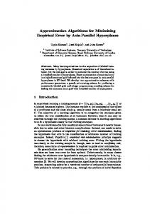
rL r
te n
ta c
le
core subtree
rR
u
uR
uL
uD
Figure 1: On the left, an example of a skeleton tree T . The core subtree of T has depth 2 and two tentacles, one of length 2 and one of length 1. On the right, the corresponding graph GT . explain how to extend it to the asymptotic ratio. The lower bound is established by showing, for any constant R < 6, an adversary strategy for constructing an input graph on which the optimal profit is at least R times the profit of A. Fix some R < 6 and let D be a non-negative integer (that depends on R) whose value will be specified later. It is convenient to describe the graph constructed by the adversary in terms of its underlying skeleton tree T , which is a rooted binary tree. The root of T will be denoted by r. For a node v ∈ T , define the depth or level of v to be the number of edges on the simple path from v to r. The adversary will only use skeleton trees of the following special form: each non-leaf node at depths 0, 1, . . . , D − 1 has two children, and each non-leaf node at levels at least D has one child. Such a tree can be thought of as consisting of its core subtree, which is a complete binary tree of depth D, with paths attached to its leaves at level D. The nodes of T at depth D are the leaves of the core subtree. If v is a node of the core subtree of T then the path extending from v down to a leaf of T is called a tentacle – see Figure 1. (Thus v belongs both to the core subtree and to a tentacle attached to v.) The length of a tentacle is the number of its edges. The nodes in the tentacles are all considered left children of their parents. The graph represented by a skeleton tree T will be denoted by GT . We differentiate between the nodes of T and the vertices of GT . The relation between T and GT is illustrated in Figure 1. GT is obtained from T as follows: • For each node u ∈ T we create two vertices uL and uR in GT , with an edge between them. This edge (uL , uR ) is called the cross edge corresponding to u. • Suppose that u, v ∈ T . If u is in the left subtree of v then (uL , v L ) and (uR , v L ) are edges of GT . If u is in the right subtree of v then (uL , v R ) and (uR , v R ) are edges of GT . These edges are called upward edges. • If u ∈ T is a node in a tentacle of T and is not a leaf, then GT has a vertex uD with edge (uD , uR ). This edge is called a whisker. The adversary constructs GT gradually, in response to A’s choices. Initially, T is a single node r, and thus GT is a single edge (rL , rR ). At this time, profitA (T ) = 0 and O(T ) = 1, so A is forced to collect this edge (that is, it creates a 2-clique {rL , rR }). 7
GT
depth(u) < D
uL uL
depth(u) ≥ D
uR
uR
uL
uR
Figure 2: Adversary moves. Upward edges from new vertices are not shown, to avoid clutter. Dashed lines represent cross edges that are not collected by A, while thick lines represent those that are already collected by A. In general, the algorithm will be able to collect only cross edges. Suppose that, at some step, A collects a cross edge (uL , uR ), corresponding to node u of T . If u is at depth less than D, the adversary extends T by adding two children of u. If u is at depth at least D, the adversary only adds the left child of u, thus extending the tentacle ending at u. In terms of GT , the first move adds two triangles to uL and uR , with all corresponding upward edges. The second move adds a triangle to uL and a whisker to uR (see Figure 2). Thus the adversary will be building the core binary skeleton tree down to level D, and from then on, it will extend the tentacles. Our objective is to prove that after each step the ratio between the adversary profit and the algorithm’s profit is at least 6 − O(1/D). This is enough to prove the lower bound. The reason is this: If the algorithm stops collecting edges at some point, the ratio is 6 − O(1/D), and we are done. Otherwise, suppose that the game lasts for a very long time, and since D is fixed, then at least one tentacle will grow without bound. But the optimal cost is at least quadratic with respect to the maximum tentacle length s, while A’s profit is only linear in s. Thus eventually the adversary can simply stop playing, and even if the algorithm collects the remaining cross edges (and there will be at most 2D · s of those), the ratio will be larger than 6. To simplify the computation of the adversary (or optimal) profit, we will assume that the adversary computes his clustering recursively, as follows: (opt1) If x is a leaf of T , then xL and xR are in the same cluster. (opt2) Suppose that x is an internal node of T and let y be the left child of x. Assume that the clustering of Ty is already computed. If x has a right child, let z be this child and assume that the clustering of Tz is already computed. Then (opt2.a) xL is added either to the cluster of Ty containing y L or to the cluster containing y R . (When we estimate the adversary profit, we will specify which choice we use.) This is correct, since all neighbors of y L and y R that correspond to nodes in Ty are also neighbors of xL . Note that in the special case when y is a leaf, the clusters of y L and y R are the same. (opt2.b) If x has the right child z, then the rule for adding xR to the clustering of Tz is 8
symmetric to (opt2.a). If x does not have the right child (so x is in a tentacle), then we create the “whisker” cluster consisting of two vertices xR and xD . Observe that, in particular, all clusters, except for the whisker clusters, have at least three vertices. We stress that the profit of the clustering computed as above (even for the way we specify the adversary choices in (opt2.a) and (opt2.b)) may not be actually maximized, but this does not matter, since for the purpose of our proof we only need a lower bound on the adversary profit. We now claim that before the core tree reaches its target height D the ratio is at least 6. Indeed, consider one step, when A collects an edge (uL , uR ). (See Figure 2.) The algorithm’s profit increases by 1. As for the adversary, he can increase his profit as follows: (i) Create a new clique that is a triangle consisting of uR and two new vertices, increasing the profit by 3. (ii) In the current clique that contained uL and uR , replace uR by the two new vertices connected to uL . This current clique had size at least 3 (the adversary will maintain the invariant that in his clustering each cross edge is in a clique of size at least 3) and its size increases by 1, so its profit increases by at least 3. Overall, the adversary’s profit increases by at least 6, proving the claim. Thus from now on it is sufficient to analyze skeleton trees of height strictly larger than D, namely trees that have at least one tentacle already started. Let T be such a skeleton tree. Denote by Tv the subtree of T rooted at v. We will focus on analyzing the profits of the adversary and the algorithm on such trees Tv , where v is a node in the core subtree of T . If Tv ends at depth D + 1 or more, we call it a bottom subtree. The core depth of a bottom subtree Tv is defined as the depth of the part of Tv within the core subtree of T . If h and s are, respectively, the core depth of Tv and its maximum tentacle length, then 0 ≤ h ≤ D and s ≥ 1. For a subtree X = Tv , let O(X) be the optimal profit in X, computed according to the description above, and A(X) be A’s profit (the number of cross edges). The lemma below is key in our argument. Lemma 1. Let X be a bottom subtree of height h ≥ 0 and maximum tentacle length s ≥ 1. Then O(X) + 2(h + s) ≥ 6 · A(X). Before proving the lemma, let us argue first that this lemma is sufficient to establish our lower bound. Indeed, since we are now considering the case when T is a bottom subtree itself, the lemma implies that O(T ) + 2(D + s) ≥ 6 · A(T ), where s is the maximum tentacle length of T . But O(T ) is at least quadratic in D + s. So for large D the ratio O(T )/A(T ) approaches 6. So now we prove Lemma 1. The proof is by induction on h, the core height of X. Consider first the base case, for h = 0 (when X is just a tentacle). The adversary has one clique of s + 2 vertices, namely all xL vertices in the tentacle (there are s �+ 1 of these), plus one z R vertex for the leaf z. He also has s whiskers, so his profit for X is s+2 + s = 12 (s2 + 5s + 2). The algorithm 2 collects only s cross edges, namely all cross edges in X except last. (See Figure 3.) Solving the quadratic inequality and using the integrality of s, we get O(X) + 2s ≥≥ 6s = 6 · A(X). Note that this inequality is in fact tight for s = 1, 2. In the inductive step, consider a bottom subtree X = Tu . Let Y and Z be its left and right subtrees, respectively. Without loss of generality, we can assume that Y is a bottom tree with 9
xL
xR
Figure 3: Illustration of the inductive proof, the base case. Subtree X on the left, the corresponding subgraph on the right. height h − 1 and the same maximum tentacle length s as X, while Z is either not a bottom tree (that is, it has no tentacles), or it is a bottom tree with maximum tentacle length at most s.
X u
Y
GX
uL
Z
uR
GZ GY
Figure 4: Illustration of the inductive proof, the inductive step. Subtrees X, Y, Z on the left, the corresponding subgraphs on the right. By the inductive assumption, we have O(Y ) + 2(h − 1 + s) ≥ 6 · A(Y ). Regarding Z, if Z is not a bottom tree then O(Z) ≥ 6 · A(Z), and if Z is a bottom tree (necessarily of height h − 1) then O(Z) + 2(h − 1 + s0 ) ≥ 6 · A(Z), where s0 is Z’s maximum tentacle length, such that 1 ≤ s0 ≤ s. Consider first the case when Z is not a bottom tree. Note that A(X) = A(Y ) + A(Z) + 1 O(X) ≥ O(Y ) + O(Z) + h + s + 4 The first equation is trivial, because for X the algorithm gets all cross edges in Y and Z, plus one more cross edge (uL , uR ). The second inequality holds because uL can be added to Y ’s largest 10
cluster which has (h − 1) + s + 2 = h + s + 1 vertices, and uR can be added to Z’s largest cluster that has at least 3 vertices. Then we get (since h, s ≥ 1): O(X) + 2(h + s) ≥ [O(Y ) + O(Z) + h + s + 4] + 2(h + s) = [O(Y ) + 2(h − 1 + s)] + O(Z) + 6 ≥ 6 · A(Y ) + 6 · A(Z) + 6 = 6 · A(X). The second case is when Z is a bottom tree (of the same core height h − 1) and maximum tentacle length s0 , where 1 ≤ s0 ≤ s. As before, we have A(X) = A(Y ) + A(Z) + 1. The optimum profit satisfies (by a similar argument as before. applied to both Y and Z): O(X) ≥ O(Y ) + O(Z) + 2h + s + s0 + 2. Then we get (using s ≥ s0 ): O(X) + 2(h + s) ≥ [O(Y ) + O(Z) + 2h + s + s0 + 2] + 2(h + s) ≥ [O(Y ) + 2(h − 1 + s)] + [O(Z) + 2(h − 1 + s0 )] + 6 ≥ 6 · A(Y ) + 6 · A(Z) + 6 = 6 · A(X). This completes the proof of Lemma 1, for the case of the absolute competitive ratio. We still need to explain how to extend our proof so that it also applies to the asymptotic competitive ratio. This is quite simple: Choose some large constant M . The adversary will create M instances of the above game, playing each one independently. Our construction above used the fact that at each step the algorithm was forced to collect one of the pending cross edges, for otherwise its competitive ratio would exceed ratio R (where R was arbitrarily close to 6). Now, for M sufficiently large, the algorithm will be forced to collect cross edges in all except for some finite number of copies of the game, where this number depends on the additive constant in the competitiveness bound. Note: Our construction is very tight, in the following sense. Suppose that the algorithm maintains T as balanced as possible. Then the ratio is exactly 6 when the depth of T is 1 or 2. Further, suppose that D is very large and the algorithm constructs T to have depth D or more. Then the ratio is 6 − o(1) for s = 1 and s = 2. The intuition is that when the adversary plays optimally, he will only allow the online algorithm to collect isolated edges (cliques of size 2). For this reason, we conjecture that 6 is the optimal competitive ratio.
References [1] Nikhil Bansal, Avrim Blum, and Shuchi Chawla. Correlation clustering. Machine Learning, 56(1-3):89–113, 2004. [2] Amir Ben-Dor, Ron Shamir, and Zohar Yakhini. Clustering gene expression patterns. Journal of Computational Biology, 6(3/4):281–297, 1999. [3] Moses Charikar, Chandra Chekuri, Tom´as Feder, and Rajeev Motwani. Incremental clustering and dynamic information retrieval. SIAM J. Comput., 33(6):1417–1440, 2004. [4] Marek Chrobak and Claire Kenyon-Mathieu. SIGACT news online algorithms column 10: competitiveness via doubling. SIGACT News, 37(4):115–126, 2006. 11
[5] Anders Dessmark, Jesper Jansson, Andrzej Lingas, Eva-Marta Lundell, and Mia Persson. On the approximability of maximum and minimum edge clique partition problems. Int. J. Found. Comput. Sci., 18(2):217–226, 2007. [6] Aleksander Fabijan, Bengt J. Nilsson, and Mia Persson. Competitive online clique clustering. In Proc. 8th International Conference on Algorithms and Complexity (CIAC’13), pages 221–233, 2013. [7] Andres Figueroa, James Borneman, and Tao Jiang. Clustering binary fingerprint vectors with missing values for DNA array data analysis. Journal of Computational Biology, 11(5):887–901, 2004. [8] Claire Mathieu, Ocan Sankur, and Warren Schudy. Online correlation clustering. In 27th International Symposium on Theoretical Aspects of Computer Science (STACS’10), pages 573– 584, 2010. [9] Lea Valinsky, Gianluca Della Vedova, Ra J. Scupham, Sam Alvey, Andres Figueroa, Bei Yin, R. Jack Hartin, Marek Chrobak, David E. Crowley, Tao Jiang, and James Borneman. Analysis of bacterial community composition by oligonucleotide fingerprinting of rRNA genes. Applied and Environmental Microbiology, 68:2002, 2002.
12
A
A Technical Lemma
Lemma 2. For any pair of non-negative integers a and b, the inequality � � � � � � a+b a x+1 b ≤ (x + 1) + +a 2 2 x 2 holds for any 0 < x ≤ 1. Proof. Define the function � � � � � � a b a+b F (a, b, x) = 2x(x + 1) + 2(x + 1) + 2ax − 2x 2 2 2 = a2 x2 − ax2 + 2ax + b2 − b − 2abx = (b − ax)2 + ax(2 − x) − b. It is sufficient to show that F (a, b, x) is non-negative for integers a, b ≥ 0 and 0 < x ≤ 1 to prove the lemma. Consider first the cases when a = {0, 1} or b = {0, 1}. F (0, b, x) = b(b − 1) ≥ 0, for any non-negative integer b and any x. F (a, 0, x) = ax(ax − x + 2) ≥ ax(ax + 1) > 0, for any positive integer a and 0 < x ≤ 1. F (a, 1, x) = x2 a(a − 1) ≥ 0, for any positive integer a and any x. F (1, 2, x) = 2 − 2x ≥ 0, for 0 < x ≤ 1, and F (1, b, x) = b2 − b + 2x − 2bx ≥ b2 − 3b ≥ 0, for any integer b ≥ 3 and 0 < x ≤ 1. Thus, it only remains to show that F (a, b, x) is non-negative when both a ≥ 2 and b ≥ 2. b−1 The function F (a, b, x) has a local minimum in x at x = a−1 , as can be easily verified by differentiating F in x. Therefore, in the case when a ≤ b, F (a, b, x) ≥ F (a, b, 1) = (b−a)2 −(b−a) ≥ b−1 )= (b − a) − (b − a) = 0, for 0 < x ≤ 1. In the case when a > b, we have that F (a, b, x) ≥ F (a, b, a−1 (a−b)(b−1) a−1
B
> 0, which completes the proof.
A Lower Bound for Algorithm OCC
In this subsection we will show that, for any choice of γ, the worst-case ratio of Algorithm OCC is at least 10.927. Denote by Bj the j-th batch. We will use notation Aj for the profit of OCC and Oj for the optimal profit on the sub-instance consisting of the first j batches. To avoid clutter we will omit lower order terms in our calculations. In particular, we focus on j large enough, treating γ j as integer, and all estimates for Aj and Oj given below are meant to hold within a factor of 1 ± o(1). We start with a simpler construction that shows a lower bound of 9; then later we will explain how to improve it to 10.927. In the instance we construct, all batches will be disjoint, with the jth batch Bj having 2γ j vertices connected by γ j disjoint edges (that is, a perfect matching). We will refer to these edges as batch edges. The edges between any two batches Bi and Bj , for i < j, form a complete bipartite graph. These edges will be called cross edges. At the end of each phase j, the algorithm will collect all γ j edges inside Bj . Therefore, by summing up the geometric sequence, right before the end of phase j (before the algorithm adds the new edges from Bj to its clustering), the algorithm’s profit is Aj =
j−1 X
γi ≤
i=0
13
γj . γ−1
...
...
...
Figure 5: Bad example for Algorithm OCC. The figure shows two batches Bi and Bj , for i < j. Batch edges, drawn with solid lines, are collected by Algorithm OCC. Dotted lines show cross edges that are in the adversary’s clustering. Shaded regions illustrate the cliques in the adversary’s clustering. After the first j phases, the adversary’s clustering consists of cliques Cp , p = 0, 1, ..., γ j − 1, where Cp contains the p-th edge (that is, its both endpoints) from each batch Bi for i = p, p + 1, ..., j. (See Figure 5.) We claim that the adversary gain after j phases satisfies j
Oj ≥ Oj−1 + γ + 4
j−1 X
γ i = Oj−1 +
i=0
(γ + 3)γ j . γ−1
(13)
We now justify this bound. The second term γ j is simply the number of batch edges in Bj . To see where each term 4γ i comes from, consider the p-th batch edge from Bi , for i < j. When we add Bj after phase j, the adversary can add to Cp the 4 cross edges connecting this edge’s endpoints to the endpoints of the pth batch edge in Bj . Overall, this will add 4γ i cross edges between Bi and Bj to the existing adversary’s cliques. From recurrence (13), by simple summation, we get Oj ≥
(γ + 3)γ j+1 . (γ − 1)2
Dividing it by OCC’s profit of at most γ j /(γ − 1), we obtain that the ratio is at least γ(γ+3) γ−1 , which, by routine calculus, is at least 9. We now outline an argument showing how to improve this lower bound to 10.927. The new construction is almost identical to the previous one, except that we change the very last batch Bj . As before, each batch Bi , for i < j, has γ i disjoint edges. Batch Bj will also have γ j edges, but they will be grouped into t = γ j /3 triangles. For p = 0, 1, ..., t − 1, we add the p-th triangle to clique Cp . (If t > γ j−1 , the last t − γ j−1 triangles will form new cliques.) This modification will preserve the number of edges in Bj and thus it will not affect the algorithm’s profit. But now, for each i = 0, 1, ..., j − 1 and each p = 0, 1, ..., min(t, γ i−1 ) − 1, we can connect the two vertices in Bi ∩ Cp to three vertices in Bj , instead of two. This creates two new cross edges that will be called extra edges. It should be intuitively clear that the number of these extra edges is Ω(γ j ), which means that this new construction gives a ratio strictly larger than 9. 14
Specifically, to estimate the ratio, we will distinguish three cases, depending of γ. Pj−1 oni the value j−1 j Suppose first that γ ≥ 3. Then t ≥ γ , so the number of extra edges is 2 i=0 γ = 2γ /(γ − 1), because each vertex in B0 ∪ B1 ∪ ... ∪ Bj−1 is now connected to three vertices in Bj , not two. Thus the new optimal profit is 2γ j (γ 2 + 5γ − 2)γ j . O0j = Oj + = γ−1 (γ − 1)2 2
Dividing by OCC’s profit, the ratio is at least γ +5γ−2 γ−1 , which is at least 11 for γ ≥ 3. √ The second case is when 3 ≤ γ ≤ 3. Then γ j−2 ≤ t ≤ γ j−1 . In this case all vertices in B0 ∪ B1 ∪ ... ∪ Bj−2 and 2γ j /3 vertices in Bj−1 get an extra edge, so the number of extra edges is 2γ j−1 /(γ − 1) + 2γ j /3. Therefore the new adversary profit is O0j = Oj + 2
γ j−1 (5γ 3 + 5γ 2 + 8γ − 6)γ j−1 + 23 γ j = . γ−1 3(γ − 1)2 3
2
+8γ−6 . Minimizing this quantity, we obtain that the We thus have that the ratio is at least 5γ +5γ 3γ(γ−1) ratio is at least 10.927. √ The last case is when 1 < γ ≤ 3. In√this case, even ignoring the extra edges, we have that the √ is at least 3 + 6 ratio Oj /Aj−1 = γ(γ+3) 3 ≈ 11.2 (it is minimized for γ = 3). γ−1
15