Mar 31, 2014 - resources (such as buffer space, hard disk space, I/O band- width, and number .... PQO problem into several SOQO problems [10, 15, 5] by fix-.
Approximation Schemes for Many-Objective Query Optimization Immanuel Trummer and Christoph Koch École Polytechnique Fédérale de Lausanne
{firstname}.{lastname}@epfl.ch
arXiv:1404.0046v1 [cs.DB] 31 Mar 2014
ABSTRACT The goal of multi-objective query optimization (MOQO) is to find query plans that realize a good compromise between conflicting objectives such as minimizing execution time and minimizing monetary fees in a Cloud scenario. A previously proposed exhaustive MOQO algorithm needs hours to optimize even simple TPC-H queries. This is why we propose several approximation schemes for MOQO that generate guaranteed near-optimal plans in seconds where exhaustive optimization takes hours. We integrated all MOQO algorithms into the Postgres optimizer and present experimental results for TPC-H queries; we extended the Postgres cost model and optimize for up to nine conflicting objectives in our experiments. The proposed algorithms are based on a formal analysis of typical cost functions that occur in the context of MOQO. We identify properties that hold for a broad range of objectives and can be exploited for the design of future MOQO algorithms.
1.
INTRODUCTION
Minimizing execution time is the only objective in classical query optimization [22]. Nowadays, there are however many scenarios in which additional objectives are of interest that should be considered during query optimization. This leads to the problem of multi-objective query optimization (MOQO) in which the goal is to find a query plan that realizes the best compromise between conflicting objectives. Consider the following example scenarios. Scenario 1. A Cloud provider lets users submit SQL queries on data that resides in the Cloud. Queries are processed in the Cloud and users are billed according to the accumulated processing time over all nodes that participated in processing a certain query. The processing time of aggregation queries can be reduced by using sampling but this has a negative impact on result quality. From the perspective of the users, this leads to the three conflicting objectives of minimizing execution time, minimizing monetary costs,
and minimizing the loss in result quality. Users specify preferences in their profiles by setting weights on different objectives, representing relative importance, and by optionally specifying constraints (e.g., an upper bound on execution time). Upon reception of a query, the Cloud provider needs to find a query plan that meets all constraints while minimizing the weighted sum over different cost metrics. Scenario 2. A powerful server processes queries of multiple users concurrently. Minimizing the amount of system resources (such as buffer space, hard disk space, I/O bandwidth, and number of cores) that are dedicated for processing one specific query and minimizing that query’s execution time are conflicting objectives (each specific system resource would correspond to an objective on its own). Upon reception of a query, the system must find a query plan that represents the best compromise between all conflicting objectives, considering weights and bounds defined by an administrator. The main contribution in this paper are several MOQO algorithms that are generic enough to be applicable in a variety of scenarios (including the two scenarios outlined above) and are much more efficient than prior approaches while they formally guarantee to generate near-optimal query plans.
1.1
State of the Art
The goal of MOQO, according to our problem model, is to find query plans that minimize a weighted sum over different cost metrics while respecting all cost bounds. This means that multiple cost metrics are finally combined into a single metric (the weighted sum); it is still not possible to reduce MOQO to single-objective query optimization and use classic optimization algorithms such as the one by Selinger [22]. Ganguly et al. have thoroughly justified why this is not possible [11]; we quickly outline the reasons in the following. Algorithms that prune plans based on a single cost metric must rely on the single-objective principle of optimality: replacing subplans (e.g., plans generating join operands) within a query plan by subplans that are better according to that cost metric cannot worsen the entire query plan according to that metric. This principle breaks when the cost metric of interest is a weighted sum over multiple metrics that are calculated according to diverse cost formulas. Example 1. Assume that each query plan is associated with a two-dimensional cost vector of the form (t, e) where t represents execution time in seconds and e represents energy consumption in Joule. Assume one wants to minimize the weighted sum over time and energy with weight 1 for time
and weight 2 for energy, i.e. the sum t + 2e. Let p be a plan that executes two subplans p1 with cost vector (7, 1) and p2 with cost vector (6, 2) in parallel. The cost vector of p is (7, 3) since its execution time is the maximum over the execution times of its subplans (7 = max(7, 6)) while its energy consumption is the sum of the energy consumptions of its subplans (3 = 1 + 2). Replacing p1 within p by another plan p01 with cost vector (1, 3) changes the cost vector of p from (7, 3) to (6, 5). This means that the weighted cost of p becomes worse (it increases from 13 to 16) even if the weighted cost of p01 (7) is better than the one of p1 (9). The example shows that the single-objective principle of optimality can break when optimizing a weighted sum of multiple cost metrics. Based on that insight, Ganguly et al. proposed a MOQO algorithm that uses a multi-objective version of the principle of optimality [11]. This algorithm guarantees to generate optimal query plans; it is however too computationally expensive for practical use as we will show in our experiments. The algorithm by Ganguly et al. is the only MOQO algorithm that we are aware of which is generic enough to handle all objectives that were mentioned in the example scenarios before. Most existing MOQO algorithms are specific to certain combinations of objectives where the single-objective principle of optimality holds [2, 27, 16].
1.2
Contributions and Outline
We summarize our contributions before we provide details: • Our primary contribution are two approximation schemes for MOQO that scale to many objectives. They formally guarantee to return near-optimal query plans while speeding up optimization by several orders of magnitude in comparison with exact algorithms. • We formally analyze cost formulas of many relevant objectives in query optimization and derive several common properties. We exploit these properties to design efficient approximation schemes and believe that our observations can serve as starting point for the design of future MOQO algorithms. • We integrated the exact MOQO algorithm by Ganguly et al. [11] and our own MOQO approximation algorithms into the Postgres optimizer and experimentally compare their performance on TPC-H queries. Our approximation schemes formally guarantee to generate query plans whose cost is within a multiplicative factor α of the optimum in each objective. Parameter α can be tuned seamlessly to trade near-optimality guarantees for lower computational optimization cost. The near-optimality guarantees distinguish our approximation schemes from heuristics, since heuristics can produce arbitrarily poor plans in the worst case. We show in our experimental evaluation that our approximation schemes reduce query optimization time from hours to seconds, comparing with an existing exact MOQO algorithm proposed by Ganguly et al. that is referred to as the EXA in the following. We discuss related work in Section 2 and introduce the formal model in Section 3. Our experimental evaluation is based on an extended version of Postgres that we describe in Section 4. Note that our algorithms for MOQO are not specific to Postgres and can be used within any database
system. We present the first experimental evaluation of the formerly proposed EXA in Section 5. Our experiments relate the poor scalability of the EXA to the high number of Pareto plans (i.e., plans representing an optimal tradeoff between different cost objectives) that it needs to generate. The representative-tradeoffs algorithm (RTA), that we present in Section 6, generates only one representative for multiple Pareto plans with similar cost tradeoffs and is therefore much more efficient than the EXA. We show that most common objectives in MOQO allow to construct near-optimal plans for joining a set of tables out of near-optimal plans for joining subsets. Due to that property, the RTA formally guarantees to generate near-optimal query plans if user preferences are expressed by associating objectives with weights (representing relative importance). If users can specify cost bounds in addition to weights (representing for instance a monetary budget or a deadline), the RTA cannot guarantee to generate near-optimal plans anymore and needs to be extended. We present the iterative-refinement algorithm (IRA) in Section 7. The IRA uses the RTA to generate a representative plan set in every iteration. The approximation precision is refined from one iteration to the next such that the representative plan set resembles more and more the Pareto plan set. The IRA stops once it can guarantee that the generated plan set contains a near-optimal plan. A carefully selected precision refinement policy guarantees that the amount of redundant work (by repeatedly generating the same plans in different iterations) is negligible. We analyze time and space complexity of all presented algorithms and experimentally compare our two approximation schemes (the RTA and the IRA) against the EXA in Section 8.
2.
RELATED WORK
Algorithms for Single-Objective Query Optimization (SOQO) are not applicable to MOQO or cannot offer any guarantees on result quality. Selinger et al. [22] presented one of the first exact algorithms for SOQO which is based on dynamic programming. Multi-Objective Query Optimization is the focus of this paper. The algorithm by Ganguly et al. [11] is a generalization of the SOQO algorithm by Selinger et al. This algorithm is able to generate optimal query plans considering a multitude of objectives with diverse cost formulas. We describe it in more detail later, as we use it as baseline for our experiments. Algorithms for MOQO have not been experimentally evaluated for more than three objectives. They are usually tailored to very specific combinations of objectives. Neither the proposed algorithms nor the underlying algorithmic ideas can be used for many-objective QO with diverse cost formulas. Allowing only additive cost formulas (and user preference functions) [27, 16] excludes for instance run time as objective in parallel execution scenarios (where time is calculated as maximum over parallel branches). The approach by Aggarwal et al. [2] is specific to the two objectives run time and confidence. Multiple objectives are only considered by selecting an optimal set of table samples prior to join ordering which does not generalize to different objectives. Optimizing different objectives separately misses optimal tradeoffs between conflicting objectives [1]. Separating join ordering and multi-objective optimization (e.g., by generating a time-optimal join tree first, and mapping join operators to sites considering multiple objectives later [12, 21]) assumes that the same join tree is optimal for all ob-
3.
FORMAL MODEL
We represent queries as set of tables Q that need to be joined. This model abstracts away details such as join predicates (that are however considered in the implementations of the presented algorithms). Query plans are characterized by the join order and the applied join and scan operators, chosen out of a set J of available operators. The two plans generating the inputs for the final join in a query plan p are the sub-plans of p. The set O contains all cost objectives (e.g., O = {buffer space, execution time}); we assume that a cost model is available for every objective that allows to estimate the cost of a plan. The function c(p) denotes the multi-dimensional cost of a plan p (bold font distinguishes vectors from scalar values). Cost values are real-valued and non-negative. Let o ∈ O an objective, then co denotes the cost for o within vector c. Let W a vector P of onon-negative o weights, then the function CW (c) = o∈O c W denotes the weighted cost of c. Let B a vector of non-negative bounds (setting Bo = ∞ means no bounds), then cost vector c exceeds the bounds if there is at least one objective o with co > Bo . Vector c respects the bounds otherwise. The following two variants of the MOQO problem distin-
3
3
2
2
Time
Time
jectives. This is only valid in special cases. Papadimitriou and Yannakakis [21] present multi-objective approximation algorithms for mapping operators to sites. Their algorithms do not optimize join order and the underlying approach does not generalize to more than one bounded objective. Algorithms for multi-objective optimization of data processing workflows [23, 24, 17] are not directly applicable to MOQO. Furthermore, the proposed approaches can be classified into heuristics that do not offer near-optimality guarantees [24, 17], and exact algorithms that do not scale [23]. Parametric Query Optimization (PQO) assumes that cost formulas depend on parameters with uncertain values. The goal is for instance to find robust plans [4, 3] or plans that optimize expected cost [7]. PQO and MOQO share certain problem properties while subtle differences prevent us from applying PQO algorithms to MOQO problems in general. Several approaches to PQO split for instance the PQO problem into several SOQO problems [10, 15, 5] by fixing parameter values. This is not possible for MOQO since cost values, unlike parameter values, are only known once a query plan is complete and cannot be fixed in advance. Other PQO algorithms [15] directly work with cost functions instead of scalar values during bottom-up plan construction. This assumes that all parameter values can be selected out of a connected interval which is typically not the case for cost objectives such as time or disc footprint. Our work connects to Iterative Query Optimization since we propose iterative algorithms. Kossmann and Stocker [19] propose several iterative algorithms that break the optimization of a large table set into multiple optimization runs for smaller table sets, thereby increasing efficiency. Their algorithm is only applicable to SOQO and does not offer formal guarantees on result quality. Work on Skyline Queries [18] and Optimization Queries [13] focuses on query processing while we focus on query optimization. Our work is situated in the broader area of Approximation Algorithms. We use generic techniques such as coarsening that have been applied to other optimization problems [8, 20]; the corresponding algorithms are however not applicable to query optimization and the specific coarsening methods differ.
1 0
0
1 2 3 Buffer Space
4
(a) Weighted MOQO
Plan Cost
Weights
1 0
0
1 2 3 Buffer Space
4
(b) Bounded-Weighted MOQO
Bounds
Optimal Cost
Figure 1: The two MOQO problem variants guish themselves by the expressiveness of the user preference model. Definition 1. Weighted MOQO Problem. A weighted MOQO problem instance is defined by a tuple I = hQ, Wi where Q is a query and W a weight vector. A solution is a query plan for Q. An optimal plan minimizes the weighted cost CW over all plans for Q. Definition 2. Bounded-Weighted MOQO Problem. A bounded-weighted MOQO problem instance is defined by a tuple I = hQ, W, Bi and extends the weighted MOQO problem by a bounds vector B. Let P the set of plans for Q and PB ⊆ P the set of plans that respect B. If PB is nonempty, an optimal plan minimizes CW among the plans in PB . If PB is empty, an optimal plan minimizes CW among the plans in P . Figure 1(a) illustrates weighted MOQO. It shows cost vectors of possible query plans (considering time and buffer space as objectives) and the user-specified weights (as vector from the origin). The line orthogonal to the weight vector represents cost vectors of equal weighted cost. The optimal plan is found by shifting this line to the top until it touches the first plan cost vector. Figure 1(b) illustrates boundedweighted MOQO. Additional cost bounds are specified and a different plan is optimal since the formerly optimal plan exceeds the bounds. We will use the set of cost vectors depicted in Figure 1 as running example throughout the paper. The relative cost function ρ measures the cost of a plan relative to an optimal plan. Definition 3. Relative Cost. The relative cost function ρI of a weighted MOQO instance I = hQ, Wi judges a query plan p by comparing its weighted cost to the one of an optimal plan p∗ : ρI (p) = CW (c(p))/CW (c(p∗ )). The relative cost function of a bounded-weighted MOQO instance I = hQ, W, Bi is defined in the same way if no plan exists that respects B. Otherwise, set ρI (p) = ∞ for any plan p that does not respect B and ρI (p) = CW (c(p))/CW (c(p∗ )) if p respects B. Let α ≥ 1, then an α-approximate solution to a weighted MOQO or bounded-weighted MOQO instance I is a plan p whose relative cost is bounded by α: ρI (p) ≤ α. The following classification of MOQO algorithms is based on the formal near-optimality guarantees that they offer. Definition 4. MOQO Approximation Scheme. An approximation scheme for MOQO is tuned via a user-specified precision parameter αU and guarantees to generate an αU approximate solution for any MOQO problem instance.
Time
4 Plan Cost Pareto Frontier Dominated Area
2 0
0
2 4 Buffer Space Figure 2: Pareto frontier and dominated area Definition 5. Exact MOQO Algorithm. An exact algorithm for MOQO guarantees to generate a 1-approximate (hence optimal) solution for any MOQO problem instance. The following definitions express relationships between cost vectors. A vector c1 dominates vector c2 , denoted by c1 � c2 , if c1 has lower or equivalent cost than c2 in every objective. Vector c1 strictly dominates c2 , denoted by c1 ≺ c2 , if c1 � c2 and the vectors are not equivalent (c1 6= c2 ). Vector c1 approximately dominates c2 with precision α, denoted by c1 �α c2 , if the cost of c1 is higher at most by factor α in every objective, i.e. ∀o : co1 ≤ co2 · α. A plan p and its cost vector are Pareto-optimal for query Q (short: Pareto plan and Pareto vector) if no alternative plan for Q strictly dominates p. A Pareto set for Q contains at least one cost-equivalent plan for each Pareto plan. The Pareto frontier is the set of all Pareto vectors. Figure 2 shows the Pareto frontier of the running example and the area that each Pareto vector dominates. An α-approximate Pareto set for Q contains for every Pareto plan p∗ a plan p such that c(p) �α c(p∗ ). An αapproximate Pareto frontier contains the cost vectors of all plans in an α-approximate Pareto set. During complexity analysis, j = |J| denotes the number of operators, l = |O| the number of objectives, n = |Q| the number of tables to join, and m the maximal cardinality over all base tables in the database. Users formulate queries and have direct influence on table cardinalities. Therefore, n and m (and also j) are treated as variables during asymptotic analysis. Introducing new objectives (that cannot be derived from existing ones) requires changes to the code base and detailed experimental analysis to provide realistic cost formulas. This is typically not done by users, therefore l is treated as a constant (it is common to treat the number of objectives as a constant when analyzing multi-objective approximation schemes [21, 8]).
4.
PROTOTYPICAL IMPLEMENTATION
We extended the Postgres system (version 9.2.4) to obtain an experimental platform for comparing MOQO algorithms. We extended the cost model, the query optimizer, and the user interface. The extended cost model supports nine objectives. The cost formulas used in the cost model are taken from prior work and are not part of our contribution. Evaluating their accuracy is beyond the scope of this paper. We quickly describe the nine implemented cost objectives. Total execution time (i.e., time until all result tuples have been produced) and startup time (i.e., time until first result tuple is produced) are estimated according to the cost formulas already included in Postgres. Minimizing IO load, CPU load, number of used cores, hard disc footprint, and buffer footprint is important since it allows to increase the number of concurrent users. The
L=Lineitem; O=Orders; C=Customers; HashJ=Hash Join; SMJ=Sort-Merge Join; IdxNL=Index-Nested-Loop Join HashJ 1 L
HashJ 1 O C
(a) Time-Optimal Plan for Bounded Tuple Loss (= 0)
SMJ 1 L
IdxNL 1 O C
(b) Additional Weight on Buffer Space Leads to Plan Without Hash Joins
IdxNL 1 IdxNL C 1 L O (c) Additional Bound on Startup Time Requires Using Nested-Loop Joins
Figure 3: Evolution of optimal plan for TPC-H Query 3 when changing user preferences
five aforementioned objectives often conflict with run time since using more system resources can often speed up query processing. Energy consumption is not always correlated with time [27, 9]. Dedicating more cores to a query plan can for instance decrease execution time by parallelization while it introduces coordination overhead that results in higher total energy consumption. Energy consumption is calculated according to the cost formulas by Flach [9]. Sampling allows to trade result completeness for efficiency [14]. The tuple loss ratio is the expected fraction of lost result tuples due to sampling and serves as ninth objective. Joining two operands with tuple loss a, b ∈ [0, 1], the tuple loss of the result is estimated by the formula 1 − (1 − a)(1 − b). We extended the plan space of the Postgres optimizer by introducing new operators and parameterizing existing ones (we did not implement those operators in the execution engine). The extended plan space includes a parameterized sampling operator that scans between 1% and 5% of a base table. Join and sort operators are parameterized by the degree of parallelism (DOP). The DOP represents the number of cores that process the corresponding operation (up to 4 cores can be used per operation). The Postgres optimizer uses several heuristics to restrict the search space: in particular, i) it considers Cartesian products only in situations in which no other join is applicable, and ii) it optimizes different subqueries of the same query separately. We left both heuristics in place since removing them might have significant impact on performance. Not using those heuristics would make it difficult to decide whether high computational costs observed during MOQO are due to the use of multiple objectives or to the removal of the heuristics. The original Postgres optimizer is single-objective and optimizes total execution time. We implemented all three MOQO algorithms that are discussed in this paper: the EXA, the RTA, and the IRA. The implementation uses the original Postgres data structures and routines wherever possible. Users can switch between the optimization algorithms and can choose the approximation precision α for the two approximation schemes. Users can specify weights and bounds on the different objectives. The higher the weight on some objective, the higher its relative importance. Bounds allow to specify cost limits for specific objectives (e.g., time limits or energy budgets). When optimizing a query, the optimizer tries to find a plan that minimizes the weighted cost among all plans that respect the bounds. Figure 3 shows how the optimal query plan for TPC-H query 3 changes when user
Time (PG Optimizer Units)
1: // Find best plan for query Q, weights W, bounds B 2: function ExactMOQO(Q, W, B) 3: // Find Pareto plan set for Q 4: P ← FindParetoPlans(Q) 5: // Return best plan out of Pareto plans 6: return SelectBest(P, W, B)
·108 1.5 1 0.5 0 0
0.1 0.2 0.3 0.4 0.5 0.6 0.7 0.8 0.9 Tuple Loss (Fraction )
1 7
6
5
4
3
r ffe Bu
2
1
0
s) ·106 yte (B
Time (PG Optimizer Units)
(a) Coarse-Grained Approximation (α = 2)
·108 1.5 1 0.5 0 0
0.1 0.2 0.3 0.4 0.5 0.6 0.7 0.8 0.9 Tuple Loss (Fraction )
1 7
6
5
4
3
r ffe Bu
2
1
0
s) ·106 yte (B
(b) Fine-Grained Approximation (α = 1.25)
Pareto Surface Interpolation
Single Plan Cost
Figure 4: Three-dimensional Pareto frontier approximations for TPC-H Query 5 preferences vary. Initially, the tuple loss is upper-bounded by zero (i.e., all result tuples must be retrieved) and all weights except the one for total execution time are set to zero. So the optimizer searches for the plan with minimal execution time among all plans that do not use sampling. Figure 3(a) shows the resulting plan. Increasing the weight on buffer footprint leads to a plan that replaces the memoryintensive Hash joins by Sort-Merge and Index-Nested-Loop (IdxNL) joins (see Figure 3(b)). Setting an additional upper bound on startup time leads to a plan that only uses IdxNL joins (see Figure 3(c)). Users cannot make optimal choices for bounds and weights if they are not aware of the possible tradeoffs between different objectives. A user might for instance want to relax the bound on one objective, knowing that this allows significant savings in another objective. All implemented MOQO algorithms produce an (approximate) Pareto frontier as byproduct of optimization. Our prototype allows to visualize two and three dimensional projections of the Pareto frontier. Figure 4 shows the cost vectors of the approximate Pareto frontier for TPC-H query 5 (and an interpolation of the surface defined by those vectors), considering objectives tuple loss, buffer footprint, and total execution time. Figure 4(a) shows a coarse-grained approximation of the real Pareto frontier (with α = 2) and Figure 4(b) a more finegrained approximation for the same query (α = 1.25).
5.
ANALYSIS OF EXACT ALGORITHM
Ganguly et al. [11] proposed an exact algorithm (EXA) for MOQO. This algorithm is not part of our contribution but we provide a first experimental evaluation in a manyobjective scenario and a formal analysis under less optimistic assumptions than in the original publication. Algorithm 1 shows the pseudo-code of the EXA (compared with the orig-
7: // Find Pareto plan set for query Q 8: function FindParetoPlans(Q) 9: // Calculate plans for singleton sets 10: for all q ∈ Q do 11: Pq ← ∅ 12: for all pN access path for q do 13: Prune(P q , pN ) 14: // Consider table sets of increasing cardinality 15: for all k ∈ 2..|Q| do 16: for all q ⊆ Q : |q| = k do 17: Pq ← ∅ 18: // For all possible splits of set q ˙ 2 = q do 19: for all q1 , q2 ⊂ q : q1 ∪q 20: // For all sub-plans and operators 21: for all p1 ∈ P q1 , p2 ∈ P q2 , j ∈ J do 22: // Construct new plan out of sub-plans 23: pN ← Combine(j, p1 , p2 ) 24: // Prune with new plan 25: Prune(P q , pN ) Q 26: return P 27: // Prune plan set P with new plan pN 28: procedure Prune(P, pN ) 29: // Check whether new plan useful 30: if ¬∃p ∈ P : c(p) � c(pN ) then 31: // Delete dominated plans 32: P ← {p ∈ P | ¬(c(pN ) � c(p))} 33: // Insert new plan 34: P ← P ∪ {pN } 35: // Select best plan in P for weights W and bounds B 36: function SelectBest(P, W, B) 37: PB ← {p ∈ P | c(p) � B} 38: if PB 6= ∅ then 39: return arg min[p ∈ PB ]CW (c(p)) 40: else 41: return arg min[p ∈ P ]CW (c(p)) Algorithm 1: Exact algorithm for MOQO inal publication, the code was slightly extended to generate bushy plans in addition to left-deep plans). The EXA first calculates a Pareto plan set for query Q and finally selects the optimal plan out of that set (considering weights and bounds). The EXA uses dynamic programming and constructs Pareto plans for a table set out of the Pareto plans of its subsets. It is a generalization of the seminal algorithm by Selinger et al. [22], generalizing the pruning metric from one to multiple cost objectives. The EXA starts by calculating Pareto plans for single tables. Plans generating the same result are compared and pruned, meaning that dominated plans are discarded. The EXA constructs Pareto plans for table sets of increasing cardinality. To generate plans for a specific table set, the EXA considers i) all possible splits of that set into two non-empty subsets (every split corresponds to one choice of operands for the last join), ii) all available join operators, and iii) all combinations of Pareto plans for generating the two inputs to the last join.
5.1
Experimental Analysis
We implemented the EXA within the system described in Section 4. The implementation allows to specify timeouts (the corresponding code is not shown in Algorithm 1). If
107 Memory (KB)
Time (ms)
Out 106 105 104 103 102 101
105 104 103
1
5000 # Pareto Plans
106
2
3
4
5
6
7
8
# Join Tables 512
1 Objective, No Timeouts 1 Objective, Timeouts
64
3 Objectives, No Timeouts 8
3 Objectives, Timeouts
1
6 Objectives, No Timeouts 1
2
3
4
5
6
# Join Tables
7
8
6 Objectives, Timeouts 9 Objectives, No Timeouts 9 Objectives, Timeouts
Figure 5: Performance of exact algorithm on TPC-H: Prohibitive computational cost due to high number of Pareto plans (timeout at 2 hours) the optimization time exceeds two hours, the modified EXA finishes quickly by only generating one plan for all table sets that have not been treated so far. We experimentally evaluated the EXA using the TPC-H [25] benchmark. We generated several test cases for each TPC-H query by randomly selecting subsets of objectives with a fixed cardinality out of the total set of nine objectives. All experiments were executed on a server equipped with two six core Intel Xeon processors with 2 GhZ and 128 GB of DDR3 RAM running Linux 2.6 (64 bit version). Five optimizer threads ran in parallel during the experiments. The goal of the evaluation was to answer three questions: i) Is the performance of the EXA good enough for use in practice? ii) If not, how can the performance be improved? iii) What assumptions are realistic for the formal complexity analysis of MOQO algorithms? Figure 5 shows experimental results for the three metrics optimization time, allocated memory during optimization, and number of Pareto plans for the last table set that was treated completely (before a timeout occurred or before the optimization was completed). Every marker represents the arithmetic average value over 20 test cases for one specific TPC-H query and a specific number of objectives. The TPC-H queries are ordered according to the maximal number of tables that appears in any of their from-clauses. This number correlates (with several caveats1 ) with the search space size. Gray markers indicate that some test cases incurred a timeout. If a timeout occurred, then the reported values are lower bounds on the values of a completed computation. Optimizing for one objective never requires more than 100 milliseconds per query and never consumes more than 1.7 MB of main memory. For multiple objectives, the computational cost of the EXA becomes however quickly prohibitive with growing number of tables (referring to Question i)). The EXA often reaches the timeout of two hours and allocates gigabytes of main memory during optimization. This happens already for queries joining only three tables; while the number of possible join orders is small in this case, the total search space size is already significant as over 10 different configurations are considered for the scan and for the 1
The Postgres optimizer may for instance convert EXISTS predicates into joins which leads to many alternative plans even for queries with only one table in the from-clause.
join operator respectively (considering for instance different sample densities and different degrees of parallelism). Figure 5 explains the significant difference in time and space requirements between SOQO and MOQO: The number of Pareto plans per table set is always one for SOQO but grows quickly in the number of tables (and objectives) for MOQO. The space consumption of the EXA directly relates to the number of Pareto plans. The run time relates to the total number of considered plans which is much higher than the number of Pareto plans but directly correlated with it2 . Discarding Pareto plans seems therefore the most natural way to increase efficiency (referring to Question ii)). Ganguly et al. [11] used an upper bound of 2l (l designates the number of objectives) on the number of Pareto plans per table set for their complexity analysis of the EXA. This bound derives from the optimistic assumption that different objectives are not correlated. Figure 5 shows that this bound is unrealistic (8, 64, and 512 are the theoretical bounds for 3, 6, and 9 objectives). The bound is a mismatch from the quantitative perspective (as the bound is exceeded by orders of magnitude3 ) and from the qualitative perspective (as the number of Pareto plans seems to correlate with the search space size while the postulated bound only depends on the number of objectives). Therefore, this bound is not used in the following complexity analysis (referring to Question iii)).
5.2
Formal Complexity Analysis
All query plans can be Pareto-optimal in the worst case (when considering at least two objectives). The following analysis remains unchanged under the assumption that a constant fraction of all possible plans is Pareto-optimal. If only one join operator is available, then the number of bushy plans for joining n tables is given by (2(n − 1))!/(n − 1)! [11]. If j scan and join operators are available, then the number of possible plans is given by Nbushy (j, n) = j 2n−1 (2(n − 1))!/(n − 1)!. Theorem 1. The EXA has space complexity O(Nbushy (j, n)). Proof. Plan sets are the variables with dominant space requirements. A scan plan is represented by an operator ID and a table ID. All other plans are represented by the operator ID of the last join and pointers to the two sub-plans generating its operands. Therefore, each stored plan needs only O(1) space. Each stored cost vector needs O(1) space as well, since l is a constant (see Section 3). Let Q the set of tables to join. The EXA stores a set of Pareto plans for each non-empty subset of Q. The total number of stored plans is the sum of Pareto plans over all subsets. Let k ∈ {1, . . . , |Q|} and denote by xk the total number of Pareto plans, summing over all subsets of Q with cardinality k. Each� plan is Pareto-optimal in the worst case, therefore xk = nk Nbushy (j, k). It is xk ≤ 2xk+1 for k > 1. Therefore, the term xn = Nbushy (j, n) dominates. The analysis is tight since the EXA has to store this number of plans in the worst case. 2
All plans considered for joining a set of tables are combinations of two Pareto plans; the number of considered plans therefore grows quadratically in the number of Pareto plans. 3 We generate up to 443 Pareto plans on average when considering three objectives and up to 3157 plans when considering six objectives.
4
2 O(Nbushy (j, n)).
Proof. Every plan is compared with all other plans that generate the same result. So the time complexity grows quadratically in the number of Pareto plans and a similar reasoning as in the proof of Theorem 1 can be applied. The main advantage of the Selinger algorithm for SOQO [22] over a naive plan enumeration approach is that its complexity only depends on the number of table sets but not on the number of possible query plans. The preceding analysis shows that this advantage vanishes when generalizing the Selinger algorithm to multiple cost objectives (leading to the EXA). The complexity of the EXA is even worse than that of an approach that successively generates all possible plans while keeping only the best plan generated so far.
6.
APPROXIMATING WEIGHTED MOQO
The EXA is computationally expensive since it generates all Pareto plans for each table set. We present a more efficient algorithm: the representative-tradeoffs algorithm (RTA). The new algorithm generates an approximate Pareto plan set for each table set. The cardinality of the approximate Pareto set is much smaller than the cardinality of the Pareto set. Therefore, the RTA has lower computational cost than the EXA while it formally guarantees to return a near-optimal plan. The RTA exploits a property of the cost objectives that we call the principle of near-optimality. We provide a formal definition in Section 6.1 and show that most relevant objectives in query optimization possess that property. We describe the RTA in Section 6.2 and prove that it produces near-optimal plans. In Section 6.3, we analyze its time and space complexity. We prove that its complexity is more similar to the complexity of SOQO algorithms than to the one of the EXA.
6.1
Principle of Near-Optimality
The principle of optimality states the following in the context of MOQO [11]: If the cost of the sub-plans within a query plan decreases, then the cost of the query plan cannot increase. A formal definition follows. Definition 6. Principle of Optimality (POO). Let P a query plan with sub-plans pL and pR . Derive P ∗ from P by replacing pL by p∗L and pR by p∗R . Then c(p∗L ) � c(pL ) and c(p∗R ) � c(pR ) together imply c(P ∗ ) � c(P ). The POO holds for all common cost objectives. The EXA generates optimal plans as long as the POO holds. We introduce a new property in analogy to the POO. The principle of near-optimality intuitively states the following: If the cost of the sub-plans within a query plan increases by a certain percentage, then the cost of the query plan cannot increase by more than that percentage. Definition 7. Principle of Near-Optimality (PONO). Let P a query plan with sub-plans pL and pR and pick an arbitrary α ≥ 1. Derive P ∗ from P by replacing pL by p∗L and pR by p∗R . Then c(p∗L ) �α c(pL ) and c(p∗R ) �α c(pR ) together imply c(P ∗ ) �α c(P ). We will see that the PONO holds for the nine objectives described in Section 4 as well as for other common objectives. Cost formulas in QO are usually recursive and calculate the (estimated) cost of a plan out of the cost of its
Time
Theorem 2. The EXA has time complexity
Plan Cost Dominated Area Approximately Dominated Area
2 0
0
2 4 Buffer Space Figure 6: Dominated versus approximately dominated area (with α = 1.5) in cost space sub-plans. Different formulas apply for different objectives and for different operators. Most cost formulas only use the functions sum, maximum, minimum, and multiplication by a constant. The formula max(tL , tR ) + tM estimates for instance execution time of a plan whose final operation is a Sort-Merge join whose inputs are generated in parallel; the terms tL and tR represent the time for generating and sorting the left and right input operand and tM is the time for the final merge. Let F any of the three binary functions sum, maximum, and minimum. Then F (αa, αb) ≤ αF (a, b) for arbitrary positive operands a, b and α ≥ 1. Let F (a) the function that multiplies its input by a constant. Then trivially F (αa) ≤ αF (a). Therefore, the PONO holds as long as cost formulas are combined out of the four aforementioned functions (this can be proven via structural induction). The formula for tuple loss is an exception since it multiplies two factors that depend on the tuple loss in the subplans: The tuple loss of a plan is estimated out of the tuple loss values a and b of its sub plans according to the formula F (a, b) = 1−(1−a)(1−b). It is F (αa, αb) = α(a+b)−α2 ab. This term is upper-bounded by α(a+b−ab) = αF (a, b) since 0 ≤ a, b ≤ 1 and α ≥ 1. Note that failure probability is calculated according to the same formula as tuple loss (if the probabilities that single operations fail are modeled as independent Bernoulli variables). Accumulative cost objectives such as monetary cost are calculated according to similar formulas as energy consumption.
6.2
Pseudo-Code and Near-Optimality Proof
We exploit the PONO to transform the EXA into an approximation scheme for weighted MOQO. Algorithm 2 shows the parts of Algorithm 1 that need to be changed. The RTA is the resulting approximation scheme. The RTA takes a user-defined precision parameter αU as input. It generates a plan whose weighted cost is not higher than the optimum by more than factor αU . We formally prove this statement later. The RTA uses a different pruning function than the EXA: New plans are still compared with all plans that generate the same result. But new plans are only inserted if no other plan approximately dominates the new one. This means that the RTA tends to insert less plans than the EXA. Figure 6 helps to illustrate this statement: The EXA inserts new plans if their cost vector does not fall within the dominated area, the RTA inserts new plans if their cost vector does neither fall into the dominated nor into the approximately dominated area. The following theorems exploit the PONO to show that the RTA guarantees to generate nearoptimal plans. They will implicitly justify the choice of the internal precision that is used during pruning. |Q|
Theorem 3. The RTA generates an αi -approximate Pareto set.
1: // Find αU -approximate plan for query Q, weights W 2: function RTA(Q, W, αU ) 3: // Find αU -approximate Pareto plan set 4: P ← FindParetoPlans(Q, αU ) 5: // Return best plan in P for infinite bounds 6: return SelectBest(P, W, ∞) 7: // Find αU -approximate Pareto plan set 8: function FindParetoPlans(Q, αU ) // Derive internal precision from αU √ αi ← |Q| αU ... 13: // Prune access paths for single tables Prune(P q , pN , αi ) ... 25: // Prune plans for non-singleton table sets Prune(P q , pN , αi ) ... 26: // Prune set P with plan pN using precision αi 27: procedure Prune(P, pN , αi ) 28: // Check whether new plan useful 29: if ¬∃p ∈ P : c(p) �αi c(pN ) then ... Algorithm 2: The Representative-Tradeoffs Algorithm: An approximation scheme for Weighted MOQO. The code shows only the differences to Algorithm 1. Proof. The proof uses induction over the number of tables n = |Q|. The RTA examines all available access paths for single tables and generates an αi -approximate Pareto set. Assume RTA generates αin -approximate Pareto sets for joining n < N tables (inductional assumption). Let p∗ an arbitrary plan for joining n = N tables and p∗L , p∗R the two sub-plans generating the operands for the final join in p∗ . Due to the inductional assumption, the RTA generates a plan pL producing the same result as p∗L with c(pL ) �αN −1 c(p∗L ), and a plan pR producing the same rei sult as p∗R with c(pR ) �αN −1 c(p∗R ). The plans pL and pR i can be combined into a plan p that generates the same result as p∗ and with c(p) �αN −1 c(p∗ ), due to the PONO. The i RTA might discard p during the final pruning step but it keeps a plan pe with c(e p) �αi c(p), therefore c(e p) �αN c(p∗ ) i
and the RTA produces an αiN -approximate Pareto set. Corollary 1. The RTA is an approximation scheme for weighted MOQO. Proof. The RTA generates an αU -approximate Pareto |Q| set according to Theorem 3 (since αi = αU ). This set contains a plan p with c(p) �αU c(p∗ ) for any optimal plan p∗ . It is CW (c(p)) ≤ αU · CW (c(p∗ )) for arbitrary weights W and p is therefore an αU -approximate solution. The pruning procedure is sensitive to changes. It seems for instance tempting to reduce the number of stored plans further by discarding all plans that a newly inserted plan approximately dominates. Then the cost vectors of the stored plans can however depart more and more from the real Pareto frontier with every inserted plan. Therefore, the additional change would destroy near-optimality guarantees.
6.3
Complexity Analysis
We analyze space and time complexity. The analysis is based on the following observations.
Observation 1. The cost of a plan that operates on a single table with t tuples grows at most quadratically in t. Observation 2. Let F (tL , tR , cL , cL ) the recursive formula calculating—for a specific objective and operator—the cost of a plan whose final join has inputs with cardinalities tL and tR and generation costs cL and cR . Then F is in O(tL cR + cL + (tL tR )2 ). Observation 3. There is an intrinsic constant for every objective such that the cost of all query plans for that objective is either zero or lower-bounded by that constant. Observations 1 and 2 trivially hold for objectives whose cost values are taken from an a-priori bounded domain such as reliability, coverage, or tuple loss (domain [0, 1]). They clearly hold for objectives whose cost are proportional to input and output sizes4 such as buffer or disc footprint (the maximal output cardinality of a join is tL tR which is dominated by the term (tL tR )2 ). Quicksort has quadratic worstcase complexity in the number of input tuples. It is the most expensive unary operation in our scenario, according to objectives such as time, energy, number of CPU cycles, and number of I/O operations. The (startup and total) time of a plan containing join operations can be decomposed into i) the time for generating the inputs to the final join, ii) the time for the join itself, iii) and the time for post-processing of the join result (e.g., sorting, hashing, materialization). The upper bound in Observation 2 contains corresponding terms, taking into account that the right (inner) operand might have to be generated several times. It does not include terms representing costs for pre-processing join inputs (e.g., hashing) as this is counted as post-processing cost of the plan generating the corresponding operand. Observation 2 can be justified similarly for objectives such as energy, number of CPU cycles, and number of I/O operations. Observation 3 clearly holds for objectives with integer cost domains such as buffer and disc footprint (bytes), CPU cycles, time (in milliseconds), and number of used cores. It also covers objectives with non-discrete value domains such as tuple loss. Tuple loss has a non-discrete value domain since—given enough tables in which we can vary the sampling rate—the tuple loss values of different plans can get arbitrarily close to each other (e.g., compare tuple loss ratio of one plan sampling 1% of every table with one that samples 2% in one table and 1% of the others, the values get closer the more tables we have). Assuming that the scan operators are parameterized by a discrete sampling rate (e.g., a percentage), there is still a gap between 0 and the minimal tuple loss ratio greater than zero. This gap does not depend on the number of tables (sampling at least one table with 99% creates a tuple loss of at least 1%). We derive a nonrecursive upper bound on plan costs from our observations. Lemma 1. The cost of a plan joining n tables of cardinality m is bounded by O(m2n ) for every objective. Proof. Use induction over n. The lemma holds for n = 1 due to Observation 1. Assume the lemma has been proven for n < N (inductional assumption). Consider a join of N 4 Using size and cardinality as synonyms is a simplification since tuple (byte) size may vary. It is however realistic to assume a constant upper bound for tuple sizes (e.g., the buffer page size). Also, the analysis can be generalized.
The cost bounds allow to define an upper bound on the number of plans that the RTA stores per table set. Lemma 2. The RTA stores O((n logαi m)l−1 ) plans per table set. Proof. Function δ maps continuous cost vectors to discrete vectors such that δ o (c) = xlogαi (co )y for each objective o and internal precision αi . If δ(c1 ) = δ(c2 ) for two cost vectors c1 and c2 , then c1 �αi c2 and also c2 �αi c1 . This means that the cost vectors mutually approximately dominate each other. Therefore, the RTA can never store two plans whose cost vectors are mapped to the same vector by δ. The number of plans that have cost value zero for at least one objective is (asymptotically) dominated by the number of plans with non-zero cost values for every objective. Considering only the latter plans, their cost is lower-bounded by a constant (assume 1 without restriction of generality) and upper-bounded by a function in O(m2n ). The cardinality of the image of δ is therefore upper-bounded by O((n logαi m)l ). As the RTA discards strictly dominated plans, the bound tightens to O(l(n logαi m)l−1 ) which equals O((n logαi m)l−1 ) since l is constant (see Section 3). The function Nstored (m, n) = (n logαi m)l−1 denotes in the following the asymptotic bound on plan set cardinalities. Theorem 4. The RTA has space complexity O(2n Nstored (m, n)). Proof. Plan sets are the variables with dominant space consumption in the RTA. Each stored plan (with its associated cost vector) needs only O(1) space as justified in the proof of Theorem 1. Summing over all subsets of Q yields the total complexity. Theorem 5. The RTA has time complexity 3 O(j3n Nstored (m, n)). k Proof. There are O(2 ) possibilities of splitting a set of k tables into two subsets. Every split allows to construct 2 O(jNstored (m, k − 1)) plans. Each newly generated plan is compared against all O(Nstored (m, k − 1)) plans in the set. time complexity over all table sets yields � P Summing n k 3 n 3 k=1..n k 2 jNstored (m, k) ≤ j3 Nstored (m, n).
Space and time complexity are exponential in the number of tables n. This cannot be avoided unless P = N P since finding near-optimal query plans is already NP-hard for the single-objective case [6]. It is however remarkable that the time complexity of the RTA differs only by factor 3 Nstored (m, n) from the single-objective Selinger algorithm for bushy plans [26] (which has complexity O(j3n )). This factor is a polynomial in number of join tables and table cardinalities. Unlike the EXA, the complexity of the RTA does not depend on the total number of possible plans. This lets expect significantly better scalability (see Figure 7 for a visual comparison). Note that this qualitative result does not change when using different upper bounds on the recursive plan cost formulas (see Observation 1 and 2), as long as they remain polynomials.
Time (Log.)
1053 25
10
10−3
3 2 1 0
Plan Cost Weights Bounds Optimal Cost Approximate Pareto Frontier
1 2 3 4 Buffer Space Figure 8: An approximate Pareto set does not necessarily contain a near-optimal plan if bounds are considered
7.
0
2
EXA α = 1.05 α = 1.5 Selinger
4 6 8 10 # Join Tables Figure 7: Comparing time complexity of the exact MOQO algorithm (EXA), the MOQO approximation scheme with α = 1.05 and α = 1.5, and Selinger’s SOQO algorithm (Setting j = 6, l = 3, and m = 105 )
Time
tables. Cost is monotone in the number of processed tuples for any objective with non-bounded domain (not for tuple loss). So every join is a Cartesian product in the worst case and that implies (tL tR )2 = m2N . The inductional assumption implies cL + tL cR ∈ O(m2N −1 ) so (tL tR )2 remains the dominant term.
APPROXIMATING BOUNDED MOQO
The RTA selects an αU -approximate plan out of an αU approximate Pareto set. This is always possible since similar cost vectors have similar weighted cost. This principle breaks when considering bounds in addition to weights. Even if two cost vectors are extremely similar, one of them can exceed the bounds while the other one does not. Figure 8 illustrates this problem. There is no α ≤ αU except α = 1 that guarantees a-priori that an α-approximate Pareto set contains an αU -approximate plan. Choosing α = 1 leads however to high computational cost and should be avoided (the RTA corresponds to the EXA if α = 1). Assuming that the pathological case depicted in Figure 8 occurs always for α > 1 is however overly pessimistic. An αU -approximate Pareto set may very well contain an αU approximate solution. We present an iterative algorithm that exploits this fact: The iterative-refinement algorithm (IRA) generates an approximate Pareto set in every iteration, starting optimistically with a coarse-grained approximation precision and refining the precision until a near-optimal plan is generated. This requires a stopping condition that detects whether an approximate Pareto set contains a near-optimal plan (without knowing the optimal plan or its cost). We present the IRA and a corresponding stopping condition in Section 7.1. A potential drawback of an iterative approach is redundant work in different iterations. We analyze the complexity of the IRA in Section 7.2 and show how a carefully selected precision refinement policy makes sure that the amount of redundant work is negligible. We also prove that the IRA always terminates.
7.1
Pseudo-Code and Near-Optimality Proof
Algorithm 3 shows pseudo-code of the IRA. The IRA uses the functions FindParetoPlans and SelectBest which were already defined in Algorithm 2. The IRA chooses in every iteration an approximation precision α and calculates an αapproximate Pareto set. The precision gets refined from one iteration to the next. We will discuss the particular choice
1: // Find αU -approximate plan for query Q, 2: // weights W, bounds B 3: function IRA(Q, W, B, αU ) 4: i ← 0 // Initialize iteration counter 5: repeat 6: i←i+1 7: // Choose precision for this iteration 2−i/(3l − 3) 8: α ← αU 9: // Find α-approximate Pareto plan set 10: P ← FindParetoPlans(Q, α) 11: // Select best plan in P 12: popt ←SelectBest(P, W, B) C (c(p )) < W αU opt 13: until @p ∈ P : c(p) � αB ∧ CW (c(p)) α 14: return popt Algorithm 3: The Iterative-Refinement Algorithm: An Approximation Scheme for Bounded-Weighted MOQO. The Code Uses Sub-Functions From Algorithm 2. of precision formula in the next subsection. At the end of every iteration, the IRA selects the best plan popt in the current approximate Pareto set. It terminates, once that plan is guaranteed to be αU -optimal. The stopping condition of the IRA compares popt with the best plan that can be found if the bounds are slightly relaxed (i.e., multiplied by a factor). This termination condition makes sure that the IRA does not terminate before it finds an αU -approximate plan. This implies that the IRA is an approximation scheme. Theorem 6. The IRA is an approximation scheme for bounded-weighted MOQO. Proof. Denote by P the set of plans generated in the last iteration, by α the precision used in the last iteration, and by popt the best plan in P. The termination condition was met in the last iteration so there is no plan p ∈ P respecting the relaxed bounds αB with CW (c(p))/α < CW (c(popt ))/αU . Let p∗ be an optimal plan for the input query (not necessarily contained in P). Assume first that p∗ respects the bounds B. Plan set P contains a plan pR whose cost vector is similar to the one of p∗ : c(pR ) �α c(p∗ ). The weighted cost of pR is near-optimal: CW (c(pR )) ≤ αCW (c(p∗ )). Plan pR can violate the bounds B by factor α but respects the relaxed bounds: c(pR ) � αB. Let p be the best plan in P that respects the relaxed bounds αB, the weighted cost of p is smaller or equal to the one of pR . Therefore, CW (c(p))/α is a lower bound on CW (p∗ ). If the weighted cost of popt is not higher than that by more than factor αU , then popt is an αU approximate solution. Assume now that p∗ does not respect the bounds B. Then no possible plan respects the bounds and weighted cost is the only criterion. Since α ≤ αU , the set P must contain an αU -approximate solution (popt ).
7.2
Analysis of Refinement Policy
The formula for calculating the approximation precision α should satisfy several requirements. First, the formula needs to be strictly monotonically decreasing in i (the number of iterations) since the IRA otherwise executes unnecessary iterations that do not generate new plans. Second, it should decrease quickly enough in i such that the time required by the new iteration is higher or at least comparable to the time required in all previous iterations5 . This ensures that 5 Memory space can be reused in the new iteration so we only consider run time in the choice of α.
the amount of redundant work is small compared with the total amount of work, as the IRA can generate the same plans in several iterations. Third, it should decrease as slowly as the other requirements allow; choosing a lower α than necessary should be avoided, since the complexity of the Pareto set approximation grows quickly in the inverse of α. The 2−i/(3l−3) formula α = αU is strictly monotonically decreasing in i. It also satisfies the second and third requirement as we see next. The following theorem concerns space and time complexity of the i-th iteration of the IRA. The proof is analogous to the proofs in Section 6.3. Theorem 7. The i-th iteration of the IRA has space complexity O(2n 2i/3 (n2 log m/ log αU )l−1 ), and time complexity O(j3n 2i (n2 log m/ log αU )3l−3 ). Assume that the time per iteration is proportional to the worst-case complexity, or within a factor that does not depend on i (but possibly on n, m, or l). Then the required time doubles from one iteration to the next, so the time of the last iteration is dominant. So the precision formula satisfies the second requirement and (approximately) the third, since decreasing iteration precision significantly slower would violate the second requirement. Theorem 8. The IRA always terminates. Proof. For a fixed bounded-weighted MOQO instance I = hQ, W, Bi and plan space, there is only a finite number of possible query plans. Therefore, there is an α > 1 such that no plan p exists which satisfies c(p) � αB but not c(p) � B. The precision refinement formula is strictly monotonically decreasing in i (iteration counter). So the aforementioned α is reached after a finite number of iterations. Then the best plan that respects the strict bounds is equivalent to the best plan that respects the relaxed bounds, so the termination condition is satisfied.
8.
EXPERIMENTAL EVALUATION
We experimentally compare the approximation schemes against the EXA. The algorithms were implemented within the system described in Section 4. A timeout of two hours was specified, using the technique outlined in Section 5.1. The experiments were executed on the hardware platform described in Section 5.1. We generated 20 test cases for each TPC-H query and three, six, and nine objectives respectively. Every test case is characterized by a set of considered objectives (selected randomly out of the nine implemented objectives), by weights on the selected objectives (chosen randomly from [0, 1] with uniform distribution), and (only for bounded MOQO) by bounds on a subset of the selected objectives. Bounds for objectives with a-priori bounded value domain (e.g., tuple loss with domain [0, 1]) are chosen with uniform distribution from that domain. Bounds for objectives with non-bounded value domains (e.g., time) are chosen by multiplying the minimal possible value for the given objective and query by a factor chosen from [1, 2] with uniform distribution. Figure 9 compares the performance of the EXA and the RTA with α ∈ {1.15, 1.5, 2}. Figure 9 shows for each TPCH query and each number of objectives i) the percentage of test cases that resulted in a timeout, and arithmetic average values for the metrics ii) optimization time (in milliseconds), iii) allocated memory during optimization (in kilobytes), iv) number of Pareto plans for the last table set that
Optimization Time (ms) T-outs (%)
# Objectives: 100 50 100 50 100 50
3 6 9
106 104 102
3
106 104 102
6
106 104 102
9
Memory (KB)
106 104
3
102 106 104
6
102 106 104
9
W-Cost (%)
# Pareto Plans
102 104
3
102 104
6
102 104 102
9
150 200 150 200 150
3 6 9 1
4
6 22 12 13 14 15 16 17 19 20 3 11 18 10 21 2 TPC-H Query Number
1
1
1
1
2
2
2
2
3
2 2 2 2 3 3 # Joined Tables
EXA With Timeouts
RTA(α = 1.15)
EXA Without Timeouts
Time Limit
4
4
5
7
9
8
5 6
6
6
8
RTA(α = 1.5)
RTA(α = 2)
Figure 9: Optimizer performance comparison for weighted MOQO using timeout of two hours
was treated completely (before a timeout or before optimization finished), and v) weighted cost of the generated plan (as percentage of the optimal value over the plans generated by all algorithms for the same test case). Queries are ordered on the x-axis according to the maximal number of tables joined in any of their from-clauses as this relates to the search space size (with the caveats mentioned in Section 5.1). The time limit is marked by a dotted line in the subfigure showing optimization times. The fill pattern of the bars representing results for the EXA varies depending on whether the EXA had at least one timeout for the corresponding query and the corresponding number of objectives (the RTA did not incur any timeouts). If the EXA had timeouts, then the reported values for time and memory consumption are lower bounds on the corresponding values for a completed optimizer run. The search space size correlates with the number of tables to join, and the number of objectives influences how many plans can be pruned during optimization. Therefore, the percentage of timeouts (for the EXA), the optimization time, and the memory consumption all tend to increase in the number of objectives and the number of joined tables, as long as no timeouts distort the results. The EXA occasionally has timeouts already when considering only three
objectives. For nine objectives, the EXA is not able to solve a single test case within the limit of two hours for queries that join more than three tables. Choices related to join order, operator selection, table sample density, and parallelization create a search space of considerable size, even for only four join tables. We have seen in Section 5 that exact optimization takes less than 0.1 seconds despite the size of the search space, as long as only one objective is considered. Considering multiple objectives makes exact pruning however ineffective and leads to the high computational overhead of the EXA. The RTA is often several orders of magnitude faster than the EXA. For nine objectives, the RTA with α = 1.15 generates for instance near-optimal plans for TPC-H query 2 within less than 1.5 seconds average time. The EXA reaches the timeout of two hours for all 20 test cases. Optimization time and memory footprint decrease with increasing α. This lets us expect that the RTA can in principle scale to any MOQO problem when using an appropriate value for α. The average quality of the plans produced by the RTA is often significantly better than the worst case guarantees. Even for α = 2, the RTA generates plans with an average cost overhead of below 1% (100 times better than the theoretical bound) for 19 out of the 22 TPC-H queries. The Postgres optimizer selects locally optimal plans for the subqueries within a query. We left this mechanism in place as justified in Section 4, even if it weakens the formal approximation guarantees for queries that contain subqueries (TPC-H queries 2, 4, 7, 8, 9, 11, 13, 15, 16, 17, 18, 20, 21, 22). In practice, the approximation guarantees were only violated in one case (TPC-H query 7) and only for specific choices of α (α = 1.15). Figure 10 shows the results for bounded MOQO. The EXA is compared against the IRA (instead of the RTA) since only the IRA guarantees to generate query plans that respect all hard bounds if such plans exist. Optimization always considers all nine objectives while the number of bounds varies between three and nine. Figure 10 reports the number of iterations (instead of the number of Pareto plans), the reported numbers for memory consumption refer to the memory reserved in the last iteration (memory that was allocated before can be reused). The performance of the EXA is insensitive to the number of bounds. The performance of the IRA varies with the number of bounds. Most significantly, time and memory consumption during optimization tend to be higher when hard bounds are set in comparison to the case without bonds. This can be seen by comparing Figure 10 with Figure 9, as the IRA behaves exactly like the RTA if no bounds are specified. The reason is that the IRA may have to choose a much smaller internal approximation factor than the RTA, in order to verify if the best generated query plan is near-optimal among all plans respecting the bounds. The performance gap between approximate and exact MOQO is still significant: Summing over all test cases for bounded MOQO, the EXA had 464 timeouts while each IRA instance had at most 4 timeouts. The total optimization time was more than 1200 hours for the EXA and less than 15 hours for the IRA with α = 1.15. In some cases, the number of iterations of the IRA increases with the user-defined approximation factor. If hard bounds are present then the internal approximation precision that is required to guarantee a near-optimal solution does not necessarily correlate with the approximation precision chosen by the user. However, even if the number of
Optimization Time (ms) T-outs (%)
# Bounds: 100 50 100 50 100 50
3 6 9
106 104 102
3
106 104 102
6
106 104 102
9
W-Cost (%)
# Iterations
Memory (KB)
106 104
3
102 106 104
6
102 106 104
9
102 100 50 0 100 50 0 100 50 0
3 6 9 3 6 9
150 200 150 200 150 1
4
6 22 12 13 14 15 16 17 19 20 3 11 18 10 21 2 TPC-H Query Number
1
1
1
1
2
2
2
2
3
2 2 2 2 3 3 # Joined Tables
EXA With Timeouts
IRA(α = 1.15)
EXA Without Timeouts
Time Limit
4
4
5
7
9
8
5 6
6
6
8
IRA(α = 1.5)
IRA(α = 2)
Figure 10: Optimizer performance comparison for bounded MOQO using timeout of two hours iterations increases, the total optimization time is not influenced significantly (except for queries with very low total optimization time where overhead by repeated query preprocessing can become a non-negligible component of the optimization time). This indicates that the time required for the first iterations is negligible compared with the time required for the last ones, which was an important criterion in the selection of our precision refinement policy.
9.
CONCLUSION
Our MOQO approximation schemes find guaranteed nearoptimal plans within seconds where exhaustive optimization takes hours. We analyzed the cost formulas of typical cost metrics in MOQO and identified common properties. We believe that our findings can be exploited for design and analysis of future MOQO algorithms.
10.
REFERENCES
[1] Z. Abul-Basher, Y. Feng, and P. Godfrey. Alternative Query Optimization for Workload Management. In Database and Expert Systems Applications, 2012. [2] S. Agarwal, A. Iyer, and A. Panda. Blink and It’s Done: Interactive Queries on Very Large Data. PVLDB, 2012. [3] B. Babcock and S. Chaudhuri. Towards a Robust Query Optimizer: a Principled and Practical Approach. SIGMOD Conf., 2005.
[4] S. Babu, P. Bizarro, and D. DeWitt. Proactive Re-Optimization. SIGMOD Conf., 2005. [5] P. Bizarro, N. Bruno, and D. DeWitt. Progressive Parametric Query Optimization. Trans. on KDE, Apr. 2009. [6] S. Chatterji and S. Evani. On the Complexity of Approximate Query Optimization. PODS, 2002. [7] F. Chu, J. Halpern, and J. Gehrke. Least Expected Cost Query Optimization: What can we Expect? SIGMOD Conf., 2002. [8] T. Erlebach, H. Kellerer, and U. Pferschy. Approximating multiobjective knapsack problems. Management Science, pages 1603–1612, 2002. [9] T. Flach. Optimizing Query Execution to Improve the Energy Efficiency of Database Management Systems. Technical report, 2010. [10] S. Ganguly. Design and Analysis of Parametric Query Optimization Algorithms. PVLDB, 1998. [11] S. Ganguly, W. Hasan, and R. Krishnamurthy. Query Optimization for Parallel Execution. In SIGMOD Conf., 1992. [12] M. Garofalakis and Y. Ioannidis. Multi-Dimensional Resource Scheduling for Parallel Queries. In SIGMOD Conf., 1996. [13] S. Guha, D. Gunopoulos, N. Koudas, D. Srivastava, and M. Vlachos. Efficient approximation of optimization queries under parametric aggregation constraints. In PVLDB, 2003. [14] P. Haas. Speeding Up DB2 UDB Using Sampling. The IDUG Solutions Journal, pages 1–10, 2003. [15] A. Hulgeri. Parametric Query Optimization. PhD thesis, 2004. [16] S. Kambhampati, U. Nambiar, Z. Nie, and S. Vaddi. Havasu: A Multi-Objective, Adaptive Query Processing Framework for Web Data Integration. ASU CSE, 2002. [17] H. Kllapi, E. Sitaridi, M. M. Tsangaris, and Y. E. Ioannidis. Schedule Optimization for Data Processing Flows on the Cloud. In SIGMOD Conf., 2011. [18] D. Kossmann, F. Ramsak, S. Rost, and Others. Shooting Stars in the Sky: an Online Algorithm for Skyline Queries. In PVLDB, 2002. [19] D. Kossmann and K. Stocker. Iterative Dynamic Programming: a New Class of Query Optimization Algorithms. Trans. on Database Systems, 1(212):43–82, 2000. [20] R. Marinescu. Efficient approximation algorithms for multi-objective constraint optimization. Algorithmic Decision Theory, 2011. [21] C. Papadimitriou and M. Yannakakis. Multiobjective Query Optimization. PODS, 2001. [22] P. G. Selinger, M. M. Astrahan, D. D. Chamberlin, R. A. Lorie, and T. G. Price. Access Path Selection in a Relational Database Management System. In SIGMOD Conf., pages 23–34, 1979. [23] A. Simitsis, P. Vassiliadis, and T. Sellis. State-Space Optimization of ETL Workflows. Trans. on KDE, Oct. 2005. [24] A. Simitsis, K. Wilkinson, M. Castellanos, and U. Dayal. Optimizing Analytic Data Flows for Multiple Execution Engines. SIGMOD Conf., 2012. [25] TPC. TPC-H Benchmark, 2013. [26] B. Vance and D. Maier. Rapid Bushy Join-Order Optimization with Cartesian Products. SIGMOD Conf., 1996. [27] Z. Xu, Y. C. Tu, and X. Wang. PET: Reducing Database Energy Cost via Query Optimization. PVLDB, 2012.