in [4] the âmetric averageâ, we obtain operators which are defined for set-valued functions. We prove that the Schoenberg operators so defined approximate set-.
Approximations of Set-Valued Functions Based on the Metric Average Nira Dyn, Alona Mokhov School of Mathematical Sciences Tel-Aviv University, Israel Abstract. This paper investigates the approximation of set-valued functions with compact images (not necessarily convex), by adaptations of the Schoenberg spline operators and the Bernstein polynomial operators. When replacing the sum between numbers in these operators, by the Minkowski sum between sets, the resulting operators approximate only set valued functions with compact-convex images [10]. To obtain operators which approximate set-valued functions with compact images, we use the well known fact that both types of operators for realvalued functions can be evaluated by repeated binary weighted averages, starting from pairs of function values. Replacing the binary weighted averages between numbers by a binary operation between compact sets, introduced in [1] and termed in [4] the ”metric average”, we obtain operators which are defined for set-valued functions. We prove that the Schoenberg operators so defined approximate setvalued functions which are H¨older continuous, while for the Bernstein operators we prove approximation only for Lipschitz continuous set-valued functions with images in R all of the same topology. Examples illustrating the approximation results are presented. Key words: Minkowski sum, metric average, set-valued functions, compact sets, Schoenberg spline operators, Bernstein polynomial operators.
1
Introduction
We present in this paper a method for adapting to set-valued functions (multifunctions) certain well known linear positive approximation operators for real-valued functions. We study two types of linear operators, the Schoenberg spline operators and the Bernstein polynomial operators. Both types of operators, when adapted by the usual method of replacing sums between numbers by Minkowski sums of sets, approximate in the Hausdorff metric 1
only multifunctions with compact-convex images [10]. It is shown in [5] that such Bernstein multipolynomials of a set-valued function F with compact images, converge in the Hausdorff metric, with growing degree, to the setvalued function whose images are the convex hulls of the images of F . Our adaptation method is taken from [4], where the approximation operators were limits of spline subdivision schemes. Here we apply the method successfully to the Schoenberg operators. We use the de Boor algorithm for the evaluation of the Schoenberg operators in terms of repeated binary weighted averages, and replace the binary weighted average between two numbers by a binary operation between sets, introduced in [1], and termed in [4] the ”metric average”. We prove that with this procedural definition of the Schoenberg operators for multifunctions, the Schoenberg operators approximate a H¨older continuous set-valued function in a rate which equals the H¨older exponent of the multifunction. For the Bernstein operators we use the de Casteljau algorithm for the evaluation of a Bernstein polynomial in terms of repeated binary weighted averages, and replace the average between two numbers by the metric average of two sets. We prove for F Lipschitz continuous with images in R all of the same topology, that its Bernstein multipolynomial of large enough degree m approximates F with an error bound proportional to m−1/2 . The approximation results for both types of operators are illustrated by examples. We conclude the Introduction by an outline of the paper. In Section 2 we give basic definitions and notations. In particular we discuss the metric average and its relevant properties. In Section 3 the Schoenberg spline operators for real-valued functions are defined, and their evaluation in terms of the de Boor algorithm is briefly reviewed. The procedural definition of the Schoenberg operators for set-valued functions is given in Section 4, together with the approximation results, their proofs and examples. Section 5 discusses the Bernstein polynomials of real-valued functions and their evaluation in terms of the de Casteljau algorithm. In Section 6 the Bernstein operators for set-valued functions are defined, and the proof of the approximation result together with an example are given.
2
Preliminaries
In this section we introduce some definitions and notation. The collection of all nonempty compact subsets of R n is denoted by K(Rn ) . By Co(Rn ) we denote the collection of all convex sets in K(Rn ) , and by coA we denote the convex hull of A . The Euclidean distance from a point a to a set 2
B ∈ K(Rn ) is defined as dist(a, B) = inf |a − b|, b∈B
where | · | is the Euclidean norm in R n . The Hausdorff distance between two sets A, B ∈ K(Rn ) is defined by � � haus(A, B) = max sup dist(a, B), sup dist(b, A) . a∈A
b∈B
The set of all projections of a ∈ Rn into a set B ∈ K(Rn ) is ΠB (a) = {b ∈ B : |a − b| = dist(a, B)}. For A, B ∈ K(Rn ) the projection of A on B is the set ΠB (A) = {ΠB (a) : a ∈ A}. A linear Minkowski combination of two sets A and B from K(Rn ) is λA + µB = {λa + µb, a ∈ A, b ∈ B}, with λ, µ ∈ R . The Minkowski sum corresponds to a linear Minkowski combination with λ = µ = 1 . Definition 2.1. Let A, B ∈ K(Rn ) and 0 ≤ t ≤ 1 . The t-weighted metric average of A and B is [ A ⊕ t B = {ta + (1 − t)ΠB (a) : a ∈ A} {t ΠA (b) + (1 − t)b : b ∈ B} (1) The most important properties of the metric average are presented below [4] : For A, B ∈ K(Rn ) and 0 ≤ t ≤ 1 , 0 ≤ s ≤ 1 1. A ⊕ 0 B = B,
A ⊕ 1 B = A,
A ⊕ t B = B ⊕ 1−t A
2. A ⊕ t A = A T S 3. A B ⊆ A ⊕ t B ⊆ tA + (1 − t)B ⊆ co(A B) 4. haus(A ⊕ t B, A ⊕ s B) = | t − s| haus(A, B) 5. A ⊕ t B = tA + (1 − t)B , A, B ∈ Co(R) It follows from properties 1 and 4 that haus(A⊕ t B, A) = (1 −t)haus(A, B), 3
haus(A⊕ t B, B) = t haus(A, B) (2)
3
Schoenberg operators for real-valued functions, and their evaluation by repeated binary averages
The m -th order Schoenberg spline operator (Schoenberg’s variation diminishing spline approximation) Sm f to a continuous function f on R is given by X Sm f = f (i)Bm (· − i) , i∈Z
where Bm (t) is the B-spline of order m with integer knots and support [0, m] [3]. For the knot sequence hZ , with small h , we consider the operator Sm, h f =
X
f (ih)Bm
i∈Z
�·
h
� −i .
(3)
For f ∈ C(R) lim Sm, h f (t) = f (t) t ∈ R [3]. h→0
Sm, h f can be evaluated by an algorithm (known as the de Boor algorithm) for the computation of a spline function given in terms of the B-spline basis, based on the recurrence formula for B-splines. For j ≤ t < j + 1 , (3) can be written as Sm, h f (th) =
j X
i=j−m+k+1
aki Bm−k (t − i) ,
(4)
with 0 ≤ k ≤ m − 1 and a0i = f (ih),
i = j − m + 1, ..., j
t − i k−1 i + m − k − t k−1 ai−1 + a , m−k m−k i Introducing the notation aki =
λki =
i+m−k−t , m−k
i = j − m + k + 1, ..., j .
i = j − m + k + 1, ..., j , k = 1, ..., m − 1 ,
(5)
(6)
k−1 we observe that aki is a convex combination of ak−1 with coeffii−1 and ai k k cients λi , 1 − λi . The case k = m − 1 yields
Sm, h f (th) = ajm−1 .
4
(7)
Remark 3.1. It follows from (4) with k = 0 that Sm, h f (th) at t ∈ [j, j +1) depends only on f (ih) i = j − m + 1, ..., j . A better approximation is the symmetric Schoenberg operator: �· � � X m� e e e Sm, h f = f (ih)Bm (8) − i , where Bm (t) = Bm t − h 2 i∈Z For t ∈ [j, j + 1) Sem, h f (th) is a convex combination of values of f at a set of symmetric points relative to (jh, (j + 1)h) . For even m the evaluation of Sem, h f is similar to that of Sm, h f . In this work we study the operator Sm,h for set-valued functions.
4
Schoenberg operators for set-valued functions
Let F : R → K(R n ) be a set-valued function. We define the set-valued Schoenberg operator of order m in terms of its evaluation according to the de Boor algorithm, using the metric average as the basic binary operation and the initial sets {Fi0 = F (i), i ∈ Z} . To calculate the spline operator Sm, h F (th) at t ∈ [j, j + 1) we use an extension of (5) and (7) with the average between two numbers replaced by the metric average of two sets. Thus for k = 1, ..., m − 1 we define recursively the sets k−1 Fik = Fi−1 ⊕
λki
Fik−1,
(9)
with λki given by (6) and as in (7), determine Sm, h F (th) to be Sm, h F (th) = Fjm−1 .
(10)
First we prove some basic results, which are used in the proof of the approximation theorem. Lemma 4.1. Given an initial sequence of compact sets {Fi0 , i ∈ Z} ⊂ K(Rn ), we define the sets at level k by repeated application of (9). Let dk = sup haus(Fki−1 , Fki ). i∈Z
Then dk ≤
m−k−1 0 d , k = 1, ..., m − 2. m−1 5
(11)
Proof. It follows from (9) and (2) that k−1 haus(Fik , Fik−1) = haus(Fi−1 ⊕
λki
Fik−1 , Fik−1)
k−1 = λki haus(Fi−1 , Fik−1) ≤
Thus haus(Fik , Fik−1 ) ≤ In the same way we obtain
i + m − k − t k−1 d . m−k
i + m − k − t k−1 d . m−k
k haus(Fik−1, Fi+1 ) = haus(Fik−1 , Fik−1 ⊕
λki+1
(12)
k−1 Fi+1 )
k−1 = (1 − λki+1 )haus(Fik−1, Fi+1 )≤
t − i − 1 k−1 d . m−k
Therefore
t − i − 1 k−1 d . (13) m−k By the triangle inequality and using the estimates (12) and (13) we get: k haus(Fik−1 , Fi+1 )≤
k k haus(Fik , Fi+1 ) ≤ haus(Fik−1 , Fik ) + haus(Fik−1, Fi+1 )≤
m − k − 1 k−1 d . m−k
This leads to
m − k − 1 k−1 d . m−k Now, using (14) repeatedly, we obtain the claim of the lemma dk ≤
(14)
m−2−1 m−1−1 0 m − k − 1 k−1 m − k − 1 m − (k − 1) − 1 d ≤ · ··· · d m−k m−k m − (k − 1) m−2 m−1 m−k−1 0 = d. m−1
dk ≤
Lemma 4.2. Let Sm, h F , be define by (9) and (10). Then for any point t ∈ [j, j + 1) m (15) haus( Sm, h F (th), Fj0 ) ≤ d0 . 2
6
Proof. By (10), the triangle inequality, (12) and Lemma 4.1 haus(Sm, h F (th), Fj0) = haus(Fjm−1 , Fj0) ≤ ≤
m−1 X k=1
= d0
m−1 X k=1
haus(Fjk−1, Fjk ) ≤ 0
m−1 X
m−1 X k=1
m − k + j − t k−1 d m−k
m − k + j − t m − (k − 1) − 1 0 d (m − k + j − t) · d = m−k m−1 m − 1 k=1 ! m−1 � m� 1 X 0 k =d m+j−t− . m+j−t− m − 1 k=1 2
Finally we obtain
haus(Sm, h F (th), Fj0 ) ≤ d0
�m
� m + j − t ≤ d0 . 2 2
As a consequence of the last lemma, we get the approximation result. Theorem 4.1. Let the set-valued function F : [0, 1] → K(R n ) be H¨older continuous with exponent ν ∈ (0, 1], haus(F (x), F (z)) ≤ Cν |x − z| ν ,
x, z ∈ [0, 1].
Let Fi0 = F (ih) , i = 0, 1, ..., N with hN = 1 , and Fi0 = {0} otherwise. Then for any x ∈ [h(m − 1), 1] � �m + 1 Cν hν . (16) haus(Sm, h F (x), F (x)) ≤ 2 Proof. For x ∈ [(m − 1)h, 1], let lx ∈ Z be such that x ∈ [lx h, (lx + 1)h) . Note that for such x , the value Sm, h F (x) depends on values Fi0 for i ∈ {lx − m + 1, lx − m + 2, ..., lx } ⊂ {0, 1, ..., N}. By the triangle inequality we have haus(Sm, h F (x), F (x)) ≤ haus(Sm, h F (x), Fl0x ) + haus(Fl0x , F (x)) Hence by Lemma 4.2 we obtain haus(Sm, h F (x), F (x)) ≤ d0
m + haus(Fl0x , F (x)) 2
Now, by the H¨older continuity of F , d0 ≤ Cν hν and haus(Fl0x , F (x)) = haus(F (lx h), F (x)) ≤ Cν hν
This together with (17) leads to the claim of the theorem. 7
(17)
Example 4.1. We construct Schoenberg approximations to the multifunction F (x) defined by � F (x) = y : max{0, (r/2)2 − (x − 0.5)2 } ≤ y 2 ≤ r 2 − (x − 0.5)2 , (18) r = 0.5, x ∈ [0, 1]. (a) Approximation with S3, h F . The original set-valued function is presented in gray on the left-hand side of Figure 4.1, 40 cross-sections of the reconstructed shape, S3, 0.01 F , is depicted in black. The graph of eh (x) = haus(S3,h F (x), F (x)) at x = 0.425 as function of h , is shown on the right-hand side of Figure 4.1.
(a)
(b) Figure 4.1.
(a) F - in gray. Forty cross-sections of S3, 0.01 F - in black. (b) Error between the original and the reconstructed cross-sections at x = 0.425 as function of h .
We note that eh (0.425) changes almost linearly with h . This is in accordance with Theorem 4.1, since at x = 0.425 F is Lipschitz continuous (ν = 1) . The graph of the maximal error between cross-sections of the reconstructed shape, S3, h F and the corresponding cross-sections of (18) as a 8
function of h is presented in Figure 4.2 (a). The maximal error is obtained at the points of change of topology of the cross-sections of (18), which are depicted in Figure 4.2 (b). To verify that the decay of the error in this figure is in accordance with Theorem 4.1, we show that F in (18) is H¨older continuous with exponent 1/2 , at points of change of topology.
(a)
(b) Figure 4.2.
(a) Maximal error between the original and the reconstructed cross-sections as function of h . (b) Points of change of topology, where the maximal error is attained.
Consider the boundary of the ring in 2D determined by (18). Locally near the points of change of topology of cross-sections the boundary can be described by a scalar function y = f (x) , or by x = g(y) . One can see easily that the derivative of f tends to infinity at points of change of topology (see Figure 4.2 (b)). Let x = g(y) be the inverse function of f and let (x0 , y0) be a point of topology change. Since g 0(y0 ) = 1/f 0(x0 ) = 0, we get by the Taylor expansion of degree 2 of g(y) about y0 , g(y) − g(y0) = (∆y)2 ·
g 00 (y0 ) + R3 , 2
∆y = y − y0 .
p Thus for |x−x0 | =h and since |R3 |/|∆y|2 = o(|∆y|), we obtain ∆y ≈ 2h/g 00(y0 ) , from which it can be concluded that F is H¨older continuous with exponent 1/2 at the points of change of topology. 9
(b) Approximation with Se4, h F.
(a)
(b) Figure 4.3.
(a) F - in gray. Forty cross-sections of Se4, 0.01 F - in black. (b) Error between the original and the reconstructed cross-sections at x = 0.425 as function of h .
Figure 4.3 is similar to Figure 4.1 but with Se4, h F replacing S3, h F . It is easy to observe that the behavior of the error function is almost quadratic in h . We conjecture that F is smooth enough at x = 0.425 in a sense yet to be defined, and that eeh (x) = haus(F (x), Se4, h F (x)) = O(h2),
(19)
in points of smoothness of F . Moreover, we conjecture that (19) holds for Se2m, e ≥ 2. This is an improvement over the approximation rate e h F for all m in Theorem 4.1, as in the case of real-valued functions.
10
5
Bernstein polynomials of real-valued functions and their evaluation by repeated binary averages.
For f ∈ C[0, 1] , the Bernstein polynomial of degree m is � � m � � X i m i m−i . u (1 − u) f Bm (f, u) = m i i=0
(20)
The value Bm (f, u) can be calculated recursively by using the de Casteljau algorithm [9] in terms of repeated binary averages. The algorithm is based on the following recurrence relation, Bi,m (u) = (1 − u)Bi,m−1 (u) + u Bi−1,m−1 (u), � � m i u (1 − u)m−i . where Bi,m (u) = i
(21)
Bm (f, u) in (20) for u ∈ [0, 1] can be presented by a repeated application of (21) as: m−k m � � X �m − k � X m i m−i 0 ui (1 − u)m−k−i fik , (22) u (1 − u) fi = Bm (f, u) = i i i=0 i=0
with the values fik given recursively by k−1 fik = (1 − u)fik−1 + u fi+1 ,
i = 0, 1, ..., m − k, k = 1, ..., m,
(23)
and with fi0 = f (i/m), i = 0, 1, ..., m. Comparing formulas (23) with formulas (5) one can easily see that the de Boor algorithm is a generalization of the de Casteljau algorithm. Taking k = m in (22) we obtain Bm (f, u) = f0m . Thus the Bernstein polynomial of a real-valued function can be defined by repeated binary averages.
6
Bernstein operators for set-valued functions
Let F : [0, 1] → K(R n ) be a set-valued function with compact images. Let Fi0 = F (i/m) be the initial cross-sections, Fi0 ∈ K(Rn ), i = 0, 1, ..., m. Consider the Bernstein polynomial of a set-valued function, having the form of 11
the Bernstein polynomial of a real-valued function with sums of numbers replaced by Minkowski sums of sets, � � m � � X i m i m−i M (24) u (1 − u) F Bm (F, u) = m i i=0
M It is shown in [5] that the limit of Bm (F, u), for a fixed u ∈ (0, 1), when m → ∞, is the convex hull of F (u) . Therefore, the set-valued polynomial (24) is a good approximation for functions with convex compact images. To obtain an operator, which does not convexify the initial data, we define constructively the Bernstein approximation of F in terms of the de Casteljau algorithm with the metric average as the basic binary operation. Thus to calculate the value of the Bernstein polynomial of degree m at the point u ∈ [0, 1] , Bm (F, u) , we use the following extension of (23): k−1 Fik = Fik−1 ⊕ 1−u Fi+1 ,
i = 0, 1, ..., m − k, k = 1, ..., m
(25)
and define Bm (F, u) = F0m .
(26)
First we show, Lemma 6.1. Let F k = {Fik , i = 0, ..., m − k} be define as above, and let dk =
sup
i∈Z
T
[1,m−k]
haus(Fki−1 , Fki),
k = 0, 1, ..., m − 1.
(27)
Then dk ≤ d0 ,
Proof. From (25) and (2)
k = 1, ..., m − 1.
k−1 haus(Fik , Fik−1) = haus(Fik−1, Fik−1 ⊕ 1−u Fi+1 )
k−1 = u haus(Fik−1, Fi+1 ) ≤ u dk−1.
(28)
In the same way we obtain k−1 k ) = haus(Fi−1 ⊕ 1−u Fik−1, Fik−1 ) haus(Fik−1 , Fi−1
k−1 = (1 − u) haus(Fi−1 , Fik−1) ≤ (1 − u) dk−1.
Now, by the triangle inequality, (28) and (29) we get, k k haus(Fi−1 , Fik ) ≤ haus(Fik−1 , Fi−1 ) + haus(Fik−1, Fik )
≤ (1 − u)dk−1 + u dk−1 = dk−1 .
Thus dk ≤ dk−1 ,
which implies the claim of the lemma.
12
(29)
We do not have a proof of the convergence of Bm (F, u) to F (u) as m → ∞. Yet we have a proof in the case of set-valued functions with crosssections in R all of the same topology. Our proof is based on the following result from [10]: Result 6.1. For F : [0, 1] → Co(R n ) Lipschitz continuous √ haus(BM u ∈ [0, 1], m (F, u), F(u)) ≤ C/ m, M where Bm (F, u) is defined by (24) and the constant C depends only on the Lipschitz constant of F.
Any set A in R consists of a number of disjoint intervals, some SJ possibly with empty interior. Thus A can be written in the form A = j=1 Aj with Aj , j = 1, ..., J ordered and disjoint intervals, namely aj < aj+1 for any aj ∈ Aj and aj+1 ∈ Aj+1, j = 1, ..., J − 1. We denote this by A1 < ... < AJ . We introduce a measure of separation of such a set with J > 1 : s(A) =
inf
l,j∈{1,...,J}, l6=j
{dist(a, Aj ) : a ∈ Al }
(30)
In the following we assume that J is finite. We discuss only the case J > 1 , since J = 1 is a special case of Result (6.1). Definition 6.1. Two sets A, B ∈ K(R) are called topologically equivalent if each is a union of the same number of disjoint intervals, namely A=
J [
Aj ,
B=
j=1
J [
Bj ,
(31)
j=1
with Aj , j = 1, ..., J and Bj , j = 1, ..., J disjoint ordered intervals. Definition 6.2. Let A, B ∈ K(R) be topologically equivalent. The sets A, B are called metrically equivalent if ΠB (Aj ) ⊂ Bj
and ΠA (Bj ) ⊂ Aj ,
j = 1, ..., J.
(32)
This relation between the two sets is denoted by A ∼ B. Lemma 6.2. Let A, B ∈ K(R) be topologically equivalent. If haus(A, B)
1 , where {Fj (t)} are disjoint ordered intervals. Then for m large enough √ e m, u ∈ [0, 1]. haus(Bm (F, u), F(u)) ≤ C/ (42)
Proof. Let m be such that for Fi0 = F (i/m), i = 0, ..., m, d0 < s∗ /2, with d0 defined by (27) and s∗ = inf s(F (t)) > 0. 0≤t≤1
Such m exists since F is Lipschitz continuous. In fact m has to be large enough. Obviously s∗ ≤ s0 , where s0 is defined in (37). Thus d0 ≤ s0 /2. Now, by Corollary 6.1 and Property 5 of the metric average we get Bm (F, u) =
J [
M Bm (Fj , u).
j=1
Therefore M haus(F (u), Bm (F, u)) = max haus(Fj (u), Bm (Fj , u)), 1≤j≤J
and (42) follows from Result 6.1. 16
Example 6.1. To illustrate Theorem 6.1, we consider the function F (x) defined by [ � F (x) = {y : 1 ≤ y ≤ 0.06x2 + 2} (43) {y : 0.1x2 + 2.5 ≤ y ≤ 13.5} , x ∈ [0, 10]. This function is depicted in gray in (a), (b), (c) of Figure 6.1. Fifty crosssections of the reconstructed shapes, B12 (F, u) , B13 (F, u) and B30 (F, u), are colored by black and presented in (a), (b) and (c) of Figure 6.1 respectively. Note that (33) does not hold for m = 12 , while for m = 13 and m = 30 (33) holds. Figure 6.1 shows that for m = 12 there is no approximation, while B13 (F, u) is already approximating the shape. The approximation by B30 (F, u) is better than that by B13 (F, u).
(a)
(b)
(c)
Figure 6.1. (a) F (x) - in gray. Fifty cross-sections of B12 (F, u) - in black. (b) F (x) - in gray. Fifty cross-sections of B13 (F, u) - in black. (a) F (x) - in gray. Fifty cross-sections of B30 (F, u) - in black.
7
Conclusion
We expect that the approximation methods studied in this paper will become useful for practical applications. For this, an effective algorithm for the evaluation of the metric average is needed. An algorithm for computing the metric 17
average of two compact sets in R , which has linear complexity in the total number of intervals, is presented in [2]. This algorithm can be applied to the reconstruction of 2D shapes from their 1D cross-sections. The computation of the metric average of compact sets in R2 , required for the reconstruction of 3D objects from their 2D cross-sections, is much more complicated. As a first attempt, [7] presents an algorithm for the computation of the metric average of two intersecting convex polygons having linear complexity in the number of vertices of the two polygons. This algorithm is generalized for the case of two intersecting regular polygons, but with quadratic computation time [8]. The authors stipulate that the lack of a general approximation result in the case of the Bernstein operators in contrast to the cases of the Schoenberg operators and spline subdivision operators [4] is due to the global nature of the Bernstein operators. In the Bernstein operators the approximation at a point depends on values of the approximated function over all the interval of approximation, while in the two other operators it depends on a finite number of samples of approximated function near the point. This failure of the adaptation method, based on the metric average, lead the authors to extend the metric average to a new set-operation acting on a finite sequence of compact sets. With this operation, most known approximation methods for real-valued functions, are adapted to set-valued functions successfully [6]. Yet at this stage the results are mainly theoretical.
References [1] Z.Artstein, Piecewise linear approximations of set-valued maps, Journal of Approximation Theory 56, 41-47 (1989). [2] R. Baier, N. Dyn, E. Farkhi, Metric averages of 1D compact sets, in Approximation theory X, C. Chui, L. L. Schumaker and J. Stoeckler (eds.), Vanderbilt Univ. Press. Nashville, TN, 9-22 (2002). [3] C. de Boor, A practical guide to spline. Springer-Verlag (2001) [4] N. Dyn, E. Farkhi, Spline subdivision schemes for compact sets with metric averages, in Trends in Approximation Theory, K.Kopotun, T.Lyche and M.Neamtu (eds.), Vanderbilt Univ. Press, 95-104 (2001). [5] N. Dyn, E. Farkhi, Set-valued approximations with Minkowski averages - convergence and convexification rates, Numerical Functional Analysis and Optimization 25, 363-377 (2004). 18
[6] N. Dyn, E. Farkhi, A. Mokhov, Approximations of Set-Valued Functions by Metric Linear Operators, submitted. [7] N. Dyn, E. Lipovetski, An efficient algorithm for the computation of the metric average of two intersecting convex polygons, with application to morphing, to appear in Advances in Computational Math. [8] N. Dyn, E. Lipovetski, An algorithm for the computation of the metric average of two intersecting regular polygons, private communication. [9] H.Prautzsch, W.Boehm and M.Paluszny, Bezier and B-Spline Techniques, Springer (2002). [10] R.A. Vitale, Approximation of convex set-valued functions, Journal of Approximation Theory 26, 301-316 (1979).
19