Each beam aperture is determined by viewing the beam ... through the patient's anatomy from the perspective of the beam, the so-called beam's-eye-view (BEV).
LP Formulations for Optimizing Radiation Treatment Strategies Benjamin Armbruster Department of Mathematics University of Arizona Tucson, AZ 85721 Martin E. Lachaine, Russell J. Hamilton Department of Radiation Oncology University of Arizona Tucson, AZ 85724 J. Cole Smith Department of Systems and Industrial Engineering University of Arizona Tucson, AZ 85721 Abstract The goal of radiation therapy is to destroy the tumor with no side-effects. The recently developed technique of intensity modulated radiation therapy (IMRT) uses spatially nonuniform intensities. While this allows more flexibility and better treatments, it also increases the search space and hence requires optimization. We demonstrate the success of linear programming formulations in quickly finding acceptable plans. We believe this success stems from the natural way the constraints correspond to the physician’s goals. In addition we present a novel objective that has a more natural spatial dependence than conventional penalty function formulations. Keywords: linear programming, IMRT, radiotherapy.
1. Clinical Treatment Planning Conventional radiation therapy methods use fewer than six shaped radiation beams for a treatment. For each treatment site, there is a well known class solution based on extensive clinical experience to determine the number of beams, their directions, and relative intensities. Each beam aperture is determined by viewing the beam projection through the patient’s anatomy from the perspective of the beam, the so-called beam’s-eye-view (BEV). The aperture shape is made to conform to the planning target volume (PTV) in the BEV. The beam directions are adjusted so that their intersections with critical structures are small. Once the beam directions and shapes are fixed, their relative intensities, or weights, are adjusted to achieve a satisfactory dose distribution. A skilled planner is able to rapidly fine tune a treatment plan interactively since the total number of free parameters, beam directions and weights, are few. The need for optimization became apparent with the introduction of intensity modulated radiation therapy (IMRT), which allows the treatment beam intensities to vary spatially so that each beam is comprised of hundreds of beamlets. The large number of variables makes manual adjustment prohibitive and computer optimization necessary. While clinicians can easily rank and judge potential plans, they have difficulty formulating this judgment as a single-objective optimization program. Hence for formulations which do not align with their mental model, clinicians may reject the calculated optimal plan even though they specified the values of the optimization parameters. The current commercial state of the art is least squares minimization. Originally, planning systems minimized the sum of the squared differences between the desired and calculated doses for specified volumes. Current systems allow the user to specify desired dose-volume histograms (DVH) for the tumor and organs at risk (OAR) and their relative importance. Then, the program finds the plan that minimizes the weighted least squares problem.
Specifying priorities and DVHs which lead to acceptable plans is difficult and limits this approach due to the uncertainty of the tradeoffs made by the optimization, as exactly achieving the goal DVHs is unlikely.
2. Standard Problem Setup and Review of Research The optimization literature concerned with this problem usually has a common framework. Typically the beam directions are fixed (a list is specified a priori or an exhaustive list of possibilities is used) --- though there is research on beam orientation optimization. For each beam direction, multiple apertures of different shapes and different exposure times are used and can produce almost any desired intensity modulation. Usually the aperture shapes are mapped onto a grid where each square of the grid (sometimes called a bixel) corresponds to a thin “pencil-beam” of radiation. For any beam angle, the intensity of any pencil-beam is then the weighted sum of the intensities of the apertures that expose the corresponding bixel. Most models assume the intensities of the pencilbeams can be controlled independently (i.e., these are the decision variables). Further, the research literature often works with a 2D problem for the simplicity of visualization. Only recently has there been serious interest in the optimization of IMRT by operations researchers who focus on LP or MIP formulations [2,3]. Prior to this, a considerable effort was spent developing techniques to solve the leastsquares formulation [4]. A survey by Shepard et al. [1] provides a cursory evaluation of a number of optimization formulations, characterizing LP formulations as inflexible. On the other hand, Romeijn et al. [3] are quite successful with their LP formulation. A general reference on IMRT is the book by Palta and Mackie [4]. As far as we know, none of the LP or MIP research formulations are being implemented in a commercial system.
3. Formulations Based on Hard Constraints According to Holder [6], LP formulations using hard constraints were abandoned for two main reasons. One, the specified constraints may be infeasible (and diagnosing how the constraints conflict is still a current research problem). And two, at optimality some of the constraints hold with equality. Figure 1 is an example of what can be achieved with hard constraints. We used 9 equally spaced beams and 5mm bixels. The constraints here are a lower bound of 70 Gy (Gray) and an upper bound of 90 Gy on the tumor (PTV) and an upper bound of 30 Gy for the dose in the organ. The objective was to minimize the maximum dose in the healthy tissue, except for a 4mm collar around the PTV. Without adding this collar the solution is unsatisfactory since the dose just outside the PTV will be close to the 70 Gy required inside the PTV. This causes large doses far from the PTV in normal tissue. Minimizing the mean dose in the healthy tissue produced undesirable results (streaks of high dose).
Figure 1: Using Hard Constraints If the constraints are set too stringently (e.g. at most 5 Gy to the organ), then the problem has no solution. Due to the small number of constraints and the speed of the optimization, this infeasibility is easy to rectify by adjusting the
dose bounds in the constraints. The infeasible constraint can easily be identified by removing constraints one-byone. Once a solution is found and equality of one of the constraints is clinically problematic, then the bound for that constraint can be tightened. Alternatively, the constraint in question can be substituted for the objective: the bound on the constraint is optimized and the objective is made a constraint bounded by the current optimum. Soft constraints have their adherents. Soft constraints (e.g. as those used by Romeijn et al. [3]) always result in a feasible solution, which is obviously important since a solution of some sort is required to treat a patient. The solution however may not be clinically acceptable. In practice however, IMRT is used to improve on a conventional plan. Also, it is not intuitive how to meaningfully weight the dose tradeoffs across different tissues in the penalty functions of soft constraint formulations. Furthermore, geometric information regarding the relative spatial positions of the tumor and organs at risk, that formed the basis of interactive planning for years, is not included in such penalty functions. It is our contention that a set of hard constraints that turns out to be infeasible is not a failure, but rather it allows the planner to more realistically understand and control tradeoffs between tumor treatment and possible side effects by forcing him to change the constraints. We believe the benefit of hard constraints in addition to their ability as demonstrated above to produce acceptable plans, is their ease in modeling. It is easy to generate an initial set of constraints from clinical considerations (a lower bound on the tumor dose and upper bounds on the maximum or mean dose to various organs). In addition, it is simple to improve a formulation by adding another hard constraint to a selected region; for example, a region outside the tumor where the current formulation generates high dose in nondescript tissue. Generally with these types of formulations, one of the constraints is put into the objective (e.g. to minimize the maximum dose in the healthy tissue). Although not used clinically, there is a biological model for the probability of tumor eradication (a.k.a. tumor control probability, TCP) and the probability that certain organs have complications (the so called normal tissue complication probabilities, NTCP) [5]. These probabilities are nonlinear functions of dose. For tumors and organs which need to remain completely intact (so called serial organs such as the spinal cord), this probability depends greatly on the minimum and maximum doses received, respectively. These doses are of primary importance to the clinician. Hence hard constraints are a natural fit for these tissues. The function of certain organs is not impaired until a significant fraction is destroyed (so called parallel organs such as the liver). Partial volume constraints (e.g. less than 33% of the liver should receive a dose greater than 50 Gy) seem tailor-made for such organs. However, as these require integer variables, we do not implement them (see [2] for such a formulation).
4. A Gradient Objective Here we present a novel objective function that captures the intuitive desire of a clinician for a sharp fall-off in dose away from the tumor. Ideally one would like the tumor to receive the prescribed dose and to have no dose elsewhere. We base our objective function on the dose gradient:
∑u
v
• ∇dosev where the sum is over all voxels v and u is a vector pointing away from the tumor. At the tumor
v
boundary u, is just the normal vector. Elsewhere, u is the normal vector to an expanded version of the tumor shape. Such an objective showed promising results in preliminary tests as demonstrated in figure 2. In that figure the constraints were a lower bound of 70 Gy and an upper bound of 80 Gy on the PTV, and an upper bound of 70.1 Gy outside the PTV. We minimized this gradient objective summed over the voxels outside the PTV and with a 1/r weighting of the terms (where r is the distance from the center).
Figure 2: Using a Gradient Objective
5. Conclusions We have successfully demonstrated that acceptable plans to various 2D test cases can be found with simple hardconstraints in an LP formulation. We also introduced a promising novel gradient-based objective function with intuitive spatial dependence. We believe it is worthwhile to pursue formulations using hard constraints and plan on testing our formulations on successively more realistic problems.
References: 1. Shepard, D.M., Ferris, M.C., Olivera, G.H., and Mackie, T.R., 1999, “Optimizing the Delivery of Radiation Therapy to Cancer Patients,” SIAM Review, 41(6), 721-744. 2. Preciado-Walters, F., Rardin, R., Langer, M., and Thai., V., 2002, “A Coupled Column Generation, MixedInteger Approach to Optimal Planning of Intensity Modulated Radiation Therapy for Cancer,” in preparation. 3. Romeijn, H.E., Ahuja, R.K., Dempsey, J.F., Kumar, A., and Li, J.G., 2003, “A novel linear programming approach to fluence map optimization for intensity modulated radiation therapy treatment planning,” Phys Med Biol., 48(21), 3521-42. 4. Palta, J. R., and Mackie, T. R., (eds.), 2003, Intensity Modulated Radiation Therapy: The State of the Art, Medical Physics Publishing, Madison. 5. Wigg, D. R., 2001, Applied Radiobiology and Bioeffect Planning. Medical Physics Publishing. Madison. 6. Holder, A., 2003, “Chapter 1: Radiotherapy Treatment Design and Linear Programming,” appears in The Handbook of Operations/Management Science Applications in Health Care, Brandeau, M. Sainfort, F. Brandeau, M. Pierskalla, W. Kluwer Academic Press, New York.