Architecture and Simulation of Timing Synchronization Circuits for the FPGA Implementation of Narrowband Waveforms Chris Dick Xilinx Inc.
[email protected]
Benjamin Egg Cubic Defense and SDSU
[email protected]
ABSTRACT This paper describes the architecture, design flow and verification process for the FPGA implementation of timing recovery circuits for QAM waveforms. We achieve sample timing alignment by phase selection of a polyphase matched filter. The challenge in realizing these circuits in hardware is not in the construction of the multirate filter architecture, but rather the complex control circuitry that marshals data from the receiver front-end processor (e.g. digital down-converter) into the timing recovery compute engine. This engine must select the correct filter path to align the output sample position with the maximum eyeopening in the face of sample clock phase and frequency offsets and drift. The design and FPGA implementation of this control plane, filter architecture, timing error detector and memory management sub-system is described, along with implementation considerations for Xilinx Virtex-4 FPGAs. A model-based FPGA design flow called System Generator, based on the Mathworks Simulink visual programming environment, was used for our implementation. The FPGA resource utilization and performance is also reported.
free running ADC. These position corrected samples are processed in the receiver matched filter whose output, through a detector, forms a timing error signal to guide the interpolating filter re-sampling process. The second approach folds the interpolation process into a polyphase matched filter. The separate paths of this polyphase filter represent a collection of filters matched to different time offsets between input sample positions and the output sample peak correlation value position. The timing recovery process simply has to determine which filter matches the unknown time offset between input and output samples. Either process uses a phase locked loop (PLL) to direct the pointer to the appropriate phase leg of the polyphase filter. These options are shown in figure 1. CLK Analog Front-End s(t)
Analog Down Convert, Filter and Sample
cos(θ0n)
Digital Matched Filter
DDS Polyphase -sin(θ 0n)
CLK
s(t)
Polyphasel Interpolate Filter
Analog Front-End
1. INTRODUCTION For a number of practical reasons, digital QAM receivers often operate at 2-to-4 samples per input symbol. It does this, first to satisfy the Nyquist sampling criterion on behalf of a following fractionally spaced equalizer, and second to enable the carrier recovery loop to recognize and digitally correct residual frequency offsets in the down converted and I-Q sampled input signal. The over sampling of the input time series also enables easy to design and implement interpolating filters that support the timing recovery process in the receiver. In this process, the receiver must align output samples from its matched filters with the peak of the equivalent correlation function formed by the matched filter. This peak location corresponds to the maximum opening of the eye opening formed from the over sampled matched filter output. There are two standard DSP approaches to obtain timing recovery in QAM receivers. The first approach uses a polyphase interpolator to calculate the samples at the desired locations from the offset samples obtained from the
fred harris San Diego State University
[email protected]
Analog Down Convert, Filter and Sample
Interpolate Filter
cos(θ0n)
Digital Matched Filter
Polyphase Matched Filter
DDS Polyphase -sin(θ 0n)
Timing Error and Phase Error Detection
Timing Error and Phase Error Detection
Matched Filter
Figure 1. DSP Based Timing Recovery Options: (Upper) Polyphase Interpolator with Matched Filter Or (Lower) Polyphase Matched Filter The two most common timing error detection schemes are based on the maximum likelihood (ML) estimator and the Gardner estimator. In the ML estimator, the PLL seeks the peak of the correlation function. It accomplishes this by forming an estimate of the derivative at the test point. Early legacy systems used the early and late gates to form the derivative estimates while modern receivers use a derivative matched filter which is in fact, exactly that, a filter formed as the time aligned derivative of the matched filter. Such a filter forms the derivative of the matched filter output at its output. The timing error sample fed to the PLL is
Proceeding of the SDR 06 Technical Conference and Product Exposition. Copyright © 2006 SDR Forum. All Rights Reserved
the product y(n)*ydot(n), the output of the two matched filters at the sample time location being tested. By way of comparison, in the Gardner estimator the PLL seeks the zero crossings of the eye-diagram, obtained at 2samples/symbol, from the product shown in (1). This product is seen to be an approximation to ydot(n) * y(n).
eGardner (n) = {det[y(n-1)]-det[y(n+1)]} ⋅ y(n)
(1)
≅ ydot (n) ⋅ y(n)
For completeness, we observe that the ML estimator requires two filters to process the input samples while the Gardner estimator forms both y and ydot from successive samples of a single matched filter to form its error term. The ML estimator has a higher SNR than does the Gardner estimator and will achieve a specified timing variance with a shorter averaging time. In the rest of this paper we will restrict our discussion to the ML implementation of the timing recovery loop. Figure 2 presents the structure of the two timing recovery schemes based on the ML error term formed from two matched filters. Here the left side loop is seen to control the polyphase interpolator while the right side loop is seen to control the matched filters. The first loop exhibits a larger transport delay through the cascade of two filters than does the second loop through the delay of a single filter. Due to the additional delay, the polyphase interpolating filter must have a slower (or lower bandwidth) loop filter than does the polyphase matched filter. The performance comparisons presented in the last two paragraphs is the reason we examine the ML polyphase matched filter timing recovery system: namely faster and lower variance loop response. s(n) Polyphasel Interpolate Filter
Matched Filter
Derivative Matched Filter
PLL Loop Filter
y(n)
s(n)
Polyphase Matched Filter
.y(n)
Polyphase Derivative Filter
y(n)
.y(n)
2. TIMING RECOVERY SAMPLE SELECTION We have two samples of the modulated signal per symbol interval. The question to be resolved is “in which interval does the peak reside, first or second”. At the start of the process we don’t know the answer to this question so we hypothesize it is in the first interval and test the hypothesis. Figure 3 presents both of these conditions: on the left side the peak is in the first half interval and on the right side the peak is in the second half interval. As a specific example, suppose we have a matched filter and derivative filter with 32 sets of path weights (0 through 31) which allow us to partition the T/2 clock interval into 32 sub increments. Assume the left segment of figure 3 is valid and we start with the hypothesis that the peak resides in the first half interval. We set an interval flag to “0” as a reminder and preset the phase accumulator to the center of this half interval by loading it with the index “16”. The loop then increments the filter pointer to higher indices, towards the right, in response to the y(n)*ydot(n) product increasing the content of the PLL phase accumulator. We eventually reach the position for which the y(n)*ydot(n) product becomes zero and the phase accumulator settles to its nominal steady state value. Continuing with our specific example, we now assume the right segment of figure 3 is valid but start with the hypothesis that the peak resides in the first half interval. With the interval flag set to “0” and with the phase accumulator set to the center of the first half interval by index “16”, the loop starts to increment the filter pointer to higher indices, towards the right, in response to the y(n)*ydot(n) product increasing the content of the PLL phase accumulator. In this scenario, the index pointer eventually reaches filter “31” and the loop filter tries to shift to the next index, index “32”. While there is no index “32”, there is a next index! Index “32” is actually index “0” in the next interval. When the phase accumulator overflows in response to a loop filter increment we respond by toggling the interval flag and start computing outputs after the n+1 sample instead of after the originally hypothesized n sample.
2:1
PLL Loop Filter
2:1
y(n +k ) M y(n)
. y(n +k ) M y(n+1)
ΔT
Figure 2. ML Control of Polyphase Interpolating Filter and of Polyphase Matched Filter We note that the time error detector operates at symbol rate while the filters processing input samples operate at 2 (or 4) samples per symbol. Thus, as shown in figure 2, there is a 2-to-1 down sampler between the matched filter output and the input to the loop filter which, now that we think about it, operates at symbol rate. The problem we must now address is how do we decide which matched filter output sample is to be delivered to the loop filter?
n
k k-1 k+1
y(n + k ) M n+2
n+1
T/2
n y(n)
y(n+1)
T
. y(n +k ) M
y(n+2)
y(n+1)
ΔT k n+1 k-1 k+1
T/2
n+2
T
Figure 3. Two Conditions: Left Side, Correlation Peak in First Half Interval and Right Side, Correlation Peak in Second Half Interval The accumulator overflow toggles the flag to remind us that the peak resides in the next half interval. The next half interval starts with the next input sample, sample (n+1). Thus on overflow, we must present the next input sample
Proceeding of the SDR 06 Technical Conference and Product Exposition. Copyright © 2006 SDR Forum. All Rights Reserved
to the filter register. Thus an overflow will require two input samples prior to computing one output sample. Similarly, an underflow will require two computed outputs in response to one input sample. The overflow (or underflow) may occur periodically as the index pointer slides forward or backwards on the number line to resolve a frequency offset between sample clock and underlying modulation clock. The phase accumulator and the polyphase pointer profiles are shown in figure 4 for a timing acquisition with and without an overflow. Here we clearly see the accumulator overflow and the even-odd index flag toggling at the overflow. Figure 4 also illustrates the acquisition for a fixed phase offset and for a sampling frequency offset of one part per thousand relative to symbol clock.
We now address some practical details. Some filter design packages only offer filters with an odd number of weights of the form 2M+1, where M is the number of symbols delays to the filter center tap. If we desire a filter with an even number of weights we have two choices. The first is that we accept the offered weights and discard the last sample, or second, we design a filter for twice the number of stages and discard the even indexed samples. The sqrt Nyquist filter weights “hh” presented by the design routines are normally scaled for unity energy, that is, hh*hh’ = 1. We have to change this scaling to obtain unity gain when the receiver polyphase segments process the scaled shaping filter weights of the modulator weights “gg” designed for 2-samples per symbol and scaled for unity amplitude, that is gg = gg/max(gg). The scale factor required for the down-sampled receiver filter sets the inner product of one path with the scaled modulator filter to unity. The processing steps required to scale the receiver filter are shown in (2). Also shown are the steps required to form the derivative matched filter from the matched filter. These steps entail extending “hh” with a repeat sample on each end to suppress the edge discontinuity when differentiated and a convolution with a simple derivative filter [1 0 -1] to form the “dy” along with a division by 2/64 to form the “dx” of the derivative. The final step is the pruning of the extended end points required to make the filters equal length and align their centers. Figure 5 shows the impulse response and the frequency responses of the matched and the derivative matched prototype filters formed by the Matlab instructions shown in (2). Modulator Shaping Filter: Scaled and Pruned Filter:
gg = rcosine(1,2,'sqrt',0.5,6); gg = gg(1:24)/max(gg);
Polyphase Matched Filter: Scale Factor:
hh = rcosine(1,64,'sqrt',0.5,6); aa = hh(1:32:768)*gg';
Scale Matched Filter: Polyphase Partition:
(2)
hh = hh/aa; hh2 = reshape(hh(1:768),32,24);
Derivative Matched Filter: dhh = conv([hh(1) hh hh(768)],[1 0 -1]*64/2); Prune End Points: dhh = dhh(3:770); Polyphase Partition: dhh2 = reshape(dhh,32,24)
Figure 4. Phase Accumulator and Polyphase Pointer for Phase Offsets and for Frequency Offset Acquisition 3. POLYPHASE MATCHED FILTERS The design of the polyphase matched filter and derivative matched filters are simple once the process is carefully explained. The prototype matched filter for the example cited in this paper up-samples by a factor of 32 from input data originally over-sampled 2-to-1. Thus the prototype filter design requires a 64-samples per symbol square-root Nyquist filter, which when down-sampled 32-to-1 presents a set of time offset polyphase arms each operating at 2samples per symbol. It is common to select a filter length that is an integer multiple of 32, the number of paths in the polyphase partition.
Figure 5. Prototype Matched and Derivative Matched Filter Impulse and Frequency Responses
Proceeding of the SDR 06 Technical Conference and Product Exposition. Copyright © 2006 SDR Forum. All Rights Reserved
4. FPGA IMPLEMENTATION This section describes the process employed to realize the FPGA timing recovery circuit. The tool chain and architecture of the timing recovery circuit are described. 4.1. Timing Recovery: From Simulation to Hardware The timing recovery circuit was first realized in Matlab. This functional model was extensively instrumented to generate test vectors that were used for the hardware validation. The script also included verification code to compare data generated in the Matlab model with the corresponding nodes in the System Generator™ [2] description of the FPGA implementation. 4.2. FPGA Implementation Using Model Based Design System Generator [2] is a model-based design environment that extends The Mathworks Simulink® [4] visual programming framework with hardware generation capability. The design environment allows the system developer to work at a suitable level of abstraction from the target hardware and allows the use the same computation graph not only for simulation and verification, but for FPGA hardware implementation. System Generator blocks are bit- and cycle-true behavioral models of FPGA intellectual property components, or library elements. The library based approach results in design cycle compression in addition to generating area efficient high-performance circuits. The complete timing recovery circuit was realized in this tool chain, with some of the verification methodology leveraging the untimed Matlab description of the circuit. 4.2. Timing Recovery Hardware Architecture The most complex element of the timing recovery circuit is the control plane. The hardware implementation is designed with an oversampling factor of 2, that is, there are two samples per symbol. In the ideal case, when the receiver’s ADC sampling clock is identical in phase and frequency to the transmitter output clock, the timing recovery circuit will consume 2 input samples per symbol period and generate one correctly timed output sample that is subsequently forwarded downstream to the post timing recovery demodulation tasks. Of course in practice, the ADC sampling clock will not be identical to the transmitter clock, and will typically be running at a slightly lower, or higher frequency than the transmitter clock. The FPGA realization of the core filter functions that are at the heart of the derivative matched filter timing recovery circuit are relatively simple. The complexity of the implementation is associated with the data management tasks. Managing the input sample stream and directing the correct
number of input samples and coefficients to the polyphase filter and derivative matched filter requires careful design of the datapath architecture and consideration on how data is transferred between the functional blocks in the timing recovery circuit. A dataflow-style methodology was employed for the timing recovery block itself, as well as for supporting the communication of data between the functional components that comprise the circuit. Extensive use of handshake signals are used to manage delivery of samples from the digital down converter (DDC) that precedes the timing recovery module, to the data input port of the timing block, and for identifying the availability of the new, re-timed samples, at the output port of the block. New input data is written to the timing recovery circuit by asserting the New Data (ND) signal. New output samples are indicated by the Output Valid signal. This simple interface produces a modular block that can easily be inserted in to a MODEM datapath with a minimum of design effort and minimum consideration for the latency of the other upstream modules in the physical layer, since all of the control for the timing recovery circuit is localized. InFIFO Input data
FIFO New input data (ND)
TRPE
Data
WR
Data
RD EMPTY WR
Output Valid Timed Samples
Output Valid Retimed Samples
M
Processing Clock
Timing Recovery Finite State Machine
Num. samples to read from FIFO
TRFSM
Figure 6. Top level architecture of the timing recovery circuit. 4.2.1. High-Level Architecture Figure 6 provides a high-level view of the timing recovery circuit architecture. There are 3 basic time domains to consider in the implementation – the rate at which samples arrive at the input of the timing recovery circuit, the output rate of the circuit, which is the effectively the symbol rate, and the FPGA processing clock rate. The maximum input rate for the system is a function of the processing clock frequency and the number of operations required per input sample. Based on the MODEM specifications, that would
Proceeding of the SDR 06 Technical Conference and Product Exposition. Copyright © 2006 SDR Forum. All Rights Reserved
include a definition for the system data rata for example, it is straightforward to determine the input sample rate to the timing recovery circuit. Based on this value, the designer would select a suitable FPGA processing clock frequency, and identify the degree of computational parallelism that is required in the implementation to accommodate the input sample rate. The matched filter (MF) and derivative matched filter (DMF) are the most arithmetically demanding elements in the implementation, and drive a significant component of the hardware resource utilization. One of the key properties of FPGA-based signal processing is the ability to service problems with significant compute requirements by leveraging spatial, or concurrent computing. State-of-the-art FPGAs like the Xilinx Virtex-4 [3] family provide devices with up to 512 embedded MAC units, and this abundance of resources can deliver high-performance systems by exploiting the available parallelism in a signal flow graph. For example, in the case of the timing recovery circuit, the matched filter could be implemented by a single time-shared multiply-accumulate (MAC) engine, or a fully parallel architecture that employs one MAC per filter coefficient. Naturally, the former implementation would produce the smallest hardware footprint at the expense of input sample rate. The later parallel implementation would result in a larger hardware footprint but with significantly greater throughput than the fully folded architecture. The design constraint in our example is to minimize FPGA real estate, and as a consequence, time division multiplexing, or hardware folding is a significant theme in the implementation. 4.2.2. Circuit Description Referring to Figure 6, complex input samples are written to the input FIFO InFIFO by asserting the dataflow signal ND. The FIFO output port supplies the samples that are consumed by the matched filter and the derivative matched filter at the heart of the circuit. The control block TRFSM orchestrates the delivery of samples from InFIFO to the filter regressor vector memory based on a combination of the availability of samples in the FIFO and the availability of the filter resource labeled TRPE in the figure. TRPE contains the polyphase matched filter, polyphase derivative matched filter, error loop filter and a reasonably complex state machine that, among other functions, supplies the address generation for accessing the various filter coefficients and data required to execute the two filters. The timing circuit is designed to run at the nominal rate of 2 samples per symbol. In “steady-state” operation, the procedure is to deliver 2 new input samples to the circuit and extract a single and correctly timed sample. As a function of time, temperature, component tolerance and component aging, there will be a slight difference between the baud clocks of the receiver and transmitter. As described in an
earlier section, the timing circuit is to compensate for this timing differential. For the case of a slow receiver baud clock, the timing circuit is called upon to deliver a new output sample based on the delivery of only one new input, compared to the nominal 2 input samples. Conversely, if the receiver sample clock is running at a higher frequency than the transmitter clock, on average, more samples are accumulated per symbol period, and periodically, the timing circuit is required to deliver a new output sample based on the delivery of 3 new input samples rather than 2. The number of samples M that are to be consumed to form the next output is computed by TRPE and provided to the state machine. This in turn is factored in to the control module TRFSM and eventually converted in to the required control signals required to actually read samples from InFIFO and write these values to the filter regressor vector memory in TRPE. An additional key control signal to TRFSM is the current state of InFIFO as reflected by the FIFO Empty flag. To simplify the timing recovery block interface, and to essentially provide some insulation, or abstraction, from the timing details of the upstream processing modules, the firing of the timing of the recovery circuit is ultimately gated by the availability of input samples to the circuit. After a particular firing of the timing recovery circuit to compute output sample i, the number of input samples M (1, 2 or 3) required to generate output i+1 becomes available and is supplied to TRFSM. TRFSM effectively polls the data input FIFO, waiting for new input samples, and as they become available manages the transfer of the new sample from the FIFO to the filter memory. Once the requisite number of samples have been inserted in to the filter memory, the timing circuit is instructed to fire and generate a new output. New input samples that may arrive while the timing recovery circuit is computing are simply buffered in the input FIFO. There is no strict requirement on the arrival time of new input samples to the timing recovery module as the whole design is dataflow driven. Naturally, to accommodate the real-time requirements of the MODEM the average rate of arrival of input samples must be commensurate with the MODEM throughput. Constructing the circuit in this manner, makes it a relatively simple task to compose a large system from module level IP (intellectual property) that supports a similar dataflow interface abstraction. 4.3. Implementation Results
Table 1 summarizes the resource utilization for the timing recovery module. One block memory (BRAM) [3] is required to implement the input FIFO InFIFO, another for the MF and DMF regressor vector storage and two additional BRAMs are used to store the MF and DMF filter coefficients. Note that the MF and DMF operate on identi-
Proceeding of the SDR 06 Technical Conference and Product Exposition. Copyright © 2006 SDR Forum. All Rights Reserved
cal input data and so only one BRAM is required to realize the filter data storage. The MF operates on complex input samples using a set of real-valued coefficients and so two multipliers are required in the implementation. Only the real component of the DMF is required to form the timing error signal and so only one multiplier is required for this circuit. The error signal is the product of the real component of the MF with the real component of the DMF, and is resourced with an embedded multiplier. A proportional-integral recursive filter is used to condition the error signal, and one multiplier is used to support the filter coefficients in the proportional and integrator paths of this structure. Device XC4VSX35-12
BRAM 4
MPY 6
Slices 444
LUT/FFs 339/739
ISE version 8.2.01, synthesis with XST, System Generator version 8.2
Table 1: FPGA resource utilization for timing recovery circuit. 4.4. Performance Analysis Using a 768-tap matched filter partitioned in to 32-phases of 24 coefficients per phase, requires 24 processing clock cycles to run a filter segment for a fully folded implementation. There are an additional 16 clock cycles of processing overhead associated with the state machine and other processing tasks such as, for example, executing the loop filter. This results in a processing duration of 40 clock cycles to generate an output sample. The implementation supports a clock frequency of 330 MHz in the fastest speed grade “12” Virtex-4 FPGA. Re-timed samples are therefore produced at a rate of 330e6/40 = 8.25 MSym/s. If, for example, the data is carrying QPSK modulation, the resulting bit rate is 2x8.25 = 16.5 Mbps. It is straightforward to allocate more FPGA embedded MAC units to the matched filter and polyphase matched filter to reduce the processing time. For a fully unrolled implementation, that is one in which a dedicated MAC unit is allocated to each tap in the MF and DMF, the processing time of the timing recovery circuit can be reduced to 16 cycles. In this case, and using an FPGA processing clock frequency of 330 MHz, results in an output symbol rate of 330e6/16 = 20.625 MSym/s. For QPSK modulation the data rate is 41.25 Mbps. Table 2 summarizes MODEM data rate as a function of the folding factor applied to the MF and DMF.
Folding Factor MF & DMF
24 24 24 12 12 12 1 1 1
Mod.
QPSK 16-QAM 64-QAM QPSK 16-QAM 64-QAM QPSK 16-QAM 64-QAM
MPs
MSym/s
Mbps
6 6 6 39 39 39 75 75 75
8.25 8.25 8.25 11.79 11.79 11.79 20.625 20.625 20.625
16.5 33.0 49.5 23.6 47.1 70.7 41.3 82.5 123.8
Table 2: Timing recovery circuit output rate and bit rate as a function of the number of multipliers allocated to the implementation. A clock rate of 330 MHz is assumed.
5. CONCLUSIONS A brief tutorial on timing recovery using derivative matched filters was presented. The FPGA implementation of this method was described along with an outline of the tool chain that was employed. We note that the complexity of the timing recovery circuit is associated with the control plane, and that a useful mechanism for managing the marshalling of data through the various modules in the circuit is based on concepts employed in data flow methodologies. 6. REFERENCES [1] fred harris, “Multirate Signal processing for Communi
cation Systems”, Prentice-Hall, Upper saddle River, NJ, 2004. [2] System Generator for DSP, Xilinx Inc., http://www.xilinx.com/ise/optional_prod/system_gene rator.htm [3] Virtex-4 User Guide, Xilinx Inc., http://www.xilinx.com/xlnx/xweb/xil_publications_dis play.jsp?CMP=ILCvertix4newuser&ATT=Datasheet&iLanguageID=1&categ ory=Publications%2fFPGA+Device+Families%2fVirt ex-4 [4] Simulink - simulation and Model based design, The Math works,http://www.mathworks.com/products/simulink/
Proceeding of the SDR 06 Technical Conference and Product Exposition. Copyright © 2006 SDR Forum. All Rights Reserved