IEEE TRANSACTIONS ON VERY LARGE SCALE INTEGRATION (VLSI) SYSTEMS, VOL. 17, NO. 10, OCTOBER 2009
1495
Architecture-Level Thermal Characterization for Multicore Microprocessors Duo Li, Student Member, IEEE, Sheldon X.-D. Tan, Senior Member, IEEE, Eduardo Hernandez Pacheco, and Murli Tirumala
Abstract—This paper investigates a new architecture-level thermal characterization problem from a behavioral modeling perspective to address the emerging thermal related analysis and optimization problems for high-performance multicore microprocessor design. We propose a new approach, called ThermPOF, to build the thermal behavioral models from the measured or simulated thermal and power information at the architecture level. ThermPOF first builds the behavioral thermal model using the generalized pencil-of-function (GPOF) method. Owing to the unique characteristics of transient temperature changes at the chip level, we propose two new schemes to improve the GPOF. First, we apply a logarithmic-scale sampling scheme instead of the traditional linear sampling to better capture the temperature changing behaviors. Second, we modify the extracted thermal impulse response such that the extracted poles from GPOF are guaranteed to be stable without accuracy loss. To further reduce the model size, a Krylov subspace-based reduction method is performed to reduce the order of the models in the state–space form. Experimental results on a real quad-core microprocessor show that generated thermal behavioral models match the given temperature very well. Index Terms—Krylov subspace, matrix pencil, multi-core CPU, thermal model.
I. INTRODUCTION S CMOS technology is scaled into the nanometer region, the power density of high-performance microprocessors has increased drastically. The exponential power density increase will in turn lead to average chip temperature to raise rapidly [2]. Higher temperature has significant adverse impacts on chip packaging cost, performance, and reliability. Excessive on-chip temperature leads to slower transistor speed owning to reduced carrier mobility, more leakage power consumption as leakage currents grow exponentially with temperature, higher interconnect resistance, and reduced reliability [4], [7]. Leakage power increases exponentially with temperature. At 90-nm process nodes, leakage accounts for about 25%–40% of
A
Manuscript received January 08, 2008; revised May 24, 2008. First published March 16, 2009; current version published September 23, 2009. This work was supported in part by the National Science Foundation (NSF) under CAREER Award CCF-0448534, in part by the NSF under Grant CCF-0541456, and in part by the Intel Corporation under UC Micro Program #07-101. Some preliminary results of this paper appeared in the International Workshop on Behavioral Modeling and Simulation (BMAS) [11] and the Proceedings of the Asia South Pacific Design Automation Conference (ASP-DAC’08) [12]. D. Li and S. X.-D. Tan are with the Department of Electrical Engineering, University of California, Riverside, CA 92521 USA (e-mail:
[email protected];
[email protected]). E. H. Pacheco and M. Tirumala are with Intel Corporation, Hillsboro, OR 97124 USA. Digital Object Identifier 10.1109/TVLSI.2008.2005193
total power, while at 65 nm it may account for 50%–70% of total power. On-chip temperature impacts timing. Every 15 C increase causes interconnect delay of approximately 10% to 15% and electromigration increases exponentially with temperature increases and reduces the life of products by four times [16]. Clock gating and multithreshold CMOS increase on-chip thermal stress and variation. To mitigate the increasing thermal-related problems, specially some hot spots, various system-level/architecture-level power-management and thermal management techniques have been proposed [4], [7], [18], which requires accurate temperature estimation at the chip level. One way to mitigate the high-temperature problem is to put multiple cores into one single multicore CPU [1], [3], [13]. In this way, one can simply increase the total throughput via task-level parallel computation, and have lower voltage and frequency to meet thermal constraints, but the thermal effects are influenced by the placement of cores and shared caches. So it is very important to consider the temperature during the floorplanning and architecture design of multicore microprocessor. The estimated temperature at the architecture level can then be used to perform power, performance, and reliability analysis in the floorplanning and packaging design [18]. As a result, design guided by temperature, can be optimized theoretically without potential thermal problems. For the cycle-accurate architecture thermal simulation, the simulation time can be very long (several seconds) [14]. For instance, for a 3-GHz CPU, 10-K clock cycles (typically used) is 3.3 s. For 10 s, the number of time steps is 3 million. The compact thermal models can be critical to reduce long simulation time. To facilitate this temperature-aware architecture design, it is important to have accurate and fast thermal estimation at the architecture level. Both architecture and CAD tool communities currently lack reliable and practical tools for thermal architecture modeling. Existing work on the HotSpot [10], [18] tries to solve this problem by generating the architecture thermal model in a bottom-up way based on the internal structure/architecture of the microprocessor. The bottom-up approaches including finite element (FEM)-based methods are widely used thermal modeling and analysis in the past. It can be accurate when detailed thermal structures are known, but the model sizes can be substantially large for very accurate modelings. Compact bottom-up models like the one in HotSpot can be built and but those models may suffer accuracy lose. The compact models have to be calibrated with hardware if more accurate models are required. Also, the generated models may not easy accommodate the changing parameters like the thermal conductivities,
1063-8210/$26.00 © 2009 IEEE Authorized licensed use limited to: Univ of Calif Riverside. Downloaded on October 8, 2009 at 15:27 from IEEE Xplore. Restrictions apply.
1496
IEEE TRANSACTIONS ON VERY LARGE SCALE INTEGRATION (VLSI) SYSTEMS, VOL. 17, NO. 10, OCTOBER 2009
different thermal and packaging configurations to produce the parameterized thermal models [21], [22]. Recently, a steady and dynamic thermal analyzer, ISAC [23], has been proposed. The method is based on the multigrid-based iteration method to solve thermal circuits. It performs adaptive discretization on the models to speed up the simulation process. We notice that RC network identifications using so-called numerical deconvolution in both frequency and time domains was proposed [19], but the method only works for RC networks and is hard to accommodate the different parameters either. In this paper, we propose a new thermal behavioral modeling approach for fast temperature estimation at the architecture level for multicore microprocessors. The new approach, called ThermPOF, builds the transfer function matrix from the measured or simulated thermal and power information. It first builds behavioral thermal models using the generalized pencil-of-function (GPOF) method [8], [9], [17], which was developed in the communication community to build the rational modeling from the given data of real-time and electromagnetism systems. However, the direct use of GPOF does not work for thermal systems. Based on the characteristics of transient chip-level temperature behaviors, we make two new improvements over the traditional GPOF: First, we apply a logarithmic-scale sampling scheme instead of the traditional linear sampling to better capture the rapid temperatures change over the long period. Second, we modify the extracted thermal impulse response such that the extracted poles from GPOF are guaranteed to be stable without accuracy loss. Finally, we further reduce the size of thermal models by a Krylov subspace reduction method to further speedup the simulation process [20]. Experimental results on a real multicore microprocessor show that the generated thermal behavioral models can be built very efficiently and the resulting model match the given temperature well. The proposed method provides a different perspective for thermal modeling. The existing approach like HotSpot can be viewed as a bottom-up approach by considering the internal structures of the architectures of a processor. While our approach is a top-down approach as we only consider the port behaviors of the processors at the architecture level. The two methods in a sense are complementary in their solutions. The advantage of the proposed method is that it is very simply and cheap to build the models as we only need the measured or computed thermal and power information, we do not need to know the internal structure of the microprocessors at a architecture or other more detailed levels. Its accuracy with respect to the hardware is automatically achieved during the modeling process. Also, the proposed method can be easily extended to consider variable parameters like thermal conductivities, measuring points (heat sink, heat spreader), etc., to build the parameterized thermal models. In addition to the thermal modeling of the multicore processor, the proposed method can also be used for many other thermal related design processes. In mobile platforms, it is important to understand the thermal interactions between different power components as they usually share the same cooling solution and thermal envelope. The thermal behavioral modeling will be quite useful to understand these influences by analyzing
a variety of power scenarios. This will be almost impossible using experiments or FEM-based methods. Also, as systems become smaller and new boundary conditions emerge (e.g., ergonomic limits), the thermal behavioral models will be very useful to better understand the trade-offs between different design conditions. The rest of this paper is organized as the follows. Section II presents thermal modeling problem we try to solve. Section III reviews a generalized pencil-of-function (GPOF) method for extracting the poles and residues from the transient response. Section IV presents our new thermal behavioral modeling approach based on the GPOF. Section V explains application of a Krylov subspace based reduction method to reduce thermal models for faster simulation. Section VI shows the experimental results and Section VII concludes this paper. II. ARCHITECTURE-LEVEL THERMAL MODELING PROBLEM We first present the new thermal behavioral modeling problem. Basically, we want to build the behavioral model, which is excited by the power input and produces the temperature outputs for the specific locations at the architecture level of the multicore microprocessor. Our behavioral models are created and calibrated with the measured or simulated temperature and power information from the chips. Our models are mainly built in the mathematic level and we model the power thermal relationships without regarding many other physical properties (like real poles the system should have) of the multicore systems, but as far as simulation and verification are concerned, our models can work with any thermal simulators for thermal-related synthesis and optimization. Another benefit of such behavioral thermal models is that it can easily built for many different architectures with different thermal conditions and thermal parameters such as thermal conductivity, thermal cooling configuration, measuring locations (in chip dies, in heat spreader, in heat sinks and other locations), etc. It also has a clear path to build parameterized thermal models with variable parameters. We remark that the proposed thermal modeling method is a general black-box modeling approach and can be easily applied to thermal modeling of microprocessors and other platform systems at different levels and granularities. Since the given temperature data are transient and changing over time, we need to capture the transient behavior of the temperature, which can be attained by building an impulse response function between temperature and power in the time domain. In this paper, we study a quad-core microprocessor architecture from Intel Corporation to validate the new thermal modeling method. The architecture of the multicore microprocessor is shown in Fig. 1, where there are four CPU cores (die 0 to die 3) and one shared cache core (die 4). TIM here stands for thermal interface material. The temperature of each die is reported on the die bottom face in the center of each die. We can abstract this quad-core CPU into a linear system with five inputs and five outputs as shown in Fig. 2 (actually, the input and output port will be shared as shown later). The inputs are the power traces of all the cores, and the outputs are the temperatures of them, respectively.
Authorized licensed use limited to: Univ of Calif Riverside. Downloaded on October 8, 2009 at 15:27 from IEEE Xplore. Restrictions apply.
LI et al.: ARCHITECTURE-LEVEL THERMAL CHARACTERIZATION FOR MULTICORE MICROPROCESSORS
1497
The remaining important problem is to find the poles and from the given thermal residues for each transfer function and power information. It turns out that the generalized pencil-of-function can be used for this propose, but we cannot simply apply the GPOF method as we show in the Section IV. In the following section, we will briefly review the GPOF method before we present our improvements and the new method. Fig. 1. Quad-core architecture.
III. REVIEW OF GPOF METHOD
Fig. 2. Abstracted model system.
Such a system can be described by the impulse-response matrix-valued function
The generalized pencil-of-function (GPOF) method can be used to extract the poles and residues from the transient response of a real-time dynamic (electrical, electromagnetic) systems [8], [9], [17]. The GPOF method essentially can be viewed as a special general eigenvalue decomposition method, which finds the eigenvalues of the sampled two nonsquare matrices from the output of the linear dynamic systems [see (16)]. The eigenvalues actually are the poles of the systems. Specifically, GPOF can work for such a system that can be expressed in sum of complex exponentials (5)
(1)
is the impulse response function for output port due where to input port . So totally we have 25 transfer functions. Given a power input vector for each core , the transient temperature vector (at all the ports) can be then computed
where is the number of sampled points, , is the complex residues, are the complex poles, and is is the number of poles used to build the sampling interval. the transfer function. Let us define (6)
(2)
which becomes a pole in -plane. For real value , both and should be in complex-conjugate pairs. Let us define the new vector of node temperatures (in our problem) as where
Equation (2) can be further written in frequency domain as follows:
(7)
(3)
where can be viewed as the sampling window size. Based on and as these vectors, we can define the matrices
where , and are the Laplace transform of , and , respectively. is called the transfer-function matrix of the system where each can be represented as the partial fraction form or the pole-residue form as
(8) (9)
(4) where is the transfer function between the th input terminal and the th output terminal; and are the th pole and residue, respectively. Once transfer functions are computed, the transient responses can be easily computed. We remark that the leakage current depends on the temperature exponentially. High temperature will leads to large leakages current. Such power-temperature dependency should be addressed in the power modeling for better accuracy, but this paper is mainly focusing the thermal circuit modelings.
Then, one can obtain the following relationship among the , and the pole and residue vectors and based on the structure of , : (10) (11) where
.. .
.. .
Authorized licensed use limited to: Univ of Calif Riverside. Downloaded on October 8, 2009 at 15:27 from IEEE Xplore. Restrictions apply.
.. .
(12)
1498
IEEE TRANSACTIONS ON VERY LARGE SCALE INTEGRATION (VLSI) SYSTEMS, VOL. 17, NO. 10, OCTOBER 2009
Fig. 4. Flow of extracting one transfer function. Fig. 3. GPOF algorithm for poles and residues extraction.
IV. NEW ARCHITECTURE-LEVEL THERMAL BEHAVIORAL MODELING METHOD .. .
.. .
.. .
(13) (14) (15)
So the problem we need to solve is to find the pole and residue and efficiently. It turns out that this can be easily vector computed by observing that (16) , where indiHence, the poles are the eigenvalues of is not a square cate the (Moore–Penrose) pseudoinverse, as matrix. As a result, one can obtain the by using (17) and , and where value decomposition (SVD) of
come from the singular
(18) means taking the conjugate transpose of . After the where is computed, we can obtain the pole vector by performing , where the eigen-decomposition of , is to obtain the eigenvalue vector from matrix . Once is obtained, we can compute the residue vector by using either (10) or (11). We summarize the GPOF algorithm flow in Fig. 3, where is the total number of sampled points, is the number of poles used, and can be viewed as the sampling window size. GPOF works on the sum of exponential forms, which can be represented in the partial fraction form in frequency domain like (4). So it can be used to extract poles and residues from the impulse responses for our problem. The GPOF method allows , which means that we can allow different window sizes and pole numbers. Typically, choosing can yield good results. Obviously, more poles will lead more gives the accurate results. For our problem we find good results.
In this section, we present our new thermal behavioral modeling approach based on the GPOF method mentioned in the previous section. We first present the ThermPOF algorithm flow. Then, we explain the several key steps in our proposed method. A. ThermPOF Algorithm Flow Now, we describe all the important steps to obtain a transfer function of the thermal system, which is shown in Fig. 4. Step 1 computes the impulse responses from the given step responses. Step 2–4 basically improve the sampling efficiency and stabilizing the models. Step 5 has been explained in the previous section. We will explain the key steps 2–4 in the following subsections. We need to perform ThermPOF for all the transfer functions in our method to obtain the complete thermal models. B. Logarithmic Scale Sampling for Poles and Residues Extraction GPOF method should be applied to the thermal impulse response, which in general cannot be obtained directly from measurement or simulation. Instead, we are provided with the thermal step response for each core excited by the power input on the given multicore microprocessor. Then impulse response can be obtained by performing the numerical differentiation on the step response. However, directly applying the GPOF to the computed thermal impulse response may not lead to a stable and accurate model. In the following, we will first show the problems and then present two improvement schemes in the ThermPOF method such that the resulting model is stable and accurate. The first problem we face for the thermal modeling is that linear sampling in the traditional GPOF method does not work for our thermal data. According to GPOF method reviewed in Section III, we know and are constructed from the sampled data that matrices and that the sampling time interval must be the same. However, how to obtain sample observed temperature changes became a big issue as the step temperature response often goes up rapidly in the first few seconds and gradually tends to reach a steady state after a relatively long time. This can be illustrated in Fig. 5(a), which is step temperature when only core0 is driven by a step response for core0
Authorized licensed use limited to: Univ of Calif Riverside. Downloaded on October 8, 2009 at 15:27 from IEEE Xplore. Restrictions apply.
LI et al.: ARCHITECTURE-LEVEL THERMAL CHARACTERIZATION FOR MULTICORE MICROPROCESSORS
1499
Fig. 5. Transient temperature change of core0 when core0 is excited by 20-W power input. (a) Linear time scale. (b) Logarithmic time scale.
20-W power source beginning at (which is called active in this paper). The ambient temperature, the initial temperature when no input power at the beginning, is 35 C. We observe that almost all the temperature increase occurs within the first second, from 35 C to 57.9 C, where 61.1 C is the final stable temperature when core0 reaches a steady state after 1000 s or more. However, the rapid temperature changes and a long observing period lead to problems for the GPOF method if linear sampling is used. The reason is that, to capture the thermal change information, the sampling interval tends to be very small, but this will lead to a very large number of samples owning to the long tail of the thermal response reaching the steady state. As a result, we have to use a very large and consequently very large , which causes large dimensions of matrices and in GPOF. Hence, the following matrix operations such as multiplication, inverse, or singular value decomposition (SVD) become very expensive. In this paper, we propose to use the logarithmic-scale sampling (log-scale sampling for short) to mitigate this problem. For the same temperature response in Fig. 5(a), we can obtain the log-sampled temperature response in Fig. 5(b), which clearly show how the temperature changes over the log-scale time gradually. After the time is changed to the logarithmic scale, which is time and it may become negative. So we need to offset it to make sure that temperature response always starts at in the log scale, and the offsetting will not affect GPOF operations. After we obtain the transfer function from GPOF, we need to compute the response in original time scale. We can get the response back by using (19) is the response in normal time scale is the where is the offset and usually it is a very response in log-scale; small value.
We remark that logarithmic sampling in time and frequency domain has been used in the numerical deconvolution method for RC network extraction in the past [19]. C. Stable Poles and Residues Extraction 1) Stable Pole Extraction: The second problem with the GPOF method is that it will not always generate stable poles for a given impulse response. Actually, GPOF model can give a very good matching for a given impulse response for the sampled interval by using positive poles, but outside the sampled interval, the response from the model by GPOF can be unbounded due to the positive poles. Fig. 6(a) shows the extracted impulse response compared to the original one for one of the cores. For this example, the sampled time interval is from 0 to 1000 s. Except for the very beginning (we will address this issue later), it can be seen that the computed model matches very well with the original one from in log-scaled time 0 to 1000 s (the corresponding -axis with offset being ), but outside the time ins, they are signifiterval, if we extend the time scale to cant differences between the two models. The computed models does not look like an impulse responses and will go unbounded actually owning to the positive poles. Fig. 7(a) shows the extracted poles where not all the poles extracted by GPOF are stable (having negative real parts). To resolve this problem, we propose to extend the time interval for zero-response time. For any impulse response, after sufficient time, the response will become zero (or numerically become zero) as the area integration of the impulse curve below is a constant (should be 1 ideally). By sufficiently extending the time interval for zero-response time in an impulse response, we can make all the poles stable. The reason is that if we have positive poles, after sufficient long time, the response will always go nonzero and eventually become unbounded assuming all the poles are different numerically, which is always true practically. If we ensure the zero response for a sufficient long time, all the
Authorized licensed use limited to: Univ of Calif Riverside. Downloaded on October 8, 2009 at 15:27 from IEEE Xplore. Restrictions apply.
1500
IEEE TRANSACTIONS ON VERY LARGE SCALE INTEGRATION (VLSI) SYSTEMS, VOL. 17, NO. 10, OCTOBER 2009
Fig. 6. Unstable and stable impulse response for Core0. (a) Impulse response with positive poles. (b) Impulse response with only negative poles.
poles must be stable. The reason is that the response contributed only by those stable poles can decay to zero. Positive poles will lead to unbounded response for a long time interval. Using the same example, if we extend the time interval s, which actually does not increase significantly in to log-scale, all the extracted poles become stable. Fig. 7(b) shows s, the extracted poles by extending zero-response time to where all the poles are stable (with negative real part) and Fig. 6(b) shows the extracted stable impulse response. For all s seems sufficient for our example. our problems, we find The proposed pole stabilization method can be applied to any stable dynamic system using the pencil of function method. If you sample zero-response sufficient enough, the generated poles will be negative, but the sufficient time is problem dependent. Typically, the new interval should be several orders of magnitude larger than the original time interval. 2) Stabilizing the Starting Response: Temperature changes is very slow at the very beginning. As a result, the obtained impulse response may become zero numerically for a short period at the beginning. However, the zero-response time at beginning may cause the significant discrepancies as shown in Fig. 6(b). For example, we consider the temperature of core1 when only core0 is ac, in the first very short tive. Assume that core0 is active at time, such as s, temperature response of core1, due to the delay in thermal transmission, is probably still 0 and it s. Normally, we consider may begin to increase at s and s as a small value in normal the difference time scale, but in the log-scale, this difference is translated to a noticeable period of time with zero responses at the beginning, and long zero-response time at the beginning, however, may cause the significant discrepancies as shown in Fig. 8(a), although the computed response tends to be accurate after some time period. This means this transfer function we obtained is not accurate enough. Fig. 8(b) shows a step response computed by the transfer function obtained in Fig. 8(a). Obviously, it has visible differences compared to the original one.
The reason for this problem is that the log-scaled impulse response is different from the impulse response from a physical RLC electronic circuit in which the response goes to nonzero . To resolve this problem, we may trunimmediately after cate the beginning zero-response time such that responses go to nonzero numerically immediately. This can be achieved by setting threshold temperature to locate the new zero time. During the simulation process of the model, in all the actual time before the new artificial zero time, the response will be set to zero. Fig. 9 shows the impulse and step response computed by accurate model after suppressing the beginning zeros. This problem can also be mitigated by increasing the value of , which means more sampling points but more accuracy. The advantage of the second method is that we can set up the same offset for all the transfer functions, which can simplify the reduced models. Fig. 10 shows the improved impulse and step , in contrast to responses from core0 to core1. Here, as used before. Notice that more may not result in more accurate models. In our experiments, varies from 150 to 300. D. Recursive Computation of Temperature Responses and Time Complexity After we obtain the transfer-function matrix , responses of the system can be computed theoretically for whatever type of inputs. In this paper, we introduce a fast recursive response computation method. Recursive convolution is a fast convolutime complexity instead of traditional tion with time complexity [6], where is the number of time steps. This method requires to know the poles/residues of the transfer functions. For our problem, the computation complexity becomes (20) where is the number of time segments or the number of power traces and is the order of the thermal models (number of the
Authorized licensed use limited to: Univ of Calif Riverside. Downloaded on October 8, 2009 at 15:27 from IEEE Xplore. Restrictions apply.
LI et al.: ARCHITECTURE-LEVEL THERMAL CHARACTERIZATION FOR MULTICORE MICROPROCESSORS
1501
Fig. 7. Poles distributions of unstable and stable extracted transfer function. (a) Existing positive poles. (b) Only negative poles.
Fig. 8. Impulse and step response computed by inaccurate model with large error in the starting time. (a) Impulse response with large errors in the starting time. (b) The corresponding step response for the inaccurate model. Here, the zero temperature means the room temperature.
poles in each transfer function). So it can be seen that the simulation time is linear with respect to both model size (number of poles in each transfer function) and the number of the time steps. In contrast, for traditional integration methods, the time comlinear matrix, is where item plexity for a (typically, for sparse circuits) is for the matrix (typically, for sparse circuits) factorization, is for solving one step in transient analysis. The time complexity is super-linear in general. In our problem, if the power traces are clock-pulses like as shown in Fig. 14, i.e., the power inputs stay the same during one time segment. The recursive convolution can be simplified. Specifically, the power input can be seen as the sum of a group step inputs with different delays. This method works well for the general inputs as long as the time interval is small enough.
Given the power traces and time interval , the response in each time segment not only depends on the current power inputs, but also depends on the previous power inputs. In total there are three cases of power inputs changes, as shown in the left part of and are two immediate time segments, Fig. 11, where is the time interval. and , we would like to comConsidering powers change at at in the th time segpute the temperature ment , and can be computed as shown in the right part is the step response. The of Fig. 11, respectively, where intuitive explanation of the Fig. 11 is that the final waveforms at any time point is the sum of step response waveforms generated from all previous power inputs at all the previous time steps. If the input becomes zero, it means adding a negative step response waveform (case 1); if input becomes positive from zero, it means adding a positive step response waveform (case 3). Otherwise,
Authorized licensed use limited to: Univ of Calif Riverside. Downloaded on October 8, 2009 at 15:27 from IEEE Xplore. Restrictions apply.
1502
IEEE TRANSACTIONS ON VERY LARGE SCALE INTEGRATION (VLSI) SYSTEMS, VOL. 17, NO. 10, OCTOBER 2009
Fig. 9. Impulse and step response computed by accurate model with both improvements. (a) Impulse response. (b) Step response.
Fig. 10. Impulse and step response with L
= 200. V. REDUCTION OF THERMAL MODELS After we obtain our thermal models, we can further reduce the order of the models. In this paper, a classic Krylov-subspace model order reduction method PRIMA [15], [20] is used. Before using PRIMA, we need to have the state-space realization (21), which can be formed by poles and residues as follows:
(21) In our model, poles and residues are both complex and appear in conjugate pairs, and for each pair (22), the state-space realization is in the form of (23) [5] as follows: (22) Fig. 11. Recursive computation step.
where
and
. Let us further define
we stay at the same value (case 2), but the recursive convolution [6] can be used to compute any input waveforms in a linear time. Authorized licensed use limited to: Univ of Calif Riverside. Downloaded on October 8, 2009 at 15:27 from IEEE Xplore. Restrictions apply.
(23)
LI et al.: ARCHITECTURE-LEVEL THERMAL CHARACTERIZATION FOR MULTICORE MICROPROCESSORS
1503
Fig. 12. Comparison results of core0’s temperature when all cores are active (driven by 20-W powers). (a) Temperature response of core0 in the linear scale. (b) Temperature response of core0 in the log scale.
Fig. 13. Comparison results of cache’s temperature when all cores are active (driven by 20-W powers). (a) Temperature response of cache in the linear scale. (b) Temperature response of cache in the log scale.
So we have the state-space realization as follows:
.. .
.. .
.. .
.. . (24)
After model reduction, we need to extract the poles and residues from the reduced matrix (25) to go back to the partial fraction form (pole-residue form). This can be done by means [5], which leads to a diagonal of the eigen-decomposition of matrix containing eigenvalues and an orthogonal matrix formed by the eigenvectors. Thus, the transfer function of the pole-residue form in (4) can be computed as
where is the number of the complex pole pairs in the transfer . Then, the model order reduction is function and performed
(25) where
is the projection matrix obtained from PRIMA.
(26) where is the th diagonal element of , is the th element , is the th element of , and is the reduced of order.
Authorized licensed use limited to: Univ of Calif Riverside. Downloaded on October 8, 2009 at 15:27 from IEEE Xplore. Restrictions apply.
1504
IEEE TRANSACTIONS ON VERY LARGE SCALE INTEGRATION (VLSI) SYSTEMS, VOL. 17, NO. 10, OCTOBER 2009
Fig. 14. Thermal simulation results on given power input traces. (a) Random power input traces. (b) Core0’s temperature. TABLE I DIFFERENCE WHEN TEMPERATURES ACHIEVE THE STEADY STATE
TABLE II STATISTICS OF THE DIFFERENCE BETWEEN MEASURED AND COMPUTED TEMPERATURES
VI. EXPERIMENTAL RESULTS The proposed ThermPOF algorithm has been implemented in MATLAB 7.0 and tested on a quad-core microprocessor architecture as shown in Fig. 1 from our industry partner Intel Corp. We first extracted the transfer function matrix of the system through a training data set, which consists of the step responses for each core from other cores. After generation of the transfer functions, we could validate our models by computing the thermal responses from other non-training power inputs and compare them with known responses. Our experimental data contain each core’s temperatures measured directly from the center of the dies as we introduced in Section II, which are provided by Intel. At the beginning all the cores are in zero state and have an initial ambient temperature 35 C. We verify the correctness of our model based on two sets of each core is given thermal data from Intel. First, from excited by a step power input of 20 W simultaneously, and the temperature of each core is collected from 0 to 1000 s. For each
transfer function, we set the order to 50. This is already enough for our model. In practice, temperature on each core or cache can be computed very fast by our model during any time interval as our model is directly based on the transfer function represented by poles and residues instead of state space equations. We remark that in reality we cannot turn the cores to zero power. For the purposes of the simulations, we turned on and off cores and cache, respectively, so we can quantify or capture the influences. The power traces used are realistic for the workloads and the on/off scenario for different cores is not. The results of core0 and cache are shown in Figs. 12 and 13 under the normal linear time scale and the log scale, respectively. The solid curve represents the measured temperature and the dotted line represents our computed temperature. The simulation runs very fast and costs only few seconds. From these figures, we can see that our models have very good accuracy. Actually, the temperatures of other cores match as well as shown in Tables I and II. Table I shows the temperatures when all the cores achieve the steady state and the error differences in percentage. The difference is only around 0.2%. Furthermore, Table II shows some statistical features of the differences over all the sampling time points, including the maximums, the means, and the standard deviations. Also, the maximum and average percentages are given. From this table we can see that the maximum difference is less than 0.5 C and 1% and the average difference is less than 0.3 C and 0.3% for all the cores. Now we test on the second set of thermal benchmarks also from Intel. The temperature on every core is driven to an initial state by a power of 10 W on each of the cores for 1000 s. Then we start to apply a number of random power input traces as shown in Fig. 14(a), where the step power is 20 W for all the cores. We verify the correctness of our model from 0 s to 1 s based on the given thermal data from Intel. During that time, power inputs stay the same in each time step of 0.1 s. In practice, temperature on each core can be computed very fast by our model during
Authorized licensed use limited to: Univ of Calif Riverside. Downloaded on October 8, 2009 at 15:27 from IEEE Xplore. Restrictions apply.
LI et al.: ARCHITECTURE-LEVEL THERMAL CHARACTERIZATION FOR MULTICORE MICROPROCESSORS
1505
Fig. 15. Thermal simulation results on given power input traces. (a) Core1’s temperature. (b) Core2’s temperature.
Fig. 16. Thermal simulation results on given power input traces. (a) Core3’s temperature. (b) Cache’s temperature.
M = 50)
TABLE III MAXIMAL AND MINIMUM ERROR PEAKS (
any time interval, as the computation complexity in our model by using recursive convolution, where is the is only number of time steps and is the order of the reduced models. Our simulation results for all cores are shown in Figs. 14(b), 15, and 16. The simulation runs very fast and costs only few seconds. From the figures, we can see that all the peak temperatures (both the maximum and the minimum) of each core during the whole time interval match well between the models and given measured data. The temperature errors are less than 1 C, as shown in Table III.
The errors (absolute values) between the original and our computed model are shown in Table IV, including the maximums, the means, and the standard deviations. The maximal errors of core0, core1, core2, and cache are around 1 C or less than 2 C at the most. The maximal error of core3 is a little bit larger, which occurred during the time interval 0.5 s–0.6 s, but the standard deviations of the errors of all cores show that the temperature variations on average are less than 1 C. Note that all the errors here are the absolute values of measured temperatures minus our computed temperatures.
Authorized licensed use limited to: Univ of Calif Riverside. Downloaded on October 8, 2009 at 15:27 from IEEE Xplore. Restrictions apply.
1506
IEEE TRANSACTIONS ON VERY LARGE SCALE INTEGRATION (VLSI) SYSTEMS, VOL. 17, NO. 10, OCTOBER 2009
TABLE IV STATISTICS OF THE ERRORS BETWEEN MEASURED = 50) AND COMPUTED TEMPERATURES (
M
well. The proposed method is a general black-box modeling approach and can be easily applied to thermal modeling of VLSI circuits at different granularities. REFERENCES
M = 30)
TABLE V MAXIMAL AND MINIMUM ERROR PEAKS AND MEANS (
M = 30 C
TABLE VI
SPEEDUP WHEN
OMPARED TO
M = 50
Further, we show the speedup gained in the simulation by the model reduction techniques presented in Section V. In our . After reduction, the experiments, we first set the order without loss of accuracy. All the order is reduced to errors are less than 2% compared to the exact ones, as shown , in Table V. We know that simulation running time is the size or order of the model. So from order 50 to 30, we can approximately reduce 40% simulation time, as shown in at first, but the reduced Table VI. We also set up order order is still 30 if we want to maintain the same high accuracy. VII. CONCLUSION In this paper, we have proposed a new architecture level thermal behavioral modeling method. The new method, ThermPOF, builds the thermal behavioral models by using transfer function matrix from the measured or simulated architecture thermal and power information. We applied the generalized pencil-of-function (GPOF) method to construct the impulse response/transfer functions. To effectively model the transient temperature changes, we have proposed two new schemes to improve the GPOF. First we applied the logarithmic-scale sampling instead of the traditional linear sampling to better capture the temperature changing characteristics. Second, we modified the extracted thermal impulse response such that the extracted poles from GPOF are guaranteed to be stable without accuracy loss. We further reduce the generated thermal models by perform model order reduction using a Krylov subspace method, which leads to more efficiency in the simulation of the reduced models. Experimental results on a real quad-core microprocessor have demonstrated that the generated thermal behavioral models match the given data very
[1] “Intel Multi-Core Processors (White Paper),” 2006 [Online]. Available: http://www.intel.com/multi-core. [2] “International Technology Roadmap for Semiconductors(ITRS) 2005, 2006 Update,” 2006 [Online]. Available: http://public.itrs.net. [3] “Multi-Core Processors—The Next Evolution in Computing (White Paper),” 2006 [Online]. Available: http://multicore.amd.com. [4] D. Brooks and M. Martonosi, “Dynamic thermal management for highperformance microprocessors,” in Proc. Int. Symp. High-Performance Comp. Architecture, 2001, pp. 171–182. [5] M. Celik, L. Pileggi, and A. Odabasioglu, IC Interconnect Analysis. Norwell, MA: Kluwer, 2002. [6] N. Chang, L. Barford, and B. Troyanovsky, “Fast time domain simulation in spice with frequency domain data,” in Proc. Electron. Compon. Technol. Conf., 1997, pp. 689–695. [7] S. Gunther, F. Binns, D. Carmean, and J. Hall, “Managing the impact of increasing microprocessor power consumption,” Intel Technol. J., First Quarter, 2001. [8] Y. Hua and T. Sarkar, “Generalized pencil of function method for extracting poles of an em system from its transient responses,” IEEE Trans. Antennas Propag., vol. 37, no. 2, pp. 229–234, Feb. 1989. [9] Y. Hua and T. Sarkar, “On svd for estimating generalized eigenvalues of singular matrix pencils in noise,” IEEE Trans. Signal Process., vol. 39, no. 4, pp. 892–900, Apr. 1991. [10] W. Huang, M. Stan, K. Skadron, K. Sankaranarayanan, S. Ghosh, and S. Velusamy, “Compact thermal modeling for temperature-aware design,” in Proc. Design Automation Conf. (DAC), 2004, pp. 878–883. [11] D. Li, S. X.-D. Tan, and M. Tirumala, “Behavioral thermal modeling for quad-core microprocessors,” in Proc. IEEE Int. Workshop Behavioral Modeling and Simulation (BMAS), 2007, pp. 22–27. [12] D. Li, S. X.-D. Tan, and M. Tirumala, “Architecture-level thermal behavioral characterization for multi-core microprocessors,” in Proc. Asia South Pacific Design Automation Conf. (ASPDAC), 2008, pp. 456–461. [13] Y. Li, B. C. Lee, D. Brooks, Z. Hu, and K. Skadron, “CMP design space exploration subject to physical constraints,” in Proc. IEEE Int. Symp. High Performance Computer Architecture (HPCA), 2006, pp. 15–26. [14] P. Liu, H. Li, L. Jin, W. Wu, S. X.-D. Tan, and J. Yang, “Fast thermal simulation for runtime temperature tracking and management,” IEEE Trans. Comput.-Aided Design of Integr. Circuits Syst., vol. 25, no. 12, pp. 2882–2893, Dec. 2006. [15] A. Odabasioglu, M. Celik, and L. Pileggi, “PRIMA: Passive reducedorder interconnect macromodeling algorithm,” IEEE Trans. Comput.Aided Design of Integr. Circuits Syst., vol. 17, no. 8, pp. 645–654, Aug. 1998. [16] M. Santarina, “Thermal integrity: A must for low-power-IC digital design,” Electronic Design Network, Sep. 15, 2005 [Online]. Available: www.edn.com. [17] T. Sarkar, F. Hu, Y. Hua, and M. Wick, “A real-time signal processing technique for approximating a function by a sum of complex exponentials utilizing the matrix pencil approach,” Digital Signal Process.—A Rev. J., vol. 4, no. 2, pp. 127–140, Apr. 1994. [18] K. Skadron, M. Stan, W. Huang, S. Velusamy, K. Sankaranarayanan, and D. Tarjan, “Temperature aware microarchitecture,” in Proc. IEEE Int. Symp. Comput. Architecture (ISCA), 2003, pp. 2–13. [19] V. Szekely, “Identification of RC networks by deconvolution: Chances and limits,” IEEE Trans. Circuits Syst. I: Fundam. Theory Applicat., no. 3, pp. 244–258, 1998. [20] S. X.-D. Tan and L. He, Advanced Model Order Reduction Techniques in VLSI Design. Cambridge, U.K.: Cambridge Univ. Press, 2007. [21] W. Wu, L. Jin, J. Yang, P. Liu, and S. X.-D. Tan, “Efficient method for functional unit power estimation in modern microprocessors,” in Proc. Design Autom. Conf. (DAC), Jun. 2006, pp. 554–557. [22] W. Wu, L. Jin, J. Yang, P. Liu, and S. X.-D. Tan, “Efficient power modeling and software thermal sensing for runtime temperature monitoring,” ACM Trans. Design Autom. Electron. Syst., vol. 12, no. 3, p. 26, 2007. [23] Y. Yang, Z. P. Gu, C. Zhu, R. P. Dick, and L. Shang, “ISAC: Integrated space and time adaptive chip-package thermal analysis,” IEEE Trans. Comput.-Aided Design Integr. Circuits Syst., vol. 16, no. 1, pp. 86–99, Jan. 2007.
Authorized licensed use limited to: Univ of Calif Riverside. Downloaded on October 8, 2009 at 15:27 from IEEE Xplore. Restrictions apply.
LI et al.: ARCHITECTURE-LEVEL THERMAL CHARACTERIZATION FOR MULTICORE MICROPROCESSORS
Duo Li (S’96) received the B.S. degree from Northeastern University, Shenyang, China, in 2003 and the M.S. degree from Tsinghua University, Beijing, China, in 2006, both in computer science. He is currently pursuing the Ph.D. degree in electrical engineering at the University of California, Riverside. His current research interests include model orderreduction, fast simulation for power grid networks, thermal modeling, and thermal simulation.
Sheldon X.-D. Tan (S’96–M’99–SM06) received the B.S. and M.S. degrees in electrical engineering from Fudan University, Shanghai, China, in 1992 and 1995, respectively, and the Ph.D. degree in electrical and computer engineering from the University of Iowa, Iowa City, in 1999. He is an Associate Professor in the Department of Electrical Engineering, University of California, Riverside. He was a faculty member in the Electrical Engineering Department of Fudan University from 1995 to 1996. His research interests include modeling and simulation of analog/RF/mixed-signal and interconnect circuits, analysis and optimization of high-performance power and clock distribution networks, architecture level thermal, power, modeling and simulation for multicore microprocessors and embedded system designs based on FPGA platforms. He also coauthored book Symbolic Analysis and Reduction of VLSI Circuits (Springer/ Kluwer, 2005) and Advanced Model Order Reduction Techniques for VLSI Designs (Cambridge Univ. Press, 2007). He is currently serving as an Associate Editor for three journals: ACM Transaction on Design Automation of Electronic Systems (TODAE), Integration, The VLSI Journal, and Journal of VLSI Design. Dr. Tan received the Outstanding Oversea Investigator Collaboration Award from the National Natural Science Foundation of China (NSFC) in 2008. He received the NSF CAREER Award in 2004, the Best Paper Award from the 2007 IEEE International Conference on Computer Design (ICCD’07), a Best Paper Award Nomination from the 2005 IEEE/ACM Design Automation Conference, and the Best Paper Award from the 1999 IEEE/ACM Design Automation Conference. He served as a technical program committee member for ASPDAC, BMAS, ASPDAC, ISQED, ICCAD.
1507
Eduardo Hernandez Pacheco received the B.S. degree in energy from the Metropolitan University (UAM-I), Mexico City, Mexico, in 1994, the M.S. degree in solar energy from the National University of Mexico (UNAM), Mexico City, in 1998, the M.S. degree in mechanical engineering from the State University of New York, Stony Brook (SUNY-SB), in 2002, and the Ph.D. in chemical engineering from the University of North Dakota (UND), Grand Forks, in 2004. He has was a Research Assistant at the Energy and Environmental Research Center, Grand Forks, where he developed an electrothermal model for high-temperature fuel cells (SOFCs). He is currently with Intel Corporation, Hillsboro, OR, as a Thermal Engineer in the Mobility Group, and previously as a Thermal Engineer in the Corporate Technology Group , Guadalajara, Mexico. His areas of interest are thermal management, heat transfer in human tissue, and high-temperature fuel cell modeling. He has been a reviewer for the Journal of Power Sources and the International Journal of Hydrogen Energy.
Murli Tirumala received the B. Tech degree from Osmania University, Hyderabad, India, in 1980 and the M.S. and Ph.D. degrees from Rensselaer Polytechnic Institute, Troy, NY, in 1986, all in chemical engineering. He specialized in phase change heat transfer and interfacial phenomena in thin films during his work towards the M.S. and Ph.D. degrees. He is a Principal Engineer in the Systems Technology Lab, Intel Corporate Technology Group, Hillsboro, OR. In this capacity, he is responsible for researching and developing physical technologies and methodologies for future Intel platforms. He is also responsible for setting technology directions to enable cost effective solutions in thermal, acoustic and system packaging disciplines. He has authored several technical papers in the areas of thermal management. Dr. Tirumala served as an Associate Editor of the IEEE TRANSACTIONS ON COMPONENTS AND PACKAGING TECHNOLOGY, ASME’s K16 committee , and is a member of Sigma Xi.
Authorized licensed use limited to: Univ of Calif Riverside. Downloaded on October 8, 2009 at 15:27 from IEEE Xplore. Restrictions apply.