Artificial Intelligent &PI in Load Frequency Control of Interconnected

International Journal of Computer Science & Emerging Technologies (E-ISSN: 2044-6004) Volume 1, Issue 4, December 2010

377

Artificial Intelligent &PI in Load Frequency Control of Interconnected Power system Surya Prakash 1*

S K Sinha 2

1

Department of Electrical & Electronics Engineering, Shepherd School of Engineering & Technology, Sam Higginbottom Institute of Agriculture, Technology & Sciences- Deemed University, Allahabad, India 2 Department of Electrical Engineering , Kamala Nehru Institute of Technology, Sultanpur-UP, India *corresponding author

[email protected], [email protected]

Abstract: This paper present the use of Artificial Intelligent and conventional PI controller to study the load frequency control of interconnected power system. In the proposed scheme, control methodology developed using Artificial Neural Network (ANN), Fuzzy Logic controller (FLC) and PI controller for interconnected hydro-thermal power system. The control strategies guarantees that the steady state error of frequencies and inadvertent interchange of tie-lines power are maintained in a given tolerance limitations. The performances of these controllers are simulated using MATLAB/SIMULINK package. A comparison of PI controller, Fuzzy controller and ANN controller based approaches shows the superiority of proposed ANN based approach over Fuzzy and conventional one for same conditions. The simulation results also tabulated as a comparative performance in view of settling time and peak over shoot. Keywords : Load Frequency Control(LFC), Fuzzy Logic Controller, ANN Controller, PI Controller, Area Control error(ACE), Tie-line, MATLAB / SIMULINK.

1. Introduction Automatic Generation Control (AGC) or Load Frequency Control is a very important issue in power system operation and control for supplying sufficient and reliable electric power with good quality. An interconnected power system can be considered as being divided into control area, all generators are assumed to form a coherent group[1]. In the steady state operation of power system, the load demand is increased or decreased in the form of Kinetic Energy stored in generator prime mover set, which results the variation of speed and frequency accordingly. Therefore, the control of load frequency is essential to have safe operation of the power system[2]-[4]. Automatic generation control (AGC) is defined as, the regulation of power output of controllable generators within a prescribed area in response to change in system frequency, tie-line loading, or a relation of these to each other, so as to maintain the schedules system frequency and / or the established interchange with other areas within predetermined limits [5]. Therefore, a control strategy is needed that not only maintains constancy of frequency and desired tie-power flow but also achieves zero steady state

error and inadvertent interchange. Among the various types of load frequency controllers, the most widely employed is the conventional proportional integral (PI) controller. The PI controller is very simple for implementation and gives better dynamic response, but their performances deteriorate when the complexity in the system increases due to disturbances like load variation boiler dynamics[6-7]. Therefore, there is need of a controller which can overcome this problem. The Artificial Intelligent controller like Fuzzy and Neural control approach is more suitable in this respect. Fuzzy system has been applied [8] to the load frequency control problems with rather promising results. The salient feature of these techniques is that they provide a model- free description of control systems and do not require model identification. The fuzzy controller offers better performance over the conventional controllers, especially, in complex and nonlinearities associated system. In [9] Fuzzy control was applied to the two region interconnected reheat thermal and hydro power system. However, it is demonstrated good dynamics only when selecting the specific number of membership function, so that the method had limitation. To over come this Artificial Neural Network (ANN) controller, which is an advance adaptive control configuration, is used because the controller provides faster control than the others. [10 ]. In this paper, the performance evaluation based on PI, Fuzzy controller and Artificial Neural controller for two area interconnected hydro-thermal power plant is proposed. To enhance the performance of PI, fuzzy and neural controller sliding surface is included. The sliding concept arises due to variable structure concept. The objective of VSC has been greatly extended from stabilization to other control functions. The most distinguished feature of VSC is its ability to result in very robust control systems, in many cases it results invariant control system.

International Journal of Computer Science & Emerging Technologies (E-ISSN: 2044-6004) Volume 1, Issue 4, December 2010

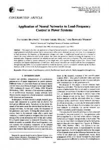
Fig. 1: Block diagram model of hydro-thermal reheat power system

The term „invariant‟ means that the system is completely insensitive to parametric uncertainty and external disturbances [12-13].

2. The Investigated Power System The detailed block diagram modeling of two area thermalhydro power system for load frequency control investigated, is shown in figure 1. An extended power system can be divided into a number of load frequency control areas interconnected by means of tie-lines. Without loss of generality one can consider a two- area case connected by single tie- line [11]. The control objectives are as follows: (i) Each control area as for as possible should supply its own load demand and power transfer through tie line should be on mutual agreement. (ii) Both control areas should controllable to the frequency control. In an isolated control area case the incremental power (PG  PD) was accounted for by the rate of increase of stored kinetic energy and increase in area load caused by increase in frequency. Since a tie line transports power in or out of an area, this fact must be accounted for in the incremental power balance equation of each area.

2.1 Modeling of Tie-Line The power transfer equation through tie- line is [11], V1 V2 (1) P  sin(   ) 12

x

1

2

considering area 1 has surplus power and transfers to area 2 P12 = Power transferred from area 1 to 2 through tie line.

P12 

V1 . V2 . Sin( 1 -  2) X1 2

(2)

For small deviation in the angles and the tie line power changes with the amount i.e. small deviation in  1 and  2 changes by  1 and  2 , Power P12 changes to P12 + P12 Therefore, Power transferred from Area 1 to Area 2 as given in [11] is

2 T o  f1 (s)  f 2 (s)  s T0 = Torque produced The above equation can be represented as in Fig. 2 P12 ( s ) 

Fig. 2 : Block Diagram Representation of a Tie -Line Tie-line bias control is used to eliminate steady state error in frequency in tie-line power flow. This states that the each control area must contribute their share to frequency control in addition for taking care of their own net interchange. Let ACE1 = area control error of area 1 ACE2 = Area control error of area 2 In this control, ACE1 and ACE2 are made linear combination of frequency and tie line power error[11]. ACE1 = P12  b1f1 (4) ACE2 = P 21 b2f2 (5) where the constant b1 & b2 are called area frequency bias of area 1 and area 2 respectively. Now PR1 and PR 2 are mode integral of ACE1 and ACE2 respectively. t (6)

PR1  - Ki1  (P12  b1f 1)dt 0 t

PR 2  - Ki2  (P21  b 2 f 2)dt Where 1 and  2 = Power angles of end voltages V1 and V2 of equivalent machine of the two areas respectively. X12 = reactance of tie line. The order of the subscripts indicates that the tie line power is define positive in direction 1 to 2.

(3)

(7)

0

Taking Laplace transform of the above equation We get

PR1( s )  -

Ki1 P12( s)  b1f1(s)  s

PR 2( s )  -

Ki2 P 21( s)  b2f2(s)  s

(8) (9)

International Journal of Computer Science & Emerging Technologies (E-ISSN: 2044-6004) Volume 1, Issue 4, December 2010

The step changes PD1 and PD 2 are applied simultaneously in control area 1 and 2 respectively. When steady state conditions are reached, the output signals of all integrating blocks will be constant and their input signal must become zero. i.e. P12  b1 f1  0 (input of integrating block - Ki1 ) (10) s

P21  b2 f2  0 ( input of integrating block -

Ki 2 ) ( 11) s

f1 - f2  0 (input of integrating block - 2T 12 ) s

P12 = Ptie,1

and

P21 = Ptie, 2

Therefore Ptie,1  - T12  - 1  constant Ptie, 2 T21 a2 Hence

( 12)

(13)

Ptie,1 = Ptie, 2 = 0

379

of uncertainty happens to arise because of imprecision, ambiguity, or vagueness, then the variable is probably fuzzy and can be represented by a membership function. Defuzzification is the conversion of a fuzzy quantity to a crisp quantity, just as fuzzification is the conversion of a precise quantity to a fuzzy quantity [14]. The out put of a fuzzy process can be the logical union of two or more fuzzy membership functions defined on the universe of discourse of the output variables. There are many methods of defuzzification, out of which smallest of maximum method is applied in making fuzzy inference system [14]. SOM ( SMALLEST OF MAXIMUM) METHOD: This is also called first (or last of maximum) and this method uses the overall output or union of all individual output fuzzy sets Ck to determine the smallest value of the domain with maximum z membership degree in Ck [14]. The equation for *

PR1  PR 2 , And f1  f2  0 Thus, under steady condition change in the tie- line power and frequency of each area is zero. This has been achieved by integration of ACEs in the feedback loops of each area [11]. Control methodology used (PI, FLC & ANN) is mentioned in next preceding sections.

3. Conventional Integral Control When an integral controller is added to each area of the uncontrolled plant in forward path the steady state error in the frequency becomes zero. The task of load frequency controller is to generate a control signal u that maintains system frequency and tie-line interchange power at predetermined values [11]. The block diagram of PI controller is shown in Fig. 3. Where (14)

Fig. 3 : Conventional PI Controller Taking the derivative of above equation (15)

4. Fuzzy Logic Control Fuzzy logic is a thinking process or problem-solving control methodology incorporated in control system engineering, to control systems when inputs are either imprecise or the mathematical models are not present at all. Fuzzy logic can process a reasonable number of inputs but the system complexity increases with the increase in the number of inputs and outputs, therefore distributed processors would probably be easier to implement. Fuzzification is process of making a crisp quantity into the fuzzy [14]. They carry considerable uncertainty. If the form

Z

are as follows:

*

z  inf

zz

z  z  ck ( z )  hgt (ck )}

(16)

The Fuzzy logic control consists of three main stages, namely the fuzzification interface, the inference rules engine and the defuzzification interface [15]. For Load Frequency Control the process operator is assumed to respond to respond to variables error (e) and change of error (ce). e  f

ne

ce

Fig. 4

1/

Z

Basic Fuzzy Logic Controller

nu

nce

Block diagram of a Fuzzy Logic controller

The variable error is equal to the real power system frequency deviation ( f ). The frequency deviation f , is the difference between the nominal or scheduled power system frequency (fN) and the real power system frequency (f). Taking the scaling gains into account, the global function of the FLC output signal can be written as. r (17) Pc  F[nc e(k), nce ce(k)] Where ne and nce are the error and the change of error scaling gains, respectively, and F is a fuzzy nonlinear function. FLC is dependant to its inputs scaling gains [15]. The block diagram of FLC is shown in Fig 4,. nu is output control gain[6]. A label set corresponding to linguistic variables of the input control signals, e(k) and ce(k), with a sampling time of 0.01 sec is as follows: L(e, ce) = { NB, NM, ZE, PM, PB}, Where, NB = Negative Big, NM = Negative Medium, ZE = Zero, PM = Positive Medium, PB = Positive Big Fuzzy logic controller has been used in hydro-thermal interconnected areas. Attempt has been made to examine with five number of triangular membership function (MFs) which provides better dynamic response with the range on input( error in frequency deviation and change in frequency deviation) i.e universe of discourse is -0.25 to 0.25. The numbers of rules are 25.

International Journal of Computer Science & Emerging Technologies (E-ISSN: 2044-6004) Volume 1, Issue 4, December 2010

380

The membership functions (MFs) for the input variables are shown in Fig.5. NB

NM

ZE

PM

PB

Fig. 7 : Multi input neuron model

-0.25 -0.125 0 0.125 0.25 Fig.5 : Membership Function for the control input variables

(20) This expression can be written in matrix form: (21)

Table. 1: Fuzzy inference rule for Fuzzy Logic Controller Input

ce(k)

e(k) NB

NM

ZE

PM

PB

NB

NB

NB

NM

NM

ZE

NM

NB

NB

NM

ZE

ZE

ZE

NM

NM

ZE

PM

PM

PM

ZE

PM

PM

PB

PB

PB

ZE

ZE

PM

PB

PB

5. Artificial Neural Network (ANN) Controller ANN is information processing system, in this system the element called as neurons process the information. The signals are transmitted by means of connecting links. The links process an associated weight, which is multiplied along with the incoming signal (net input) for any typical neural net. The output signal is obtained by applying activations to the net input. The field of neural networks covers a very broad area. Neural network architecture-the multilayer perceptron as unknown function are shown in Fig 6, which is to be approximated. Parameters of the network are adjusted so that it produces the same response as the unknown function, if the same input is applied to both systems. The unknown function could also represent the inverse of a system being controlled, in this case the neural network can be used to implement the controller [17].

Fig. 6: Neural Network as Function Approximator A neuron has more than one input. A neuron with inputs is shown in Fig. 7. The individual inputs p1, p2,…. pR are each weighted by corresponding elements w1,1 , w1,2 ,…w1,R of the weight matrix W. The neuron has a bias b, which is summed with the weighted inputs to form the net input n.

Where the matrix W for the single neuron case has only one row. Now the neuron output can be written as (22) One of the most commonly used functions is the log-sigmoid transfer function, which is shown in Figure 8.

Fig. 8: Log-Sigmoid Transfer Function This transfer function takes the input (which may have any value between plus and minus infinity) and squashes the output into the range 0 to 1, according to the expression: (23) The log-sigmoid transfer function is commonly used in multilayer networks that are trained using the back propagation algorithm, in part because this function is differentiable.

5.1 NARMA-L2 Control The ANN controller architecture employed here is a Non linear Auto Regressive Model reference Adoptive Controller. This controller requires the least computation of the three architectures. This controller is simply a rearrangement of the neural network plant model, which is trained offline, in batch form. It consists of reference, plant out put and control signal. The controller is adaptively trained to force the plant output to track a reference model output. The model network is used to predict the effect of controller changes on plant output, which allows the updating of controller parameters. In the study, the frequency deviations, tie-line power deviation and load perturbation of the area are chosen as the neural network controller inputs.

International Journal of Computer Science & Emerging Technologies (E-ISSN: 2044-6004) Volume 1, Issue 4, December 2010

381

Fig. 9: Simulink Model of two area interconnected hydro-thermal reheat plant with Fuzzy controller

Fig. 10: Simulink Model of two area interconnected Hydro-Thermal Reheat plant with Neural Network controller

Fig. 11: Simulink Model of two area interconnected Hydro-Thermal Reheat plant with PI controller The outputs of the neural network are the control signals, which are applied to the governors in the area. The data required for the ANN controller training is obtained from the designing the Reference Model Neural Network and applying to the power system with step response load disturbance. After a series of trial and error and modifications, the ANN architecture provides the best performance. It is a three-layer perceptron with five inputs, 13 neurons in the hidden layer, and one output in the ANN controller. Also, in the ANN Plant model, it is a three-layer

perceptron with four inputs, 10 neurons in the hidden layer, and one output. The activation function of the networks neurons is trainlm function.300 training sample has been taken to train 300 no of epochs. The proposed network has been trained by using the learning performance. Learning algorithms causes the adjustment of the weights so that the controlled system gives the desired response.

International Journal of Computer Science & Emerging Technologies (E-ISSN: 2044-6004) Volume 1, Issue 4, December 2010

6.

382

Simulation and Results

In this presented work, the hydro-thermal interconnected power system have been developed with PI, fuzzy logic and ANN controllers to illustrate the performance of load frequency control using MATLAB/SIMULINK package. The parameters used for simulation are given in appendix [12]. Three types of simulink models are developed with fuzzy , ANN and PI controller based as shown in Fig. 9 -11 respectively to obtain better dynamic behavior. Refer to Simulink models, frequency deviation plots for thermal and hydro both cases are drawn combined and separately for 1% step load change in system frequency and tie-line power as shown in Fig. 12-20 respectively.

Δf (hz)

Δ P tie (mw)

time(sec) Fig. 15 Change in Tie-line power (hydo-theraml plant) with fuzzy control (Δ P tie)

Δf (hz)

Time(sec) Fig.12 Response of Hydo-thermal plant with fuzzy controller

Time(sec)

Fig. 16 Change in frequency (Hydro plant) with ANN controller (Δf1)

Δf2 (hz)

Δf1 (hz)

Time(sec)

Fig. 13 Change in frequency (thermal plant) –Fuzzy controller (Δf1)

Time (sec)

Fig.17 Change in frequency (Thermal plant) with ANN controller (Δf2)

ΔP tie (mw)

f2 (hz)

Time(sec) Fig. 14 Change in frequency (Hydro plant)- Fuzzy controller (Δf2)

Time (sec) Fig. 18 Change in Tie-line power (hydo-theraml plant) with ANN controller (ΔP tie)

International Journal of Computer Science & Emerging Technologies (E-ISSN: 2044-6004) Volume 1, Issue 4, December 2010

383

Table: 3. Comparative study of peak overshoot Δf1

Δf2

ΔP tie

Area 1 in pu

Area 2 in pu

in pu

PI

0.072

0.072

0.0081

Fuzzy

0.071

0.075

0.0035

0.045

0.055

0.003

Controllers

Δf2 (hz)

ANN

Time (sec)

Fig. 19: Change in frequency (hydro-thermal plant) with PI Controller (Δf)

From the above table it is clear that responses obtained, reveals that ANN controller with sliding gain provides better settling performance than Fuzzy & PI. Therefore, the intelligent control approach using ANN & fuzzy concept is more accurate and faster than the conventional PI control scheme even for complex dynamical system. 8.

ΔP tie (mw)

Time (sec)

Fig. 20 Change in Tie-line power (hydo-theraml plant) with PI controller (ΔP tie) With 1% step load change in both Hydro-Thermal Reheat areas with fuzzy, ANN and PI controllers, the steady state error is minimized to zero. Settling time and maximum peak overshoot in transient condition for both change in system frequency and change in tie-line power are given in table 2 & 3 respectively.

7. Conclusion With 1% load variation in power system the following results are obtained. The Intelligent control approach (Fuzzy Controller and ANN controller) with inclusion of slider gain provides better dynamic performance and reduces the oscillation of the frequency deviation and the tie line power flow in each area in hydro-thermal combination. Table: 2. Comparative study of settling time

Controllers PI Fuzzy ANN

Δf1

Δf2

Area 1

Area 2

(sec)

(sec)

(sec)

105

105

202

23

23

27

17

17

23

ΔP tie

References

[1] George Gross and Jeong Woo Lee, “Analysis of Load Frequency Control Performance Assessment Criteria”, IEEE transaction on Power System Vol. 16 No, 3 Aug 2001 [2] D. P. Kothari , Nagrath “ Modern Power System Analysis”; Tata Mc Gro Hill, Third Edition. [3] Kundur P, “ Power System Stability and Control”, Mc Graw hill New York, 1994. [4] CL Wadhawa “ Electric Power System” New Age International Pub. Edition 2007. [5] Elgerd O. I. , “ Elctric Energy System Theory; An Introduction “ Mc Gro Hill. [6] Jawad Talaq and Fadel Al- Basri , “ Adaptive Fuzzy gain scheduling for Load Frequency Control”, IEEE Transaction on Power System, Vol. 14. No. 1. Feb 1999. [7] P. Aravindan and M.Y. Sanavullah, “Fuzzy Logic Based Automatic Load Frequency Control of Two Area Power System With GRC” International Journal of Computational Intelligence Research, Volume 5, Number 1 (2009), pp. 37– 44 [8] J. Nanda, J.S Kakkarum, “Automatic Generation Control with Fuzzy logic controllers considering generation constraints”, in Proceeding og 6th Int Conf on Advances in Power System Control Operation and managements” Hong Kong , Nov, 2003. [9] A. Magla , J Nanda, “ Automatic Generation Control of an Interconnected hydro- Thermal System Using Conventional Integral and Fuzzy logic Control”, in Proc. IEEE Electric Utility Deregulation, Restructuring and Power Technologies, Apr 2004. [10] A. Demiroren, H.L. Zeynelgil, N.S. SengorThe pplication of ANN Technique toLoad-frequency ControlFor Three-rea Power System” Paper acceptcd for presentation at PPT 001,2001 IEEE Porto Power Tech ConferenceIOth 13'h Septcrnber, Porto, Portugal. [11] Surya Prakash , SK Sinha, “Impact of slider gain on Load Frequency Control using Fuzzy Logic Controller” ARPN journal of Engineering and Applied Science, Vol 4, No 7, Sep 2009. [12] John Y, Hung, “ Variable Structure Control: A Survey”, IEEE Transaction on Industrial Electronics, Vol. 40, No.1 Feb 1993.

International Journal of Computer Science & Emerging Technologies (E-ISSN: 2044-6004) Volume 1, Issue 4, December 2010

[13] Ashok Kumar, O.P. Malik., G.S. Hope. “Variablestructure-system control applied to AGC of an interconnected power System” I.E.E.E. 1EE PROCEEDINGS, Vol. 132, Pt. C, No. 1, JANUARY 1985 [14] Timothy. J. Ross ; „Fuzzy logic with engineering application‟, Mc Gro Hill, International Edition 1995 [15] Q. P. Ha, “ A Fuzzy sliding mode controller for Power System Load Frequency Control”,1998 Second International Conference of Knowledge based Intelligent Electronic System, 21-23 Apr 1998, Adelaide, Australia, [16] M. Masiala,, M. Ghnbi and A. Kaddouri “An Adaptive Fuzzy Controller Gain Scheduling For Power System LoadFrequency Control” 2004 lEEE International Conference on Industrial Technology (ICIT). [17] S Hykin “ Neural Network „ Mac Miller NY 1994. [18] J N Mines‟ MATLAB Supliment to Fuzzy & Neural approach in Engineering‟ John Wiley NY 1997.

Appendix

PDi

Pgi

384

: Incremental load change : Incremental generation change

Author Biographies Surya Prakash Allahabad, 01.05.1971, Received his Bachelor of Engineering degree from The Institution of Engineers(India) in 2003, He obtained his M.Tech. in Electrical Engg. .(Power System) from KNIT, Sultanpur.UP-India in 2009. Presently he is Pursuing Ph. D in Electrical Engg. Load Frequency Control and working as Assistant Professor in SSET, SHIATS(Formerly Allahabad Agriculture Institute, Allahabad- India). His field of interest is Intelligent Control & Power System operation and Control. e-mail: [email protected] [email protected]

MB

09956722055

Dr. S. K. Sinha belongs to Varanasi

Parameters Parameters are as follows: f = 50 Hz, R1 =R2= 2.4 Hz/ per unit MW, Tg = 0.08 sec, Tp=20 sec P tie, max = 200 MW Tr = 10 sec kr = 0.5, H1 =H2 = 5 sec Pr1 = Pr2 =2000MW Tt = 0.3 sec Kp1=Kp2 = 120 Hz.p.u/MW Kd =4.0 ki = 5.0 Tw = 1.0 sec D1 =D2= 8.33 * 10-3 p.u MW/Hz. F : Nominal system frequency Pri : Area rated power, Hi: Inertia constant

Nomenclature Kj : Integral gain Kd, Kp, Ki : Electric governor derivative, proportional and integral gains, respectively. Tw : Water starting time, ACE : Area control error P: Power, E :Generated voltage V: Terminal voltage,  : Angle of the Voltage V Tt : Steam turbine time constant Ri : Governor speed regulation parameter Bi: Frequency bias constant Tpi : 2Hi / f * Di, Kpi: 1/ Di T12 : Synchronizing coefficient, Tg: Steam governor time constant Kr : Reheat constant, Tr : Reheat time constant  : Change in angle, P :Change in power f : Change in supply frequency Di 

PDi fi

R: Speed regulation of the governor KH : Gain of speed governor TH :Time constant of speed governor K1, K2, K3, K4, K5 : Constants Kp : 1/B= Power system gain Tp: 2H / B f0 = Power system time constant

and his date of birth is 17 th Apr 1962. He received the B.Sc. Engg degree in Electrical from R.I.T. Jamshedpur, Jharkhand, India, in 1984, the M. Tech. degree in Electrical Engineering from Institute of Technology, B.H.U, Varanasi, India in 1987, and the Ph.D. degree from IIT, Roorkee, India, in 1997. Currently he is working as Professor & Head, Department of Electrical Engineering, Kamla Nehru Institute of Technology, Sultanpur, UP, India . His fields of interest includes estimation, fuzzy control, robotics, and AI applications. e-mail: [email protected] MB