Artificial Neural Network based Mobile Robot Navigation István Engedy
Gábor Horváth
Budapest University of Technology and Economics, Department of Measurement and Information Systems, Magyar tudósok körútja 2. H-1117, Budapest, Hungary Email:
[email protected]
Budapest University of Technology and Economics, Department of Measurement and Information Systems, Magyar tudósok körútja 2. H-1117, Budapest, Hungary Email:
[email protected]
Abstract—This paper describes a dynamic artificial neural network based mobile robot motion and path planning system. The method is able to navigate a robot car on flat surface among static and moving obstacles, from any starting point to any endpoint. The motion controlling ANN is trained online with an extended backpropagation through time algorithm, which uses potential fields for obstacle avoidance. The paths of the moving obstacles are predicted with other ANNs for better obstacle avoidance. The method is presented through the realization of the navigation system of a mobile robot.
I. INTRODUCTION The field of mobile robotics is a developing industry nowadays. There are numerous appliances of mobile robots. They are sortable based on their operation environment: there are land, aerial, water and underwater mobile robots. They can differ in the level of autonomy they have during operation. Some mobile robots need no human interaction or supervision even in unknown environments, while others are only able to follow a previously painted line on the ground. and there are remote controlled robots, which always need human supervision. In the sequel, we narrow the scope of this paper to the discourse of an autonomous land mobile robot, which is able to navigate in the specified environment. The navigation system of a mobile robot must handle numerous well separable subtasks for right operation. One of these tasks is the localization of the robot and the objects in the surrounding environment. When the whole work area is needed to be known, we are talking about mapping. Another important task is the motion planning. It is divided into at least two separate parts, the path planning, to get the path from one point to another one, and the movement itself, to follow the path. The latter is found to be difficult due to the kinematic constraints of the robot [1]. The path planning is the procedure, which plans the path from the current location to the end point, of which the robot will have to go through. Obviously, the map of the intermediate area is needed to be known, so the obstacles and unreachable areas could be avoided. The area, in which the robot must operate, is continuous; its range could be represented with real numbers, however most algorithms of path planning work only on finite graphs. These algorithms
are for example the well-known Dijkstra, Bellman-Ford, or A* algorithms [2]. The discretization of the area is needed for these graph-based algorithms to be used in path planning. There are many methods for that, like cell decomposition, skeletonization using Voronoi diagram, or making probabilistic road-map [3]. The planning of the path, and going through it are two different things. Not only because the motion could be very complex, but because the movement of the robot must meet various physical constraints, like the momentum of the car, the slip of the wheels, or the minimum turning arch. There are many different ways to keep the robot on its path. The most common solution is to use various controllers, such as P, PD or PID controllers. These provide the system input in real-time, by looping back the measured system output, which is the robot location. The disadvantage of this is that there is a need for a precise model of the system, the robot and the environment in which the robot moves. The motion planning could be carried out in other ways too. Using soft computing methods for motion planning, the path planning and the movement may also be carried out simultaneously. These solutions are becoming more and more popular for robot navigation problems [4]. The soft computing based navigation methods usually utilize fuzzy logic controllers, artificial neural networks, and reinforcement learning methods. They do not require an exact mathematical description of the problem, and therefore they are able to operate in a broader scale. Due to their abstraction skills, they better tolerate the noisy input data. In addition, these solutions may be able to easily adapt to changing circumstances as well. In most of these solutions, the soft computing plays the controller role: in each iteration it decides which direction the car may turn in front of the obstacle, and it provides the needed system inputs, for example the voltage of the motors. Thus, such procedures make mainly local decisions. There is a significant disadvantage of the local decision making. In maze-like situations the robot could go wrong easily, and it is unlikely that it gets to the target. By knowing an exact model of the robot, it can be simulated to see, what path it would take, thus the controlling could be changed accordingly. Backpropagation through time (BPTT) is such
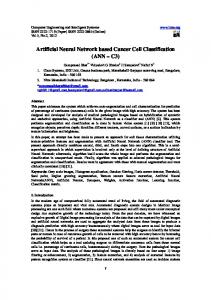
a method [5] that uses this kind of simulation for the improvement of an artificial neural network based controller. However this solution by itself has some disadvantages. It can’t avoid obstacles, because its only goal is to get to the target, and it must use a precise model of the robot for the simulation, otherwise the robot would get far from its target, as the errors accumulate through the simulation. In the sequel we will present a mobile robot navigation solution based on the BPTT method, which could avoid moving obstacles, and needs no precise model of the robot. We also present the realized navigation system in operation in a real car-like robot. II. NAVIGATION METHOD The backpropagation through time method [6] is a training method of dynamic feedback artificial neural networks (ANN) [7]. The main idea of the method is to train the ANN with the usual backpropagation algorithm by opening the feedback loop: the feedback neural network is unfolded through many iteration steps. This way we get a chain of the same ANNs. The training is done in the following way: the input is given to the first ANN, which calculates its own output. This output would be the input of the second ANN, and so on. We get the output of the chain at the output of the last ANN. This output is used to calculate the error, which is then propagated back through the entire chain using the chain-rule. After calculating the partial derivative of the error with respect to each weight, the weights can be modified for example with the Delta-rule, but only in the original ANN, which has been copied many times all along the chain, because of opening the loop. A. The BPTT method in robot navigation The BPTT could be used for robot navigation, as D. Nguyen and B. Widrow showed it [5], “Fig. 1,” where the controller of the robot is an artificial neural network and the whole control loop is opened, including a model of the controlled system.
Fig. 1. BPTT in use of training in a control loop
In this situation not only ANNs take place in the chain, but numerous models of the system, which are not needed to be trained, but the error must be propagated back through them. The models can be constructed using different
approaches: e. g a mathematical model can be used, or the model itself can be constructed by training a properly selected neural network. The former approach is useful if a quite accurate mathematical model can be constructed rather easily, while the latter if the motion equations of the mobile robot are rather complex. In [5] the model was also constructed using a neural network, while in this work the use of a mathematical model was more practical. The input of the model is the output of the controller, which is the control signal, for example the voltage of the motors. The output of the model is the input of the controller, which is the position of the robot. In this case the target position of the robot and the output of the chain are used to calculate the error, which is then propagated back. It could be easily seen that the backpropagation through time is not capable by itself to work with obstacles. The only aspect of the training is to get to the target position at the end of the chain. B. The extension of the BPTT method To make the BPTT method able to take account of the obstacles, we have elaborated the following solution. Based on the location and the size of the obstacles, a potential function can be defined (1), which can be used to repel the robot away from the obstacles. To actually repel the robot, this function must be used to extend the cost function of the Delta-rule. The cost function is regularized with the potential field (3), so the goal of the weight modification is not only to minimize the error at the end of the simulation chain, but also to minimize the potential of the path, to get the robot the farthest from the obstacles. This way the obstacles could be avoided. , , otherwise
(1) (2)
,
∑
(3)
∑ th
is the potential function of the i obstacle (1). is the distance of the robot from the center of the ith obstacle (2), and is the radius of the ith obstacle. The parameter ε is a finite positive real number; it ensures the value of the potential field to be always finite. In (2) and are the coordinates of the location of the obstacle, and and are the coordinates of the position of the car. , is the regularized cost function (3). Its first term is the usual squared deviation of the simulated end position ( ) from the target position ( ). This term is responsible to get the robot to the target at the end of the simulation. The end position is the output of the simulation chain, so it is the position of the robot at the end of the simulation. Only this robot position is used to calculate the error for the weight modification of the ANNs. The second term of the cost function is the regularization term. It is responsible for the obstacle avoidance. It uses each ANNs’ outputs, each robot positions along the simulation chain to calculate the
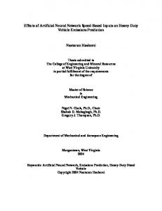
potential of each obstacle, because the collision must be avoided all along the path, not just at the last step. This is why the potential field is summarized through i. The summarizing through j refers to the superposition of the potential field of multiple obstacles. This cost function is minimized with the weight modifying algorithm of the neural network. In this case we use the backpropagation algorithm to do so. The partial derivative of the cost function with respect to each weight / is needed, which can be expressed by the chain-rule as the product of the partial derivative of the cost function with respect to the actual robot position / , and the partial derivative of the actual robot position with respect to each weights / (4). (4) The first term of the cost function, the squared deviation of the end position from the target, is propagated back in an ANN the same way as it was described in the disclosure of the BPTT method, so the regularization term could be added to the error during the backpropagation at the appropriate places through the simulation chain, and the weights of the ANN can be modified using the usual way as it can be seen in Fig. 2.
Fig. 2. Adding the obstacle potential to the error
The backpropagated error, which has the same dimension as the state of the robot, contains four values, the two coordinates of the location, and two coordinates of the orientation of the robot. The orientation is described with the two coordinates of a two dimensional vector. The orientation is the angle of this vector. This way the angle can be described with continuous functions, which are needed by the ANN. However the potential function depends only on the location of the robot, so the derivative of the potential field with respect to the orientation is zero. The partial derivative of the potential field with respect to the location of the robot is a gradient vector (5). The gradient vector points out of the center of the obstacle. It is not necessary to calculate the value of the potential field, since it is not used anywhere, only the gradient vector must be known in each simulation step. The calculated error from the gradient vector is simply added to the backpropagated error at the appropriate places. . .
2
;
,
2
;
, otherwise
(5)
C. Moving obstacle avoidance by online training With this extension of the BPTT algorithm predefined static obstacles can be avoided. To use this method to navigate among moving or previously unknown obstacles, further modifications must be made. Till this point, we did not specify, whether the ANN is to be trained offline or online, i.e. whether it was trained before the actual usage or during it. Offline training could be used, if the obstacles were previously known and static. In such cases the training could be carried out from multiple starting points to the only target, so no matter where the robot is at start, it can navigate to the target. In case of moving, or previously unknown obstacles, it is worth considering using online training despite its trivial drawback: the increased need of computational power. Online training, that is when the training of the ANN and the use of it are happening at the same time, brings the ability to adapt to changing environment, e.g. to moving or previously unknown obstacles. It has also many advantages. There is no need for training the ANN from multiple starting points, only the current location of the robot should be used, because the robot is at that location, not in any other. This makes the training much faster. Using the online training makes the method to an anytime algorithm, because the navigation result is degraded only in quality with the decreasing computing power or time limit. This makes the algorithm well-scalable; it works even on a slower CPU, but using a faster one is only increasing the quality of the result of the algorithm. To avoid the moving obstacles, the newest obstacle positions must be used in all training iteration steps. This way the robot can avoid moving obstacles that are moving slower than the robot. This method takes into count only those obstacles that are close to the robot or its planned path. So the robot only ‘notices’ the obstacles, when they are directly in the way of the robot. If these obstacles change their location faster than the robot could, they can even hit the robot, so this way the collision might be unavoidable. If the obstacles move slower than the robot, the robot has time to eventually avoid them. This solution has a drawback: all those obstacles, which are not close to the path, but moving towards it, are not taken into consideration, but their trajectory and even the position of the collision could be predicted. D. Fast-obstacle avoidance by position prediction To make the navigation method able to avoid obstacles that move faster than the robot, the prospective positions of the obstacles must be known. This is only possible by prediction. There are many ways to predict the future positions of the obstacles, but all of them needs that we know some of the previous samples of the position-time function of the obstacle. This problem can be taken as an extrapolation problem, so most of these methods are known extrapolation methods. The easiest way is to use the sample
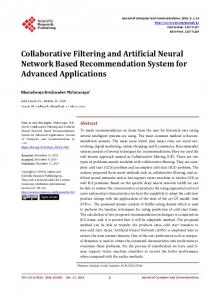
points to fit a polynomial onto them. This way the future positions could be extrapolated. There are also soft computing methods to predict a time series. To predict the prospective positions of the obstacles, we use also dynamic ANNs, which are trained with the previous positions of the obstacles. One training point consists of a target point, which is one point of the time series, and some input points, which are the previous points in the time series, in the proper order. The training of the ANN is done the usual way, using the backpropagation algorithm. Time series prediction is considered as a modeling task when a dynamic neural network is used to model the system generating the time series, in this case, the obstacles and all their physical constraints. The complexity of the system determines how many previous sample points should be used in the input of the ANN. Also the sampling rate is determined by the system too. In this case the sampling rate was predetermined by the hardware elements, as it will be described in section III. The complexity of the movement of an obstacle is a harder question to answer. If we narrow the scope of obstacles only to passive objects, which does not have any logic or intelligence and move only by their inertia, the complexity of their movement would be low. If we assume that the obstacles could have some inner intelligence, the prediction could be even impossible, because the obstacle might decide to alter its route. Therefore we did not want to predict all possible obstacles. We have elaborated a method that is able to predict the movement of objects similar in its moving pattern as the robot. This makes possible to use this method in collaboration environments, like robot soccer. Because there might be more obstacles, one ANN is allocated to each obstacle. The ANN is trained with the usual training samples, inputs and target. The inputs are some of the previous positions in order, and the target is the following position in the path of the obstacle. This can be seen on Fig. 3. in three steps, lines marked with different styles.
Fig. 3. The obstacle position predicting ANN
At the beginning of the navigation, there are insufficient samples, so more samples are needed to be collected, before the robot can start moving. Another problem is that when
there are just enough samples, they make too few training point, to train an ANN. In such situation it is better to use fewer samples in the input of the ANN, and make more training points, and as more samples are collected, the length of the input of the ANN could be increased. The predicted obstacle positions can be used as an input to predict more positions, so the prospective path of the obstacle can be predicted. This predicted path is used in the potential field calculation, calculating always with the proper obstacle position, according to the moment of the given simulation step. This method makes it possible to avoid collision with obstacles in the future that are not close to the path of the robot at the beginning of the navigation, but they are moving towards the robot. III. NAVIGATION SYSTEM The navigation method described in the previous section is utilized in a complete navigation system, which can control both a simulated and a real wheeled robot. This described navigation method is the motion planning part of the system. A complete navigation system however needs localization too. The localization of the robot and the obstacles is made through observing the work area, using a camera, which is attached to the ceiling above the area, where the robot is moving. Every camera frame is processed by an image processing algorithm, which is able to determine the positions and the orientations of the robot, the target, and the obstacles, based on the markers, placed on them. The algorithm used to do this is beyond of the scope of this paper, so it is not presented here. With the localization of the robot on every camera frame, the control of the robot has become a closed loop control. This makes it possible that if the model of the robot and the real physical robot differs, that is if the model describes only approximately the moving system, the closed loop control can still navigate the robot well. A brief summary of the main components and their relations in the navigation system is shown on Fig 4, where this closed loop can be noticed easily. The software doing the control is running on a PC, which has the camera attached to it. The PC is connected to the real robot through so-called gateway hardware, using a radio link with a protocol, which has basic commands like setting the speed of the wheels of the robot, or stop both wheels.
Fig. 4. The operation of the navigation system
The controlled wheeled robot is shown on Fig 5. It is called ‘MITMÓT robot’, and it was designed and developed at the Department of Measurement and Information Systems at Budapest University of Technology and Economics [8]. As it can be seen, it has two independently driven wheels, and one steady wheel. It can turn the wheels in both direction, but during the tests of the navigation system, we decided to use the robot only in forward mode, to force it to make turns instead of turning towards the target right at the start. The robot is pretty slow; its maximum speed is about 15 cm/sec.
shown how this can be inserted into a navigation system with localization. The following images have been taken by the application. Fig. 6. shows two cases of static obstacle avoidance with one and two obstacles. Fig. 7. shows a case of moving obstacle avoidance. The small circles are the predicted prospective positions (green); and the previous positions (red). These images are just samples, how this navigation system can perform. There are of course situations, where the navigation method does not find the shortest route, or the route has some unnecessary loops. The online training of the network needs serious computation power. However, it can perform well on a middle-class CPU in 2009; it does not collide with the obstacles, and gets to the target. V. CONCLUSIONS In this paper we have shown that the classical BPTT training approach can be extended using regularization, where through the regularization term additional constraint can be taken into consideration. Here the constraints came from the need of avoiding static or moving obstacles in a navigation problem. It was also shown that real time online training is possible if the speed of the moving objects – the mobile robot and the obstacles – is rather small. For similar problems with higher speed the speed of computing should also be increased that can be achieved e.g. using hardware acceleration such as graphical processors. VI. REFERENCES [1] [2] [3] [4]
Fig. 5. The controlled wheeled robot, called MITMÓT robot
IV. RESULTS We have presented an ANN-based robot navigation system, which is capable to evade moving obstacles using a regularized version of the BPTT method. We have shown how the regularization could be carried out with a potential field, and how this is used for obstacle evasion. We have presented a solution to avoid fast-moving obstacles as well, predicting the future route of the obstacles. We have also
[5] [6] [7]
[8]
J.-C. Latombe, Robot Motion Planning. Boston , MA : Kluwer, 1991. Stuart Russel, Peter Norwig: Artificial Intelligence A Modern Approach , Prentice Hall 2003 Sebastian Thrun, Wolfram Burgard, Dieter Fox: Probabilistic Robotics, MIT Press 2005 Pratihar, D.K.: Algorithmic and soft computing approaches to robot motion planning. Mach. Intell. Robot Control 5,1-16 (2003) D. Nguyen and B. Widrow, ``The Truck Backer-Upper: An Example of Self-Learning in Neural Networks,'' Proceedings of the International Joint Conference on Neural Networks, 2:357-362, 1989. M. Minsky and S. Papert. Perceptrons: An Introduction to Computational Geometry. The MIT Press, Cambridge, Massachusetts, 1969. D. E. Rumelhart, G. E. Hinton, and R. J. Williams. Learning internal representations by error propagation. In D. E. Rumelhart and J. L. McClelland, editors, Parallel Distributed Processing: Explorations in the microstructure of cognition; Vol. 1: Foundations, Cambridge, Massachusetts, 1986. The MIT Press. MITMÓT – http://bri.mit.bme.hu - Department of Measurement and Information Systems at Budapest University of Technology and Economics
Fig. 6. Static obstacle avoidance
Fig. 7. Moving obstacle avoidance