Original Article Folia Primatol 2005;76:303–324 DOI: 10.1159/000089530
Received: July 22, 2004 Accepted after revision: February 23, 2005
Artificial Neural Networks and Three-Dimensional Digital Morphology: A Pilot Study Roger L. King a
A.L. Rosenbergerb
L. Leann Kandac
a
Mississippi State University, Mississippi State, Miss., b Brooklyn College, CUNY, New York, N.Y., and c University of Massachusetts, Amherst, Mass., USA
Key Words Artificial neural networks ` Unsupervised learning ` Laser digitizing ` Three-dimensional digital morphology ` Dentition ` Anthropoids ` Systematics
Abstract In this pilot study, we used an unsupervised learning algorithm for selforganization and pattern matching to create feature maps that can be applied to morphological problems. We designed a network to analyze 83 first and/or second upper and lower molar sets representing 14 anthropoid primate species, based on three-dimensional measures obtained from laser-digitized, virtual specimens. As shown in a comparison with a principal-component analysis of the virtual specimens, the artificial neural network approach provided more biologically meaningful information than the conventional multivariate analysis approach. The methodology discovered partitions and hierarchical clusters consistent with anthropoid systematics, from the species (or subspecies) level to the highest categories, by sorting and allocating upper and lower molar teeth. As one might expect, measures of upper molars were richer in phenetic information than those of lower molars, even among the anatomically diverse platyrrhines. We also show that reducing taxonomic noise (i.e. biological variation) by limiting the analysis to a monophyletic subset improves discrimination. Copyright © 2005 S. Karger AG, Basel
Introduction
In this report, we present a pilot study that applies an artificial neural network (ANN) architecture to a database of three-dimensional (3-D) digital morphology measures describing a diverse sample of anthropoid molar teeth. 3-D digital mor-
Ó2005 S. Karger AG, Basel Fax + 41 61 306 12 34 E-Mail
[email protected] www.karger.com
Accessible online at: www.karger.com/fpr
Roger L. King, Department of Electrical and Computer Engineering, Box 9571, Mississippi State University Mississippi State, MS 39762-9571 (USA) Tel. +1 662 325 2189, Fax +1 662 325 2298 E-Mail
[email protected]
phology, the study of form based upon 3-D digitized or virtual specimens, has many advantages [Ungar and M’Kirera, 2003], both theoretical and practical. The key benefits we exploit here are the potential to define and extract precise measures that are more realistic descriptors of complex anatomical form than caliper measures. Using accurately digitized specimens, one can take linear (point to point), conventional two-dimensional (2-D; compound point to point measures describing a plane) and 3-D measures, i.e. explicit multi-point dimensions of contours, surfaces and volumes which accurately represent structural shape or space, as defined by their geometric coordinates. ANNs are hardware and software implementations based on biological models of circuitry and process used by humans to accomplish many fundamental tasks, such as pattern recognition, memory and visualization. Like the brain, ANNs employ simple processors with a high degree of parallelism. The strength of the ANN architecture used in this study that appeals to comparative morphology and systematics is its potential for knowledge discovery, pattern recognition, adaptability and self-organization. Our pilot study has two goals: (1) to apply the approach of ANNs to a sample of anthropoid molar teeth in order to investigate its potential as a systematics tool and (2) to begin to evaluate the power of geometrically true 3-D measures, as opposed to standard caliper measures, as quantitative descriptors of molar morphology. The samples we have chosen do not reflect any particular systematics or anatomical problem. Rather, they were selected to represent a range of morphologies, a diversity of phylogenetic groups, a mixture of interspecific and intraspecific pairings of interest, and because we had convenient access to the material. ANNs and Unsupervised Learning ANNs are systems of simple processors (neurons) that are interconnected in an organized fashion (architecture). There are numeric values associated with the interconnections (weights) that are adjusted over time to create a mapping between a n-dimensional input space and a m-dimensional output space. These weights represent the knowledge about the problem domain. Changes in the weights are analogous to learning. A specific architecture will have a learning algorithm associated with it, and each of the neurons in the architecture will make use of a function (linear or nonlinear) to describe the neuron’s internal state (activation) resulting from received stimuli. The architectures (neurons and their interconnections) are computational approaches simulating the biological neural network. Therefore, many of the architectures, including the one used in this study, are based on findings from the field of neuroscience [Kohonen, 1989]. Learning in an ANN can occur in either a supervised or an unsupervised fashion. A supervised approach uses a learning algorithm that creates an input/output mapping based on a labeled training set (i.e. an input vector is paired with a correct output vector). In this case, the network will learn a functional approximation from the input/output pairings and will have the ability to recognize or classify a new input vector into a correct output vector (generalization). An unsupervised learning architecture, in contrast, presents the network with only a set of unlabeled input vectors. Unsupervised learning is used for data compression, feature discovery and classification. The sole information available to the network is the correlations it derives from the input vectors. The network is expected to create charac304
Folia Primatol 2005;76:303–324
King/Rosenberger/Kanda
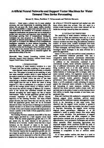
terizations about the input vectors from these correlations and to produce outputs corresponding to a learned characterization (i.e. knowledge discovery) [King, 1998]. As with humans, learning with ANNs takes time. When using either a supervised or an unsupervised learning algorithm, data are presented to the network numerous times. One complete presentation of a set of training data is referred to as an epoch. As the data are repeatedly presented to the network, the learning algorithm evolves the weights connecting the neurons (i.e. learns). It is within the weights that knowledge is stored (represented) about the relationships being learned or discovered by the network. ANNs that use unsupervised learning have the goal of determining natural clusters or feature similarity within the data set and to display its results in a meaningful manner. Since no labeled training sets are used in this approach, the outputs from the unsupervised learning network must be examined by a domain expert to determine if the classification provides any new insight into the data set. If the result is not reasonable, then an adjustment is made to one of the training parameters used to guide the network’s learning, and the network is presented the patterns again. However, before examining the more complex self-organizing map (SOM) architecture, it is beneficial to recall a simpler form of unsupervised learning that makes use of a clustering algorithm. These networks utilize input data in a vector form, and a distance metric (e.g. Hamming distance, Euclidean distance) is used to determine nearness (similarity) of a new input pattern to an existing cluster. Decision options for the network are to include the new pattern into an existing cluster or to create a new cluster for this pattern. Learning (i.e. weight adjustment) normally occurs after a pattern has been assigned to a cluster. In the case of a clustering algorithm, this is simply adjusting the weights defining the center of the cluster. An example of this type of unsupervised learning network is k-means clustering [Moon and Stirling, 2000]. Self-Organizing Maps Kohonen [1989] proposed that there is a general tendency in human information processing to compress complex information by forming reduced representations of the most relevant facts. An important aspect of this reduction in dimensionality is the ability to preserve the structure (interrelationships) of the information. He proposed that this simplified representation is accomplished via spatial ordering of processing units (neurons) within the brain. However, this ordering did not involve movement of any neurons but a change in the internal parameters of identical units. A self-organizing feature map algorithm is used to convert patterns of arbitrary dimensionality into the responses of 2- or 3-D arrays of neurons (maps). A SOM may be thought of as a self-organizing cluster. It is clustering because of its tendency for data compression and it is self-organizing because similar clusters are spatially near on the map. The basic components of a 2-D SOM are shown in figure 1. Note that each element of the input vector x (description of unknown specimen) is connected to each of the processing units on the map through the weight vector wij. After training, the SOM will define a mapping between the input data space and the 2-D map of neurons. The output yi of a processing unit is then a function of the similarity between the input vector and the weight vector. The nonlinear mapping Neural Networks and 3-D Digital Morphology
Folia Primatol 2005;76:303–324
305
Fig. 1. Graphic depiction of data analysis using an ANN and a SOM (see text).
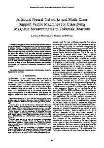
Fig. 2. Rectangular grid used for SOMs showing 4 nearest neighbors.
of the SOM utilizes a technique developed by Sammon [1969] that preserves the higher dimensional nearness on the map. In other words, if two vectors are near each other in high dimensional space, then they are near on the map. Figure 1 shows how a trained feature map would respond with a winning output neuron when excited by an original training pattern or an unknown input vector pattern that is similar. Knowledge about the significance of the area around the winning neuron will then help the user in knowledge discovery. The SOM feature 306
Folia Primatol 2005;76:303–324
King/Rosenberger/Kanda
map also functions as a nonlinear projection of the probability density function of the high dimensional input vector onto the 2-D display [Kohonen et al., 1996]. This means that following the formation of the self-organized internal representation for existing implicit relationships between the 12-D original training data (i.e. after learning), the same implicit input spatial relationships become explicit on the feature map. In simpler terms, if two points are close on the 2-D map, then they were also close in the higher dimensional space. In other words, after training, the internal representation for knowledge about the relationships within the original training data becomes explicit on the feature map. The SOM algorithm is typically implemented on a planar array of neurons (fig. 2) with spatially defined neighborhoods (e.g. hexagonal or rectangular arrays, with 6 or 4 nearest neighborhoods, respectively). Also, the map must contain some method of compressing the data into a manageable form. One important attribute of a SOM is that it performs data compression without information being lost with regard to the relative distance between data vectors. A SOM typically uses the Euclidean distance to determine the relative nearness or similarity of data. The idea of a spatial neighborhood, Nm, is used in measuring the similarity between the input vector and values of the reference vector represented by the vector of weights between the input layer and all of the neurons on the map. Before training begins, the weights are randomized and a learning rate and neighborhood size are selected. Then, when a training vector is presented to the network, it finds the neuron on the map with the most similar weight values. The weights of the winning neuron and the neighborhood neurons are then adjusted (learning) to bring them closer to the training vector. Over the course of the iterative training process, the neighborhood size and learning rate are independently decreased until the map no longer makes significant adjustments. The result is that the neurons within the currently winning neighborhood undergo adaptation at the current learning step while the weights in the other neighborhoods remain unaffected. The winning neighborhood is defined as the one located around the best matching neuron, m. The operation of the SOM algorithm progresses as follows. First, for every neuron i on the map, there is associated a parametric reference vector wi. The initial values of wi (0) are randomly assigned. Next, an input vector x (Rn) is applied simultaneously to all of the neurons. The smallest of the Euclidean distances is used to define the best-matching neuron; however, other distance metrics may be explored to determine their efficacy in clustering the codebook vectors [King et al., 1993]. As the training progresses, the radius of Nm decreases such that Nm(t1) > Nm(t2) > Nm(t3)..., where t1 < t2 < t3... In other words, the neighborhood of influence can be very large when learning begins, but towards the end of learning, the neighborhood may involve only the winning neuron. The SOM algorithm also uses a learning rate that decreases with time. In summary, the self-organization of the map proceeds as follows: (1) the map is presented with a sufficient number of training patterns; (2) weights are only adjusted on the neurons in the winning neighborhood, and (3) the adjustment is in proportion to the activation received by each neuron in the neighborhood. The effect of this weight adjustment rule is a tendency to enhance the same responses to a sufficiently similar subsequent input. As a result, a map is obtained with weights coding the stationary probability density function of the pattern vectors used for the Neural Networks and 3-D Digital Morphology
Folia Primatol 2005;76:303–324
307
training. The map also displays the data from a different viewpoint; instead of viewing the data as a n-dimensional vector, it can be viewed as a 2-D plot. This is where expert human analysis is enhanced. Instead of looking at the n-dimensional input vector of a sample and trying to determine what its meaning is, one need only look at the location of the sample on the map. Materials and Methods Measurements We used a high-resolution laser scanner with an accuracy of 0.025 mm to generate an array of x,y,z coordinate points to describe 83 first and/or second upper and lower molar teeth of 14 anthropoid primate species. Each of the specimens was digitized at a density of approximately 150 points/mm2. This density level faithfully captures surface detail in very small specimens. Using this figure as a standard also means that the amount of surface relief described per unit area is comparable across all cases. This serves to minimize bias in measurements of area and volume, which would be sensitive to the size and shape (topographic) differences present in the sample. Our methodology for collecting coordinate data and the editing process involved in deriving measurements from the data – such as the demarcation of anatomical features for measurement – has been proven in numerous repeat trials [Rosenberger and Kellogg, unpubl. observations]. Negligible error was found in measurement replication tests within and between specimens. Linear measures taken on population samples of virtual specimens were also statistically indistinguishable from typical caliper measurements taken on the actual specimens. The following measurements were used: Laser basal length (LBL): on a digital specimen aligned with the mesiodistal axis parallel to the x-axis, LBL is the distance between minimum and maximum x-coordinate values in the x-axis. Laser basal breadth (LBB): on a digital specimen aligned with the mesiodistal axis parallel to the x-axis, LBB is the distance between minimum and maximum y-coordinate values found anywhere between the occlusal table of the crown and the cervix. Laser basal area: LBL × LBB (mm2). Occlusal table area: area of the occlusal table, or ‘chewing surface’ of upper and lower molars, i.e. the aspect contained within the boundaries of the cusp-crest system and excluding the crown sidewalls, except for the wear facets of the upper lingual notch and lower buccal ectoflexid. Cusp height: height of a cusp tip above the lowest point in the trigon or talonid basin of an upper or lower molar, respectively, in the z-axis. Apical distance: the oblique distance between the apical tip of a cusp and the lowest point in the trigon or talonid basin of an upper or lower molar, respectively. Samples Species comprising the 83 cases used in this study are listed in table 1. The living forms range in weight, approximately, from a 300 g Callithrix penicillata to an 11,000 g Colobus satanus; molar lengths range from 2.3 to 7 mm, respectively, to 10 mm in the fossil catarrhine Oreopithecus bambolii. We digitized sharp epoxy or plaster casts of molars or tooth rows showing little or no detectable wear rather than actual specimens; mounting jaws would have required additional setup time. Except for a few fossils, each individual was represented by an occluding set of teeth. In the extant species, except for callitrichines, an upper and lower second molar set was used. First molars were substituted for the M2s in callitrichines, as the second molars are highly reduced even in the three-molared Callimico. For the fossils, these conditions were relaxed. All have been identified as likely second molars, but uppers and lowers did not necessarily belong to the same individuals. In a few cases, including Oreopithecus, the fossil samples were also moderately worn.
308
Folia Primatol 2005;76:303–324
King/Rosenberger/Kanda
Table 1. Samples and measurements used in this study Taxon
Pat- Hypo- Hypo- Proto- Proto- Meta- Meta- Entotern conid conid conid conid conid conid conid No. Z AD Z AD Z AD Z
Ento- LBL conid AD
LBB LBA
OTA
Colobus satanus Colobus powelli Procolobus verus Macaca nigra Oreopithecus Oreopithecus Oreopithecus ?Prohylobates sp. ?Prohylobates sp. Aotus trivirgatus Aotus trivirgatus Callicebus moloch Callicebus moloch Callicebus moloch Saimiri sciureus Saimiri sciureus Saimiri sciureus Saimiri sciureus Saimiri sciureus Saimiri sciureus Saimiri sciureus Saimiri sciureus Saimiri sciureus Saimiri sciureus Callithrix jacchus Callithrix jacchus Callithrix jacchus Callithrix jacchus Callithrix jacchus Callithrix jacchus Callithrix penicillata Callithrix penicillata Callithrix penicillata Callithrix penicillata Callithrix penicillata Callimico goeldii Callimico goeldii Callimico goeldii Callimico goeldii Callimico goeldii Colobus satanus Colobus brunneus Colobus powelli Procolobus verus Macaca nigra Oreopithecus Oreopithecus Oreopithecus Rangwapithecus ?Prohylobates sp. ?Prohylobates sp. ?Prohylobates sp. Aotus trivirgatus
1 2 3 4 5 6 7 8 9 10 11 12 13 14 15 16 17 18 19 20 21 22 23 24 25 26 27 28 29 30 31 32 33 34 35 36 37 38 39 40 41 42 43 44 45 46 47 48 49 50 51 52 53
3.13 2.28 2.49 3.11 3.49 3.40 3.71 3.08 2.06 1.45 1.70 1.25 1.13 1.08 1.01 1.07 0.90 1.07 1.11 0.95 1.02 1.11 1.09 1.19 0.66 0.73 0.62 0.73 0.74 0.54 0.97 0.89 0.88 0.79 0.86 1.25 1.06 0.96 1.05 1.07 2.77 2.34 2.15 2.59 2.42 3.25 1.56 2.98 2.33 2.41 1.97 2.12 1.28
6.32 4.14 5.04 7.78 7.58 7.75 9.10 6.22 7.12 3.07 3.20 3.09 3.03 3.01 2.66 2.70 2.67 2.63 2.56 2.85 2.60 2.78 2.53 2.66 2.05 2.13 1.99 2.14 2.26 2.05 2.27 2.12 2.19 2.13 2.10 2.46 2.41 2.33 2.39 2.31 7.58 6.81 5.23 5.33 8.99 9.74 9.04 9.63 9.82 8.95 8.45 8.23 3.97
43.51 24.12 31.65 63.49 85.89 65.10 89.95 27.42 55.32 8.99 10.51 10.13 10.88 10.40 6.91 6.39 6.86 6.55 6.44 5.97 6.30 6.04 6.06 6.32 4.06 3.93 4.12 4.30 3.82 4.28 3.99 4.54 4.68 4.46 4.52 6.86 6.27 5.28 5.57 5.95 48.89 45.97 24.72 32.30 57.79 77.73 57.44 69.31 72.67 46.21 34.41 37.14 8.89
1.58 1.31 1.85 1.36 0.19 0.71 –0.03 2.37 1.35 0.57 0.58 0.74 0.79 0.52 0.73 0.69 0.73 0.61 0.84 0.74 0.66 0.75 0.78 0.75 0.50 0.58 0.68 0.81 0.54 0.67 0.64 0.60 0.80 0.62 0.83 0.74 1.05 0.72 0.53 0.92 2.03 0.56 1.36 1.01 1.61 0.81 0.66 0.59 1.40 1.68 1.32 1.75 0.95
3.27 2.40 3.67 2.40 2.53 2.77 2.86 3.03 3.26 1.28 1.18 1.35 1.39 1.27 1.23 1.21 1.14 1.15 1.34 1.28 1.22 1.16 1.33 1.22 1.02 1.03 0.91 0.97 0.82 1.09 1.02 0.83 0.99 0.95 1.09 1.25 1.25 1.12 0.83 1.48 3.27 3.32 2.59 2.30 2.90 3.33 2.72 3.24 5.77 2.89 3.29 2.49 1.45
1.62 1.45 1.84 1.69 0.38 1.41 0.93 1.67 1.82 0.65 0.97 1.27 1.13 0.82 1.03 1.17 1.05 1.13 0.97 0.91 1.04 1.03 1.06 0.92 0.82 0.99 0.93 1.03 0.81 0.96 1.01 0.90 1.05 0.91 1.02 0.92 1.14 0.96 0.84 1.21 2.17 0.64 1.67 1.31 1.91 0.83 0.69 1.06 1.87 1.53 1.22 1.25 1.23
Neural Networks and 3-D Digital Morphology
2.96 2.38 2.99 3.20 3.39 3.83 3.28 2.30 3.75 1.57 2.29 2.54 2.46 2.45 1.62 1.67 1.86 1.69 1.66 1.91 1.78 1.40 1.56 1.37 1.37 1.60 1.44 1.64 1.32 1.53 1.45 1.50 1.41 1.35 1.66 1.66 1.63 1.42 1.39 1.46 3.63 4.06 2.51 3.15 3.86 3.27 2.82 2.96 4.69 2.72 3.33 2.48 1.66
2.92 2.14 2.14 2.75 1.23 1.34 1.81 1.72 2.52 1.23 1.65 1.56 1.18 1.38 1.08 1.17 1.10 1.28 1.23 0.84 1.26 1.22 1.26 1.07 1.00 0.96 0.76 0.84 0.80 0.76 1.06 0.98 1.07 0.99 1.00 0.75 1.14 1.03 1.32 1.27 2.12 2.61 2.08 2.07 1.75 1.48 0.91 0.83 1.56 1.80 1.17 1.34 0.65
3.83 2.47 2.78 4.42 3.22 3.44 3.42 2.88 3.37 1.66 2.46 2.14 1.97 2.17 1.47 1.50 1.61 1.68 1.50 1.34 1.66 1.68 1.60 1.54 1.36 1.34 1.18 1.24 1.31 1.22 1.41 1.33 1.32 1.25 1.39 1.06 1.57 1.34 1.65 1.51 3.17 3.48 2.41 2.42 3.29 4.38 3.16 3.99 3.02 2.87 2.21 2.49 1.57
2.29 1.87 1.70 2.20 0.34 0.40 –0.02 2.10 1.35 0.95 1.01 0.76 0.59 0.82 0.56 0.50 0.62 0.59 0.90 0.54 0.76 0.56 0.68 0.57 0.38 0.48 0.33 0.38 0.28 0.35 0.56 0.48 0.53 0.43 0.49 0.75 0.65 0.42 0.56 0.41 1.99 1.68 1.69 1.36 1.63 0.75 0.37 0.30 1.18 1.57 1.28 1.48 0.57
Folia Primatol 2005;76:303–324
6.75 6.25 5.13 8.37 9.88 9.50 11.12 6.75 8.12 3.50 3.37 3.38 3.62 3.75 2.75 2.61 2.88 2.62 2.63 2.75 2.50 2.63 2.50 2.63 2.12 2.00 2.50 2.25 2.13 2.12 2.25 2.50 2.25 2.13 2.38 3.00 2.62 2.38 2.37 2.62 6.63 6.50 6.12 5.13 8.75 11 8.98 9.37 8.75 7.50 7.00 7.38 3.12
42.66 25.88 25.86 65.12 74.89 73.63 101.19 41.99 57.81 10.75 10.78 10.44 10.97 11.29 7.32 7.05 7.69 6.89 6.73 7.84 6.50 7.31 6.33 7.00 4.35 4.26 4.98 4.82 4.81 4.35 5.11 5.30 4.93 4.54 5.00 7.38 6.31 5.55 5.66 6.05 50.26 44.27 32.01 27.34 78.66 107.14 81.18 90.23 85.93 67.13 59.15 60.74 12.39
309
Table 1 (continued) Taxon
Pattern No.
Hypo- Hypo- Proto- Proto- Meta- Metaconid conid conid conid conid conid Z AD Z AD Z AD
Entoconid Z
Entoconid AD
LBL
LBB
LBA
OTA
Aotus trivirgatus Callicebus moloch Callicebus moloch Callicebus moloch Saimiri sciureus Saimiri sciureus Saimiri sciureus Saimiri sciureus Saimiri sciureus Saimiri sciureus Saimiri sciureus Saimiri sciureus Saimiri sciureus Saimiri sciureus Callithrix jacchus Callithrix jacchus Callithrix jacchus Callithrix jacchus Callithrix jacchus Callithrix jacchus Callithrix penicillata Callithrix penicillata Callithrix penicillata Callithrix penicillata Callithrix penicillata Callimico goeldii Callimico goeldii Callimico goeldii Callimico goeldii Callimico goeldii
54 55 56 57 58 59 60 61 62 63 64 65 66 67 68 69 70 71 72 73 74 75 76 77 78 79 80 81 82 83
0.90 0.92 0.83 0.63 0.67 0.62 0.67 0.70 0.68 0.45 0.62 0.84 0.57 0.65 0.00 0.00 0.00 0.00 0.00 0.00 0.00 0.00 0.00 0.00 0.00 0.00 0.00 0.00 0.00 0.00
1.06 0.86 1.05 0.85 0.58 0.84 0.75 0.59 0.66 0.70 0.54 0.59 0.69 0.61 0.94 0.87 0.68 0.91 0.79 0.74 1.06 0.77 0.89 0.88 0.79 0.87 0.93 0.91 0.61 0.73
1.60 1.35 1.62 1.57 1.15 1.04 1.28 1.06 1.00 1.21 0.94 1.08 1.08 1.33 1.46 1.30 1.01 1.49 1.10 1.32 1.52 1.34 1.52 1.41 1.24 1.31 1.13 1.42 1.11 1.17
3.37 3.37 3.37 3.25 2.63 2.5 2.5 2.38 2.25 2.5 2.5 2.38 2.5 2.5 2.38 2.37 2.12 2.25 2.13 2.25 2.38 2.37 2.12 2.25 2.25 2.50 2.34 2.38 2.12 2.37
3.99 4.36 4.16 4.26 3.69 3.85 3.90 3.83 3.53 4.03 3.75 3.92 3.75 3.89 2.92 3.00 2.87 3.24 3.05 3.03 3.05 3.00 3.07 3.01 2.91 3.52 3.73 3.41 3.70 3.51
13.45 14.69 14.02 13.85 9.70 9.63 9.75 9.12 7.94 10.08 9.38 9.33 9.38 9.73 6.94 7.11 6.08 7.29 6.50 6.82 7.26 7.11 6.51 6.77 6.55 8.80 8.73 8.12 7.84 8.32
10.67 9.77 9.58 9.02 4.96 5.68 5.15 5.31 4.99 5.71 5.68 6.40 6.19 5.69 3.92 3.73 3.47 3.91 2.94 3.49 3.59 3.00 3.20 3.57 3.61 4.78 4.14 3.92 3.12 4.98
1.92 2.22 1.71 2.44 1.87 1.81 1.76 1.56 1.59 1.86 1.38 1.85 1.67 1.49 0.00 0.00 0.00 0.00 0.00 0.00 0.00 0.00 0.00 0.00 0.00 0.00 0.00 0.00 0.00 0.00
0.95 1.08 1.00 0.76 0.96 0.82 1.03 1.09 1.15 0.80 1.08 1.37 1.00 1.12 0.64 0.44 0.68 0.86 0.61 0.62 0.74 0.71 0.85 0.83 0.91 0.95 0.99 0.91 0.89 0.83
1.76 1.96 1.58 1.67 1.44 1.68 1.37 1.46 1.48 1.22 1.29 1.71 1.35 1.28 1.07 0.93 0.98 1.08 0.99 0.96 1.01 0.89 0.99 1.02 1.05 1.39 1.52 1.30 1.24 1.45
0.98 1.06 1.13 1.02 1.00 1.19 1.12 1.13 1.22 1.09 1.05 1.15 1.14 1.39 0.73 0.97 0.76 0.89 0.92 0.95 0.80 0.71 0.72 0.78 0.84 1.66 1.25 1.25 1.28 1.47
1.68 1.55 1.74 1.40 1.56 1.67 1.40 1.60 1.54 1.58 1.74 1.64 1.53 1.72 1.16 1.42 1.38 1.22 1.39 1.16 1.35 1.17 1.17 1.28 1.18 1.90 1.70 1.72 1.62 1.86
Individual specimens are represented by sequential numbers as a pattern. Measurements are expressed in millimeters and square millimeters, respectively. Measurements of each cusp include the vertical height (Z) and oblique apical distance (AD) from the cusp tip to the lowest point of the trigonid or talonid basin. LBL = Laser basal length; LBB = laser basal breadth; LBA = laser basal area; OTA = occlusal table area.
Procedures After scanning, each of the specimens was visualized on-screen to verify the integrity of the digitization process. They required minimal editing to delete stray points. Obvious measurement error (e.g. due to spectral reflection) and extraneous information that was captured by the digitizer, such as the mounting material (clay or hot glue) used to stabilize the specimen during the scanning process, was removed. For this study, we also clipped out of the virtual specimens the occlusal table of each tooth in order to measure the occlusal table area. All in all, postprocessing took no more than 15 min per specimen. The Stuttgart Neural Network Simulator (SNNS) was the software environment selected for this research. The SNNS software was developed by the University of Stuttgart’s Institute for Parallel and Distributed High-Performance Systems [1998]. The goal was to create an efficient and flexible simulation environment for research on and application of neural networks. The software is presently being maintained by the University of Tübingen and is available for download at www-ra.informatik.uni-tuebingen.de/SNNS/.
310
Folia Primatol 2005;76:303–324
King/Rosenberger/Kanda
As explained above, learning within the SOM is time dependent in two ways. First, the neighborhood size decreases with time, and, second, the amount of learning within the winning neighborhood also decreases with time. Therefore, the learning parameters to be specified by the user include the size of the map, initial learning rate and neighborhood size, rates at which these parameters decrease and number of iterations (epochs). The final design parameters used in this pilot study were determined after several experiments had been conducted to gain insight from variations of these parameters on final map outputs. For example, a 10 × 10 map size was the final selection for a map size to accommodate all 83 virtual specimens. However, smaller map sizes were used (e.g. an 8 × 8 map size) but an analysis of the maps resulting from these tests was deemed of less interest because it forced the network to severely compress the data set. Each of the 83 cases was stripped of their identifying information for the analyses so the ANN was, in essence, performing a blind classification test. The order in which each case was entered into the ANN was also randomized. The final design of all the SOMs used in the study consisted of the following parameters: a rectangular neighborhood; horizontal size, 10 neurons; vertical size, 10 neurons; initial neighborhood size, 6; epochs, 3,000. In other words, each specimen was allowed 3,000 iterations to localize in a 10 × 10 SOM by pattern matching against surrounding cases of a diminishing neighborhood size, beginning with a radial distance of 6 cells away from the new target specimen. The weights that generated our final SOM are provided in Appendix 1. To help visualize the results of the SOM and compare them against other ways of treating the measurement data, we used minimum spanning trees (MSTs). The advantage of a MST in this context is that it arranges the information into a hierarchical clustering of cases, whereas our SOMs display cases in a 2-D array of adjacencies. A spanning tree is an undirected graph (V, E) that is connected and acyclic. It consists of some integer number of vertices (V) and edges (E) connecting the vertices. In the case of the 10 × 10 SOM, we have 100 vertices and edges of O(V2) or 10,000. The MST is the spanning tree on the vertices that has the minimal total length apportioned to its edges. In our case, an edge corresponds to the Euclidean distance between two vertices. The MST algorithm used in this study was adopted from Papadimitriou and Steiglitz [1982]. To evaluate and help visualize the discriminatory effects of an ANN based upon digital morphology measures, we also present MSTs based on raw descriptive data, of caliper and 3-D measures.
Results
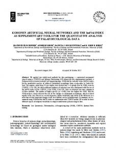
Background Analysis Figure 3 is a MST based on three conventional metrics, molar length (LBL), breadth (LBB) and crown cross-sectional area (LBL × LBB). As expected, the array is mainly influenced by size, as evidenced by its linearity and lack of parallel adjacencies. Specimens having the smallest measurements, the callitrichines, form one stem of the MST opposite those having the largest dimensions, the catarrhines. Within platyrrhines, most lower and upper molars are segregated by size. This has the effect of sorting some species as well. The uppers and lowers of Callicebus and Aotus are not well separated from one another, however. Elsewhere among platyrrhines, the only notable branching structure in the MST is confined to its central section, representing upper molars of Callithrix species, Callimico and Saimiri. The importance of this, like the few small branches evident elsewhere, is moot. Catarrhine molars present no clear upper-lower molar separation because of the near mirror image construction of their bilophodont cheek teeth. This same effect is repeated throughout the analyses. The limited sorting of the catarrhine species that does occur is also an effect of size differences.
Neural Networks and 3-D Digital Morphology
Folia Primatol 2005;76:303–324
311
Fig. 3. MST based on untransformed linear measures. Upper case and lower case for all
figures denote upper and lower molars, respectively. Letter abbreviations for all figures: Platyrrhines – CJ = Callithrix jacchus; CP = Callithrix penicillata; CG = Callimico goeldii; SS = Saimiri sciureus; CM = Callicebus moloch; AT = Aotus trivirgatus; Catarrhines – CS = Colobus satanus; MN = Macaca nigra; PR = ?Prohylobates sp.; OR = Oreopithecus bambolii; PP = Piliocolobus pennantii; PV = Procolobus verus; RA = Rangwapithecus gordoni.
Using 3-D measures describing cusp height, cusp location and occlusal table area as descriptors alters the associative potential of the MST in a few ways, but it does not demonstrably improve the analysis for the entire sample (fig. 4). Overall, there is less linearity and more adjacency in the display because individuals of some species are clustered more tightly, ostensibly because of the richer input information. A size vector continues to dominate the output, but there is also some sorting based on shape and/or taxonomic effects. For example, Callimico uppers are no longer associated with Saimiri (fig. 3), and they form a coherent group linked with Callithrix. In addition, Saimiri, Callicebus and Aotus uppers are tightly 312
Folia Primatol 2005;76:303–324
King/Rosenberger/Kanda
Fig. 4. MST based on untransformed 3-D measures.
associated. Thus, platyrrhines with three- and four-cusped crowns are being discriminated by the 3-D measures. Saimiri lowers are not interposed between uppers and lowers of the callitrichines, as before. Rather, the uppers and lowers of all callitrichines are mapped together. For the catarrhines, the 3-D MST is similar to the display based on linear dimensions, but there is better segregation of 3 taxa, Oreopithecus, ?Prohylobates and Procolobus verus, where uppers and lowers of the same species cluster together. SOM Analysis A SOM based on digital morphology measures (fig. 5) organizes the information differently and, as seen in the MST (fig. 6) based on the SOM, in a more complex fashion. The SOM matrix suggests a strong taxonomic and morphological effect. This is highlighted diagrammatically by the blank cells, which imply strong disjunctions in pattern matching. Thus, a trace of blanks sets off the bottom right quadrant of the SOM, which is occupied entirely by platyrrhine lower molars. An irregular series of blanks separates all catarrhine teeth in the upper right quadrant. Platyrrhines with three-cusped molars tend toward the bottom left, and those with four-cusped teeth tend toward the top left corners of the matrix. Within these four quadrants, there is also some taxonomic structure, as individuals of the same species have a propensity to localize in adjacent cells. Finally, there is some data compression, as expected. For example, only 9 of 10 Saimiri uppers and 8 of 10 Saimiri Neural Networks and 3-D Digital Morphology
Folia Primatol 2005;76:303–324
313
Fig. 5. SOM based on untransformed 3-D measures (see text).
lowers appear in the matrix. The other specimens have been suppressed as redundant cases. Turning to the MST based on the weights of each of the cases that were classified in the SOM (fig. 5) as well as the blanks, the overall complexity of the tree, with numerous well-defined clusters and linkages, is profoundly different from the relatively linear MSTs based on raw data (fig. 3, 4). Groups are strongly partitioned or anchored by the empty cells of the SOM. Several clusters are rooted to the backbone of the MST through blanks. They depict the hierarchy of pattern matching decisions linking each of the individual cases. There are several interesting points of correspondence between this SOM tree and those based on raw measures. First, Aotus and Callicebus, together, continue to occupy adjacent space near the left central core of the MST. This result appears to be driven by resemblance in their upper molars and by mutual resemblances shared with Saimiri (in M2) and the catarrhines (in M2/2) as well. All of these forms have quadrate upper crowns. Second, the lower molars of individual platyrrhine species, although grouping together in a salient partition, are less well resolved taxonomically by the SOM than are their upper molars. The three most coherent clusters defined by the MST (fig. 6) represent callitrichine upper molars, Saimiri uppers and all catarrhine teeth. An offset comprising a unit of Saimiri + Callithrix + Callimico uppers is evident, but this also includes an anomaly, the artificially segmented Saimiri group. This two-tier organization of cebid New World monkeys derived from the SOM data differs in interesting ways from the previous MSTs. In the background study of raw data, caliper measures linked Saimiri uppers and Callimico + Callithrix uppers (fig. 3), presumably because of size. Digital morphology measures associated Saimiri uppers with other four-cusped platyrrhines, Aotus and Callicebus, apparently based on form. The SOM-based MST spatially separates Saimiri uppers from the latter, but places them as a point of linkage to the three-cusped callitrichines. It also places Saimiri lowers well within the callitrichine cluster. 314
Folia Primatol 2005;76:303–324
King/Rosenberger/Kanda
Fig. 6. MST based on SOM weights derived from 3-D measures.
An improved clustering is well illustrated among callitrichines. Uppers of the 5 C. pennicillata individuals are linked intraspecifically in an hierarchy, offset interspecifically through a blank space (implying absence of an existing case match), but clearly associated with the C. jacchus group. Four of 5 C. jacchus are also interlinked. However, there is no clear separation of C. jacchus from Callimico uppers due to the misclassification of the 1 C. jacchus outlier. Were this case removed, it seems likely all Callimico individuals would be identified as a discrete unit. If so, the aggregation of C. jacchus might also resolve. The well-defined Saimiri uppers are also split up, with 2 of 9 individuals appearing as outliers. Among catarrhines, systematic improvements are less evident (fig. 6). There is a tendency to divide colobines from the others, as before (fig. 3, 4), and a few individual cases and taxa are better sorted out. The single Rangwapithecus upper molar and 2 ?Prohylobates lowers, for example, are outliers as expected. One ?Prohylobates tooth is fairly worn while the other is not. Oreopithecus uppers, and Colobus satanus uppers and lowers, also form tighter clusters. Overall, the main benefit here is that catarrhines are strongly demarcated from platyrrhines at the cluster root.
Neural Networks and 3-D Digital Morphology
Folia Primatol 2005;76:303–324
315
Fig. 7. SOM based on 3-D measures, platyrrhines only.
Revising the Data Set In an effort to reduce taxonomic noise specific to our sample (which was constructed in an intentionally lax fashion, but with an eye toward diversity), we examined platyrrhines more closely by eliminating catarrhines from the analysis (i.e. reduced biological variation). A SOM based on the 62 New World monkey cases produced similar results in terms of clusters and within-group links, and a much simpler MST (fig. 7, 8). Several points are of interest. First, the 2-D matrix (fig. 7) sorted most platyrrhines by a tooth axis (horizontally) and a taxonomic axis (vertically), similar to the all-cases SOM: lower teeth on the right and upper teeth on the left of the matrix, with the exception of Aotus and Callicebus. Also, nearly all of the top 40 cells display Callithrix molars, uppers on the left and lowers on the right, strongly divided by a trace of blanks. The bottom 2 rows on the right are exclusively M2s of Aotus and Callicebus. There is a separation of Saimiri M2s in the middle and left lower quadrant of the SOM. Only the Callimico molars appear in cells widely offset diagonally in the SOM, with uppers and lowers falling far apart on the margins of the two Callithrix arrays. In general, the MST (fig. 8) based on this SOM also sorts taxa from left to right, whereas the top and bottom clusters relate to upper and lower molars, respectively. This pattern is repeated in the central section of the backbone, where Aotus and Callicebus are represented. As with all the previous tests, here the uppers tend to give a better definition than the lowers. In addition, as with the SOM based on the full platyrrhine-catarrhine sample, Saimiri and callitrichine uppers are segregated, but linked to one another. Saimiri lowers, and Callicebus and Aotus uppers and lowers, are the connecting elements. Saimiri uppers are also less diffusely organized than in the platyrrhine-catarrhine sample, but the branching structure of the lowers is not easy to interpret. Nevertheless, the Callithrix molars are clustered together here, whereas they were divided into two groups in the larger sample. Another interspecific improvement appears here for the first time: Aotus and Callicebus upper molars are clearly sorted into 2 clusters. 316
Folia Primatol 2005;76:303–324
King/Rosenberger/Kanda
Fig. 8. MST based on SOM weights derived from 3-D measures, platyrrhines only.
SOM Comparison to a Principal-Component Analysis We also conducted a principal-component analysis (PCA) of the 83 virtual specimens as a comparison with a more conventional multivariate analysis approach. PCA exploits the fact that in many cases where the dimension of the input vector is large (12-D in our case) the components of the vectors may be highly correlated (redundant). PCA is often used for its ability to orthogonalize the components of the input vector (so that they are uncorrelated with each other), to order the resulting orthogonal components (principal components) so that those with the largest variation come first and to eliminate those components that contribute the least to the variation in the data set. The first 5 principal components for the full sample of taxa based on 3-D measures are provided in Appendix 2. Figure 9 and the data in Appendix 2 show that size evidently drives PCA 1, as expected when using untransformed measurements. Size was also a strong factor in the SOM, which distributes all the larger taxa in the right upper quadrant, with the smallest taxa in the left lower quadrant. One obvious result for the PCA is that, as a Neural Networks and 3-D Digital Morphology
Folia Primatol 2005;76:303–324
317
Fig. 9. Projection of the first 2 principal components for the full sample of taxa based on
3-D measures.
taxon, Saimiri molars are separated out by PCA 1 and 2. However, the SOM also recognized and distinguished Saimiri uppers and lowers as well, associating them with the equivalent teeth of the other platyrrhines. In addition, the SOM associated Saimiri with the other platyrrhines, rather than differentiating them uniquely from all other samples. Overall, both approaches (SOM and PCA) appear to discriminate platyrrhines from catarrhines. While the taxonomic structure of both approaches is similar, overall the SOM seems superior in consistently discriminating uppers from lowers using the same suite of measurements. Figure 10 shows a projection on the first 2 principal components for only the platyrrhines. This PCA mapping resembles the patterns of segregation of the SOM that were also based on platyrrhine only, with the large and smaller taxa being distinguished and the uppers and lowers of callitrichines also being divided (fig. 7). However, neither the PCA axis alone nor in combination distinguishes Saimiri upper and lower molars from one another, which is a strong feature of the SOM. In addition, the PCA is unable to distinguish the three-cusped uppers of Callimico from the four-cusped molars of Aotus and Callicebus. That, too, is a prominent feature of the SOM, which aligns Callimico uppers with those of the much smaller, but similarly shaped uppers of Callithrix and Cebuella. 318
Folia Primatol 2005;76:303–324
King/Rosenberger/Kanda
Fig. 10. Projection on the first 2 principal components, platyrrhines only.
In general, the SOM analysis was validated by the PCA approach. However, the SOM provided additional insight into the data set beyond what could be seen with PCA alone. This is because the SOM retains more of the higher dimensionality information from the data set in its 2-D mapping of the taxa. Discussion
Using simple Euclidean distances and MSTs as yardsticks, we have shown that an ANN using 3-D digital morphology measures extracts more systematic information from molar form than untransformed caliper (linear) measures or digital morphology (shape) measures. In spite of a very heterogeneous sample, a self-organized ANN is able to sort upper and lower molars, and phenetically segregate taxa at several levels of the Linnean hierarchy. With this approach, 8 measures that capture topographic as well as size information about upper and lower second molars were sufficient to successively cluster unidentified individuals into natural groups – species, possible sister-species (or subspecies), tribes and subfamilies, and even higher levels (catarrhines vs. platyrrhines). Balances between strong morphological disjunctions and phylogenetic continuity were also maintained. For example, the three-cusped callitrichines were grouped apart from four-cusped Saimiri, yet both were isolated (as cebids) on a separate branch relative to the more distantly related Aotus and Callicebus (atelids). To our knowledge, there is no comparable high-dimensional biometric study of primate molars that demonstrates similar phenetic results. Nevertheless, these are not entirely unexpected. Most of the morphological clusters identified by the SOM are, in fact, identifiable using eyeball inspection, with one notable exception. Neural Networks and 3-D Digital Morphology
Folia Primatol 2005;76:303–324
319
The association of Aotus and Callicebus was not anticipated. Visual study would not necessarily stress their gross resemblance, certainly not in the upper molar form. No active worker has claimed that the molars of these two genera are as similar as the SOM implies, although many have remarked on resemblances in their skeletons and in cranial morphology. There is also significant controversy over the phylogenetic relationships of these animals [Schneider and Rosenberger, 1997]. The discovery of embedded occlusal resemblances is thus an unexpected vote of phenetic support for the idea that Aotus and Callicebus are closely related and that similarities between Aotus and Callimico lower molars are, in fact, convergent [Rosenberger et al., 1990]. Misclassifications were produced in this study, but they do not necessarily point to weaknesses in the methodology. There appear to be 3 possible components affecting errors. First is information content. Upper molars may yield more or richer information than lowers. In most of our runs, lowers tended to cluster more diffusely and were more likely than uppers to annex individuals that are not conspecifics. The reduced, platyrrhine-only data set also corroborates the notion of a differential in information richness. Upper molar clusters for 3 cebid genera included 40% blanks in the MST. Lower clusters contained 58% blanks. More ‘force fits’ occurred with lower teeth. A second source of error is sample composition. Our subgroups were of uneven sample sizes and composition. They included both closely and distantly related lineages, and the catarrhines have a fundamentally different gestalt than the platyrrhines. Catarrhines are large in size, present a more continuous morphocline of shapes, are morphologically uniform across species and have relatively isomorphic, mirror image molars. Removing catarrhines improved the clustering efficiency for various platyrrhine groups. This amplifies the importance of selecting an appropriate study group when framing a systematic question. A third factor is variability. In attempting to pattern-match individual cases, we skirt the issue of population variation. Several individual outliers, notably 1 or 2 specimens of Saimiri, Aotus and Callimico, differ by very small units of measure, fractions of a millimeter or square millimeter. Given the very favorable results of the ANN overall, our working hypothesis is that a number of these individuals were set off because our data set inadequately represents the population of shape patterns for the species. In our view, the interaction of these risks had little influence on a robust, net result. No gross misclassifications occurred. For example, in the reduced data set, of the 15 upper callitrichine molars only 1, a C. jacchus, was annexed in error, to a Callimico, which was also an outlier. Our supposition is that more individuals and more sophisticated 3-D measures that enhance the capture of morphology will reduce the error margin still further. Acknowledgements
We thank the Department of Conservation Biology, National Zoological Park, Smithsonian Institution, for logistical support. Support from the National Science Foundation, LSB Leakey Foundation, Wenner Gren Foundation and the National Institute for Standards and Technology contributed to this project. We dedicate this paper to the late Charles Calvo, a man of shining brilliance and boundless good will.
320
Folia Primatol 2005;76:303–324
King/Rosenberger/Kanda
Appendix 1
Final input weight values after training used to calculate the SOM for the full sample of taxa based on 3-D measures. The columns represent the measurements, and the 100 rows represent the cells (neurons) of the 10 × 10 matrix. 1 2 3 4 5 6 7 8 9 10 11 12 13 14 15 16 17 18 19 20 21 22 23 24 25 26 27 28 29 30 31 32 33 34 35 36 37 38 39 40 41 42 43 44 45 46 47 48 49 50 51 52
0.0578 0.0455 0.0415 0.0186 0.0061 0.0051 0.0052 0.0035 0.0101 0.0017 0.0506 0.0510 0.0454 0.0297 0.0066 0.0163 0.0123 0.0157 0.0285 0.0086 0.0505 0.0547 0.0657 0.0430 0.0217 0.0203 0.0251 0.0288 0.0254 0.0233 0.0347 0.0491 0.0628 0.0513 0.0461 0.0439 0.0326 0.0358 0.0326 0.0439 0.0545 0.0538 0.0301 0.0000 0.0328 0.0490 0.0437 0.0376 0.0387 0.0417 0.0282 0.0184
0.0882 0.0938 0.1279 0.0609 0.0250 0.0282 0.0281 0.0245 0.0311 0.0220 0.1138 0.1166 0.1329 0.0730 0.0271 0.0294 0.0508 0.0327 0.0459 0.0511 0.1123 0.1236 0.1447 0.0968 0.0406 0.0350 0.0540 0.0556 0.0526 0.0530 0.1435 0.1434 0.1468 0.1141 0.0589 0.0726 0.0622 0.0655 0.0662 0.0872 0.1521 0.1414 0.0763 0.0000 0.0576 0.1044 0.0866 0.0773 0.0794 0.0806 0.0773 0.0497
0.0748 0.0549 0.0493 0.0232 0.0062 0.0092 0.0108 0.0106 0.0136 0.0033 0.0762 0.0758 0.0796 0.0411 0.0069 0.0194 0.0165 0.0203 0.0305 0.0099 0.0879 0.0896 0.1071 0.0635 0.0174 0.0185 0.0284 0.0321 0.0261 0.0302 0.0617 0.0650 0.1062 0.0783 0.0325 0.0377 0.0401 0.0396 0.0358 0.0437 0.0781 0.0828 0.0871 0.1046 0.0695 0.0517 0.0479 0.0431 0.0503 0.0558 0.0886 0.0804
0.1010 0.0867 0.0982 0.0502 0.0245 0.0258 0.0307 0.0314 0.0369 0.0295 0.1022 0.1045 0.1075 0.0644 0.0281 0.0391 0.0413 0.0402 0.0510 0.0625 0.1050 0.1110 0.1337 0.0900 0.0408 0.0329 0.0504 0.0549 0.0476 0.0726 0.0941 0.1331 0.1367 0.1060 0.0447 0.0621 0.0603 0.0650 0.0671 0.0710 0.1171 0.1101 0.1244 0.1207 0.1051 0.0957 0.0878 0.0871 0.1155 0.1222 0.1156 0.1146
0.0396 0.0620 0.0567 0.0290 0.0111 0.0072 0.0125 0.0134 0.0197 0.0107 0.0831 0.0799 0.0907 0.0431 0.0091 0.0177 0.0137 0.0305 0.0298 0.0402 0.0855 0.1023 0.0899 0.0579 0.0177 0.0218 0.0331 0.0438 0.0470 0.0477 0.0841 0.0943 0.1127 0.0777 0.0334 0.0392 0.0499 0.0584 0.0526 0.0508 0.0813 0.0900 0.0959 0.0966 0.0687 0.0533 0.0569 0.0669 0.0721 0.0667 0.0845 0.0840
Neural Networks and 3-D Digital Morphology
0.0955 0.0955 0.0801 0.0503 0.0328 0.0348 0.0302 0.0299 0.0354 0.0280 0.1169 0.1147 0.1218 0.0652 0.0315 0.0333 0.0266 0.0450 0.0445 0.0536 0.1416 0.1347 0.1283 0.0843 0.0332 0.0348 0.0453 0.0556 0.0616 0.0558 0.1219 0.1324 0.1422 0.1052 0.0560 0.0652 0.0579 0.0674 0.0641 0.0660 0.1268 0.1125 0.1320 0.1357 0.1041 0.0914 0.0834 0.0881 0.1040 0.1022 0.1305 0.1288
0.0347 0.0576 0.0467 0.0206 0.0056 0.0026 0.0039 0.0020 0.0113 0.0030 0.0476 0.0513 0.0549 0.0285 0.0037 0.0165 0.0104 0.0205 0.0279 0.0259 0.0440 0.0487 0.0461 0.0351 0.0195 0.0190 0.0285 0.0370 0.0369 0.0314 0.0540 0.0666 0.0610 0.0457 0.0408 0.0442 0.0406 0.0510 0.0418 0.0404 0.0472 0.0603 0.0796 0.0908 0.0666 0.0577 0.0523 0.0551 0.0492 0.0390 0.0774 0.0879
0.0779 0.0889 0.0804 0.0405 0.0244 0.0260 0.0276 0.0308 0.0334 0.0304 0.0880 0.0877 0.0860 0.0481 0.0155 0.0245 0.0205 0.0299 0.0389 0.0360 0.0765 0.0971 0.0845 0.0593 0.0289 0.0292 0.0396 0.0483 0.0504 0.0597 0.0933 0.0824 0.0924 0.0722 0.0599 0.0653 0.0516 0.0622 0.0591 0.0591 0.0935 0.1028 0.1220 0.1426 0.1051 0.0870 0.0759 0.0766 0.0735 0.0650 0.1356 0.1423
Folia Primatol 2005;76:303–324
0.1898 0.1849 0.1804 0.1190 0.0825 0.0816 0.0850 0.0887 0.0904 0.0861 0.1921 0.1916 0.1990 0.1302 0.0894 0.0887 0.0770 0.0953 0.0931 0.1001 0.2035 0.1979 0.1861 0.1486 0.1014 0.0908 0.1159 0.1275 0.1086 0.1183 0.1928 0.1981 0.2078 0.1716 0.1312 0.1462 0.1469 0.1706 0.1394 0.1218 0.2138 0.2008 0.2278 0.2587 0.2076 0.1833 0.1814 0.1958 0.2050 0.1860 0.2298 0.2397
0.2415 0.2283 0.2350 0.1417 0.0730 0.0839 0.0764 0.0725 0.0807 0.0660 0.2770 0.2750 0.2985 0.1760 0.0900 0.0911 0.0864 0.0861 0.1064 0.1049 0.3052 0.3130 0.3066 0.2200 0.1175 0.1084 0.1051 0.1072 0.1017 0.1229 0.3108 0.3051 0.3260 0.2559 0.1209 0.1520 0.1255 0.1130 0.1173 0.1197 0.3000 0.3133 0.3240 0.3346 0.2486 0.2170 0.1805 0.1623 0.1699 0.1617 0.3306 0.3238
0.7538 0.7693 0.7766 0.8031 0.8032 0.7862 0.7586 0.7420 0.6995 0.6523 0.7698 0.7619 0.7466 0.8012 0.8085 0.7972 0.7561 0.7104 0.7054 0.6817 0.7634 0.7646 0.7297 0.7943 0.8452 0.8130 0.7589 0.7151 0.6865 0.6302 0.7774 0.7632 0.7332 0.7786 0.8161 0.7931 0.7683 0.7064 0.6673 0.6142 0.7887 0.7833 0.7582 0.7531 0.7651 0.7316 0.7400 0.7159 0.6803 0.6509 0.7790 0.7726
321
0.5409 0.5257 0.5107 0.5552 0.5827 0.6039 0.6385 0.6578 0.7004 0.7481 0.4811 0.4944 0.4927 0.5375 0.5721 0.5857 0.6394 0.6865 0.6862 0.7079 0.4623 0.4462 0.5005 0.5099 0.5048 0.5596 0.6223 0.6666 0.7002 0.7445 0.4404 0.4501 0.4608 0.4913 0.5329 0.5497 0.5933 0.6583 0.7059 0.7517 0.4033 0.4137 0.4367 0.4150 0.5083 0.5804 0.5906 0.6204 0.6472 0.6846 0.3931 0.4085
Appendix 1 ( continued ) 53 54 55 56 57 58 59 60 61 62 63 64 65 66 67 68 69 70 71 72 73 74 75 76 77 78 79 80 81 82 83 84 85 86 87 88 89 90 91 92 93 94 95 96 97 98 99 100
0.0000 0.0000 0.0177 0.0667 0.0594 0.0376 0.0313 0.0470 0.0000 0.0000 0.0000 0.0000 0.0505 0.0752 0.0698 0.0706 0.0659 0.0354 0.0000 0.0000 0.0000 0.0356 0.0737 0.0888 0.0731 0.0641 0.0641 0.0567 0.0000 0.0000 0.0000 0.0445 0.0818 0.1039 0.0698 0.0813 0.0709 0.0579 0.0000 0.0000 0.0000 0.0289 0.0816 0.0918 0.0914 0.0939 0.1031 0.0793
322
0.0000 0.0000 0.0317 0.1153 0.1047 0.0844 0.0765 0.0842 0.0000 0.0000 0.0000 0.0000 0.0774 0.1130 0.1080 0.1148 0.1113 0.0720 0.0000 0.0000 0.0000 0.0554 0.1119 0.1188 0.1012 0.1125 0.1040 0.1068 0.0000 0.0000 0.0000 0.0702 0.1304 0.1305 0.1423 0.1265 0.1253 0.0906 0.0000 0.0000 0.0000 0.0502 0.1449 0.1493 0.1244 0.1510 0.1227 0.1265
0.0698 0.0915 0.0903 0.0820 0.0746 0.0428 0.0494 0.0737 0.0993 0.0789 0.0737 0.0830 0.1083 0.1039 0.0959 0.0866 0.0819 0.0592 0.0795 0.0699 0.0476 0.0884 0.1105 0.1214 0.1097 0.1088 0.0913 0.1050 0.0726 0.0874 0.0831 0.1009 0.1291 0.1299 0.1144 0.1084 0.1030 0.0917 0.0901 0.0894 0.0751 0.1000 0.1393 0.1315 0.1259 0.1235 0.1119 0.0916
0.1166 0.1137 0.1284 0.1721 0.1304 0.1035 0.1475 0.1536 0.1157 0.1077 0.1114 0.1196 0.1602 0.1648 0.1304 0.1289 0.1478 0.1397 0.0997 0.1082 0.1006 0.1421 0.1801 0.1880 0.1828 0.1552 0.1530 0.1570 0.1177 0.1248 0.1216 0.1620 0.1854 0.2090 0.1911 0.1603 0.1633 0.1518 0.1255 0.1373 0.1311 0.1600 0.2251 0.2095 0.1770 0.1490 0.1600 0.1567
0.0796 0.0905 0.0884 0.0757 0.0859 0.0811 0.0831 0.0840 0.0841 0.0853 0.0945 0.0928 0.1072 0.1047 0.1136 0.1007 0.0668 0.1006 0.0795 0.1070 0.1049 0.1126 0.1092 0.0992 0.1195 0.1088 0.0957 0.1189 0.1094 0.1200 0.1453 0.1279 0.1355 0.1165 0.1395 0.1163 0.1236 0.1441 0.1296 0.1129 0.1329 0.1394 0.1350 0.1041 0.1322 0.1296 0.1119 0.1161
0.1264 0.1352 0.1290 0.1208 0.1237 0.1094 0.1307 0.1262 0.1367 0.1439 0.1429 0.1684 0.1597 0.1526 0.1564 0.1449 0.0944 0.1500 0.1310 0.1307 0.1535 0.1661 0.1787 0.1540 0.1621 0.1394 0.1353 0.1560 0.1653 0.1651 0.1663 0.1720 0.1803 0.1666 0.1898 0.1513 0.1597 0.1802 0.1640 0.1535 0.1682 0.1758 0.1885 0.1671 0.1649 0.1541 0.1542 0.1416
Folia Primatol 2005;76:303–324
0.1025 0.0969 0.0816 0.0487 0.0564 0.0626 0.0494 0.0414 0.1040 0.1130 0.0942 0.0830 0.0672 0.0505 0.0521 0.0536 0.0668 0.0616 0.0862 0.0834 0.0941 0.0759 0.0382 0.0431 0.0585 0.0465 0.0519 0.0548 0.0940 0.0874 0.0761 0.0699 0.0716 0.0551 0.0530 0.0474 0.0704 0.0612 0.0618 0.0840 0.0660 0.0703 0.0675 0.0479 0.0618 0.0418 0.0638 0.0850
0.1591 0.1570 0.1323 0.0856 0.0975 0.0956 0.0650 0.0731 0.1776 0.1620 0.1473 0.1233 0.1189 0.0964 0.1034 0.1120 0.1113 0.1037 0.1501 0.1487 0.1406 0.1284 0.1010 0.0809 0.1085 0.0995 0.0838 0.0994 0.1308 0.1363 0.1146 0.1171 0.1240 0.1007 0.0921 0.1084 0.1037 0.1147 0.1124 0.1020 0.1058 0.1089 0.1027 0.0740 0.1072 0.1092 0.1041 0.1048
0.2594 0.2435 0.2442 0.2478 0.2375 0.2307 0.2258 0.2152 0.2477 0.2537 0.2542 0.2588 0.2782 0.2776 0.2449 0.2475 0.2672 0.2055 0.2654 0.2535 0.2562 0.2732 0.2906 0.3264 0.3047 0.2426 0.2473 0.2433 0.2533 0.2285 0.2188 0.2646 0.2876 0.2933 0.2958 0.2687 0.2452 0.2588 0.2146 0.2113 0.2143 0.2425 0.2813 0.2903 0.2810 0.2673 0.2572 0.2483
0.3183 0.3386 0.3152 0.2568 0.2366 0.2024 0.1813 0.1880 0.3588 0.3251 0.3325 0.3503 0.3081 0.2639 0.2588 0.2503 0.2191 0.1952 0.3360 0.3414 0.3244 0.3196 0.3084 0.2598 0.2584 0.2510 0.2340 0.2443 0.3627 0.3274 0.3080 0.3079 0.2902 0.2686 0.2860 0.2631 0.2514 0.2610 0.3746 0.3368 0.3174 0.3092 0.2996 0.2808 0.2770 0.2357 0.2366 0.2416
King/Rosenberger/Kanda
0.7565 0.7616 0.7496 0.7065 0.6967 0.7086 0.6799 0.6580 0.7607 0.7738 0.7608 0.7421 0.6991 0.6726 0.6806 0.6586 0.6572 0.6574 0.7963 0.7684 0.7687 0.7195 0.6563 0.6501 0.6460 0.6553 0.6593 0.6399 0.7731 0.7796 0.7700 0.7011 0.6533 0.6220 0.6069 0.6267 0.6288 0.6180 0.7937 0.7884 0.7524 0.7140 0.5992 0.5957 0.6079 0.6173 0.6195 0.6353
0.4273 0.4053 0.4522 0.5380 0.5743 0.5926 0.6263 0.6458 0.3739 0.3826 0.4103 0.4235 0.4873 0.5463 0.5624 0.5946 0.6109 0.6410 0.3360 0.3932 0.4033 0.4591 0.5212 0.5379 0.5534 0.5939 0.6046 0.6083 0.3497 0.3764 0.4183 0.4857 0.5101 0.5587 0.5665 0.5962 0.6056 0.6082 0.3158 0.3739 0.4504 0.4793 0.5528 0.5862 0.5863 0.6071 0.6156 0.6079
Appendix 2
First 5 principal components Taxon
Colobus satanus Piliocolobus pennantii Procolobus verus Macaca nigra Oreopithecus bambolii Oreopithecus bambolii Oreopithecus bambolii ?Prohylobates sp. ?Prohylobates sp. Aotus trivirgatus Aotus trivirgatus Callicebus moloch Callicebus moloch Callicebus moloch Saimiri sciureus Saimiri sciureus Saimiri sciureus Saimiri sciureus Saimiri sciureus Saimiri sciureus Saimiri sciureus Saimiri sciureus Saimiri sciureus Saimiri sciureus Callithrix jacchus Callithrix jacchus Callithrix jacchus Callithrix jacchus Callithrix jacchus Callithrix jacchus Callithrix penicillata Callithrix penicillata Callithrix penicillata Callithrix penicillata Callithrix penicillata Callimico goeldii Callimico goeldii Callimico goeldii Callimico goeldii Callimico goeldii Colobus satanus Piliocolobus pennantii Piliocolobus pennantii Procolobus verus Macaca nigra Oreopithecus bambolii Oreopithecus bambolii Oreopithecus bambolii Rangwapithecus gordoni ?Prohylobates sp. ?Prohylobates sp. ?Prohylobates sp. Aotus trivirgatus Aotus trivirgatus Callicebus moloch Callicebus moloch
Principal components first
second
third
fourth
fifth
–5.2774 –2.1689 –3.5584 –6.3772 –5.4294 –5.8431 –6.385 –4.0486 –5.2238 –0.8959 –0.2833 –0.0042 –0.1205 –0.2126 –1.5242 –1.512 –1.2992 –1.4126 –1.4614 –1.3143 –1.3962 –1.542 –1.5216 –1.548 –2.3759 –2.1834 –2.3173 –2.028 –2.2425 –2.3062 –2.0412 –2.0805 –2.1951 –2.3901 –1.805 –1.5897 –1.3949 –1.9834 –1.8396 –1.6559 –5.5016 –4.5616 –2.4035 –2.708 –6.071 –7.1915 –4.3251 –5.9303 –7.2392 –4.6391 –3.8077 –3.6644 –0.6623 –0.1881 –0.2183 –0.3957
–3.6079 –3.4306 –3.5106 –2.5476 –5.6986 –3.2692 –5.2281 –3.4537 –2.1861 –0.1261 –0.1991 –0.857 –0.2461 –0.1193 –0.2697 –0.3894 –0.5344 –0.4853 –1.5546 –0.4367 –0.9843 –0.4164 –0.9642 –0.0804 –0.2994 –0.2708 –0.2807 –0.1868 –1.1772 –0.1361 –0.4732 –0.0461 –1.1035 –0.2135 –0.4853 –0.0591 –1.2822 –0.0179 –0.205 –0.7847 –3.7211 –0.2895 –3.4328 –1.4097 –1.5395 –3.8978 –4.4818 –4.9528 –0.0737 –1.6385 –0.0401 –1.089 –0.6457 –0.1197 –0.3719 –0.4801
–1.8625 –1.2569 –0.1235 –1.592 –0.1559 –1.0344 –0.3493 –0.6735 –0.6242 –0.5055 –0.4287 –0.2896 –1.0936 –0.534 –0.933 –0.9997 –0.7819 –0.5238 –0.0243 –1.1475 –0.0144 –1.0562 –0.5328 –1.0859 –0.6138 –0.7195 –1.8797 –2.0881 –1.8081 –1.3491 –0.8726 –1.216 –1.3599 –1.0777 –1.5253 –0.837 –1.573 –1.3438 –0.5267 –1.4735 –0.0497 –2.8031 –0.8597 –0.8319 –0.2859 –0.1992 –1.1773 –1.3083 –0.7445 –0.1207 –0.3255 –0.745 –2.2034 –0.2669 –0.3324 –0.08
–0.1477 –0.3622 –0.384 –0.3299 –1.287 –0.6419 –0.333 –1.7509 –0.3787 –1.5061 –1.3072 –0.9981 –0.8051 –1.8813 –0.2822 –0.0024 –0.683 –0.1975 –0.9895 –0.8006 –0.7797 –0.1306 –0.316 –0.0484 –0.7305 –0.4975 –0.2305 –0.4205 –0.2802 –0.2166 –0.1471 –0.7479 –0.2531 –0.4948 –0.6175 –0.5022 –0.1508 –0.2674 –0.9843 –0.4206 –1.1112 –3.1029 –0.2409 –1.2257 –0.9597 –0.029 –0.2303 –1.2911 –0.6167 –0.815 –0.0371 –0.523 –1.5759 –0.0097 –0.1503 –0.2503
–0.6161 –0.2271 –0.4589 –0.2262 –0.3653 –1.0739 –2.7072 –0.8433 –0.9205 –0.6467 –0.0758 –0.2911 –0.3274 –1.2293 –0.2505 –1.0416 –0.5915 –0.7053 –0.5219 –0.798 –0.3387 –0.736 –0.4234 –0.3415 –0.0907 –0.2641 –0.2712 –0.0638 –0.1317 –0.7956 –0.3349 –0.1769 –0.5347 –0.5159 –0.01 –0.5978 –0.0928 –0.855 –0.7384 –1.9047 –0.1532 –0.2827 –0.4679 –1.1719 –0.8662 –0.1317 –1.1376 –0.1786 –0.4268 –0.5127 –1.8055 –1.7411 –0.8553 –1.3224 –0.6726 –0.6628
Neural Networks and 3-D Digital Morphology
Folia Primatol 2005;76:303–324
323
Appendix 2 (continued) Taxon
Principal components
Callicebus moloch Saimiri sciureus Saimiri sciureus Saimiri sciureus Saimiri sciureus Saimiri sciureus Saimiri sciureus Saimiri sciureus Saimiri sciureus Saimiri sciureus Saimiri sciureus Callithrix jacchus Callithrix jacchus Callithrix jacchus Callithrix jacchus Callithrix jacchus Callithrix jacchus Callithrix penicillata Callithrix penicillata Callithrix penicillata Callithrix penicillata Callithrix penicillata Callimico goeldii Callimico goeldii Callimico goeldii Callimico goeldii Callimico goeldii Callithrix penicillata Callithrix penicillata Callithrix penicillata Callimico goeldii Callimico goeldii Callimico goeldii Callimico goeldii Callimico goeldii
first
second
third
fourth
fifth
–0.484 –1.2038 –1.068 –1.4585 –1.3919 –1.6101 –1.3985 –1.5607 –1.0044 –1.5508 –1.4007 –2.4526 –2.3872 –2.7313 –2.5738 –2.6635 –2.7948 –2.3906 –2.796 –2.6957 –2.5943 –2.8837 –1.8209 –1.9634 –1.9676 –2.3104 –1.8233 –2.6957 –2.5943 –2.8837 –1.8209 –1.9634 –1.9676 –2.3104 –1.8233
–0.6234 –0.5018 –0.3774 –0.5589 –0.2924 –0.9832 –0.5291 –0.0504 –0.7461 –0.3543 –0.5836 –1.5341 –1.616 –1.6614 –0.7792 –1.2238 –1.19 –1.0934 –1.5835 –1.1721 –1.1789 –0.7005 –0.0937 –0.0202 –0.5689 –0.8244 –0.7067 –1.1721 –1.1789 –0.7005 –0.0937 –0.0202 –0.5689 –0.8244 –0.7067
–0.2282 –0.599 –0.6352 –0.0136 –0.5555 –0.1244 –0.3477 –0.7139 –0.8598 –0.1382 –0.3206 –1.6705 –1.9983 –1.3092 –1.72 –1.828 –1.7274 –1.854 –1.2694 –1.3984 –1.4705 –1.5207 –2.4427 –2.317 –2.0132 –1.6189 –2.0453 –1.3984 –1.4705 –1.5207 –2.4427 –2.317 –2.0132 –1.6189 –2.0453
–0.7461 –0.4068 –0.9597 –0.4244 –0.5448 –0.4274 –0.1821 –1.2258 –1.0371 –0.3897 –0.9232 –0.3688 –0.6994 –0.8148 –1.1821 –0.1125 –0.0213 –1.1335 –1.3975 –1.8117 –1.5087 –1.498 –0.1503 –0.1893 –0.5179 –0.371 –0.5197 –1.8117 –1.5087 –1.498 –0.1503 –0.1893 –0.5179 –0.371 –0.5197
–0.3438 –0.0002 –1.1686 –0.5111 –0.3604 –0.4596 –0.0799 –0.0388 –0.553 –0.19 –1.6375 –0.8667 –0.871 –0.9849 –0.2577 –0.8042 –0.5229 –0.9404 –0.2533 –0.1367 –0.3286 –0.2228 –1.1611 –0.3802 –0.3261 –1.0229 –0.6185 –0.1367 –0.3286 –0.2228 –1.1611 –0.3802 –0.3261 –1.0229 –0.6185
References King RL (1998). Artificial neural networks and computational intelligence. IEEE Computer Applications in Power 11: 14–25. King RL, Hicks MA, Singer SP (1993). Using unsupervised learning for feature detection in a coal mine roof. Engineering Applications of Artificial Intelligence 6: 565–573. Kohonen T (1989). Self-Organization and Associative Memory. New York, Springer. Kohonen T, Hynninen J, Kangas J, Laaksonen J (1996). SOM-PAK: The Self-Organizing Map Program Package, Report A31. Helsinki, Helsinki University of Technology, Laboratory of Computer and Information Science. Moon TK, Stirling WC (2000). Mathematical Models and Algorithms for Signal Processing. New Jersey, Prentice-Hall. Papadimitriou CH, Steiglitz K (1982). Combinatorial Optimization: Algorithms and Complexity. New Jersey, Prentice-Hall. Rosenberger AL, Setoguchi T, Shigehara N (1990). The fossil record of callitrichine primates. Journal of Human Evolution 19: 209–236. Sammon JW Jr. (1969). A nonlinear mapping for data structure analysis. IEEE Transactions on Computers 18: 401–409. Schneider H, Rosenberger AL (1997). Molecules, morphology and platyrrhine systematics. In Adaptive Radiations of Neotropical Primates (Norconk MA, Rosenberger AL, Garber PA, eds.), pp 3–19. New York, Plenum Press. Stuttgart Neural Network Simulator (SNNS) Version 4.2 (1998). Stuttgart, University of Stuttgart. Ungar PS, M’Kirera F (2003). A solution to the worn tooth conundrum in primate functional anatomy. Proceedings of the National Academy of Sciences USA 100: 3874–3877.
324
Folia Primatol 2005;76:303–324
King/Rosenberger/Kanda